Numerical Simulation of a Self-Similar Cascade of Filament Instabilities
in the Surface Quasigeostrophic System
R. K. Scott* and D. G. Dritschel
School of Mathematics and Statistics, University of St Andrews, St Andrews KY16 9SS, United Kingdom
(Received 12 June 2013; published 11 April 2014)
We provide numerical evidence for the existence of a cascade of filament instabilities in the surface quasigeostrophic system for rotating, stratified flow near a horizontal boundary. The cascade involves geometrically shrinking spatial and temporal scales and implies the singular collapse of the filament width to zero in a finite time. The numerical method is both spatially and temporally adaptive, permitting the accurate simulation of the evolution over an unprecedented range of spatial scales spanning over ten orders of magnitude. It provides the first convincing demonstration of the cascade, in which the large separation of scales between subsequent instabilities has made previous numerical simulation difficult.
DOI:10.1103/PhysRevLett.112.144505 PACS numbers: 47.11.-j, 47.20.Cq,
47.32.C-The surface quasigeostrophic system is a two-dimensional active scalar equation developed as a model for the slow, large-scale motions of rotating, stratified flows of planetary atmospheres and oceans near a horizontal surface or strong jump in stratification such as the midlatitude tropopause [1–3]. It may be expressed by the material advection of a surface temperature fieldθðx; y; tÞby a flow to which it is diagnostically related:
∂θ
∂tþJðψ;θÞ ¼0; θ¼−ð−ΔÞ1=2ψ; (1) whereψ is the stream function, Δis the two-dimensional Laplacian, and Jð·;·Þ is the Jacobean determinant [4]. It differs from the usual two-dimensional Euler equations of incompressible fluid motion through the relation between θ and ψ, where the more local relation in the surface quasigeostrophic case gives rise to more energetic small-scale motions. In fact, the advection term in Eq.(1) possesses a quadratic degree of nonlinearity similar to that of the three-dimensional Euler equations, for vorticity in the case of the Euler equations and for the skew gradient of temperature in the case of the surface quasigeostrophic equations[5–7]; see, in particular, Eq. (13) of Ref.[6]. The similarities between Eq. (1) and the three-dimensional Euler equations have stimulated much research into the regularity of the surface quasigeostrophic system, in particular, whether a singularity in the temperature gradient ∇θmay form in finite time from smooth initial conditions, or whether weak solutions may possess a finite dissipation anomaly in the inviscid limit, the counterpart to the famous Onsager conjecture for turbulent flow governed by the three-dimensional Euler equations[8,9]. Despite the reduced dimensionality, however, the presence of singularities in the surface quasigeostrophic system remains an open problem. When the initial distribution ofθis smooth, it is known that a singularity may not form in finite time if the geometry of the temperature field takes the form of a closing saddle,
involving the growth of unbounded gradients ofθalong a line [10]. Numerical studies of the closing saddle [9,11] indicate double exponential growth∇θ∝exp expt, or an even less rapid evolution with time. Singularities may yet form at isolated points. One scenario for this has been proposed involving a cascade of repeated filament insta-bilities of geometrically shrinking scale[4,12,13]. Because filament growth rates scale with the inverse filament width, were such a cascade of instabilities to follow a self-similar pattern, then a singularity involving the blowup of ∇θ would occur in finite time. However, a large-scale separation between subsequent instabilities (see below) means that such a cascade has been extremely difficult to demonstrate numerically, the most recent results being limited to at best two or three consecutive instabilities before the limits of numerical resolution are reached[14]. Furthermore, uncer-tainties remain over the role of the numerical grid in the triggering of each instability.
In the special case where the temperature distribution comprises a discrete patch (uniform inside a closed contour, zero outside, for example), the relation betweenθ andψ may be expressed in terms of a single contour integral around the patch boundary, in a manner directly analogous to the Biot-Savart law relating electric current to magnetic field. Representing the patch boundary by a closed contour
C, its evolution is then governed by
dxi dt ¼
θ0
2π
Z
C dx0 jxi−x0j
(2)
of a discontinuity in the patch boundary, either through the development of a corner with infinite curvature at a point, or the approach to zero of the minimum distance between two contour segments. In contrast to the smooth case examined in Ref.[14], the filament cross section formed by instabilities of the patch is guaranteed to retain the same trivial profile throughout the evolution. Further, the reduc-tion of the dynamics in the patch case to the evolureduc-tion of a single contour enables the application of a highly efficient Lagrangian contour dynamical algorithm that is here able to capture the patch evolution through a series of instabilities spanning a range of spatial scales on the order of 1010. The cascade is shown to be self-similar upon a uniform rescaling of the independent variables.
For completeness, we note that another potential route to singularity for the patch was identified in numerical experiments of Ref. [16], involving the formation of a corner. While mathematically singular, it is important to recognize that this type of singularity has no counterpart in the evolution of the continuous θ distribution of most relevance to fluid motion: a continuous distribution may develop a corner in a level set of θ without any accom-panying blowup of the temperature gradient. One reason that the instability cascade is important is that the counter-part in the evolution of the continuous distribution may also exist (see below). The extension of the present result to the more general case of the continuous distribution will be addressed in future work.
We solve the evolution of the patch using the contour dynamics method of Dritschel[17], representing the patch boundary by a series of points along a contour that are redistributed according to the boundary shape. The method has been refined here in that the integral [Eq.(2)] aroundC is now computed along a series of global splines connecting the points, ensuring continuity of curvature and the tangent vector at each point. The point distribution along C is determined adaptively according to the curvature ofC, the local value of the strain field, and the minimum separation between adjacent segments of the boundary, more points being added to maintain accuracy as the complexity of the boundary increases. This ensures that accuracy is maintained even in regions of very high curvature and where filaments become narrow.
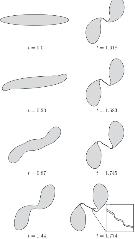
To illustrate the cascade, we consider a patch ofθdefined by an initial elliptical boundary of aspect ratioa¼0.16, as shown in the upper left panel of Fig.1, withθ¼2πinside the boundary and θ¼0 outside. As time increases, the ellipse rotates and deforms, with the tips developing into two distinct lobes separated by a filament (t¼1.44) that subsequently lengthens and thins (t¼1.618tot¼1.745). By t¼1.774, an instability of the central filament has occurred with the development of a series of new lobes connected by new filaments at a much smaller scale (inset). These filaments subsequently become unstable and roll up in a self-similar manner on a shrinking time scale (an
animation of the patch evolution is available in the Supplemental Material [18]).
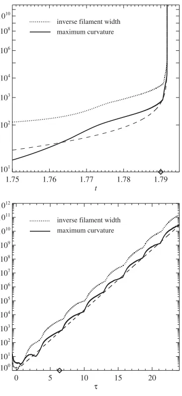
[image:2.612.324.553.55.459.2]The rapid collapse of both time and length scales can be seen by considering the growth of curvatureκand inverse minimum cross-filament widthd−1in time. The develop-ment of the filadevelop-ment instability between t¼1.745 and t¼1.774 involves the accelerating growth in bothκ and d−1; see Fig.2(a). At aroundt¼1.774, this growth slows as the new filament is more gradually extended. Fast growth begins again at around t¼1.791 with the onset of the next filament instability; the shrinking time scales suggest unbounded growth in bothκandd−1at a finite time ts, which is here estimated as ts¼1.791 713 423 533 39; bothκ andd−1 follow approximately1=ðts−tÞ, although with alternating periods of more or less rapid growth
FIG. 1. Snapshots of the patch boundary at selected times prior to the onset of the first filament instability;θ¼2π inside the patch boundary and θ¼0 outside. The final frame shows an
according to whether the smallest filament is in a roll-up or extending phase.
The evolution as the singularity is approached is clarified by introducing a rescaled time variable[16]τ¼−logðts−tÞ. The repeated stages of rapid growth (instability development) followed by a saturation stage (filament extension prior to the onset of the next instability) occur multiple times, with the filament scale shrinking by a factor of around 20 each time; see Fig.2(b). At each stage, the new filament becomes unstable when it shrinks to a width of about1=20of that of the parent filament, independent of the scale of the filament relative to the original ellipse. The time taken for the development of each filament is also1=20of that of the previous one, implying a collapse of filament width to zero in a finite time.
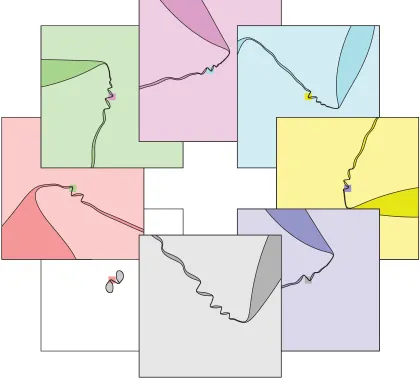
Approaching the singularity timets, the rapid acceleration of the evolution at the smallest scales means that the large-scale field becomes effectively frozen. The full evolution up to this time is presented in the Supplemental Material[18], which makes a continuous rescaling of the spatial variables by the instantaneous value of the maximum curvature κ. Near the final time of the integration t¼1.791 713 423 516 54, orts−t¼1.7×10⁻¹¹, the shape of the boundary is as shown in Fig. 3, where the series of panels depicts successive magnifications by a linear factor of 20 centered on the point of maximum curvature, each central shaded square being magnified in the adjacent panel of the same color. Despite differences in the details of the filament evolution, the large-scale structure at each level of magni-fication is remarkably uniform. Note that each magnimagni-fication appears rotated through a constant angle, implying a uniform angular velocity in the rescaled timeτ.
The physical cause and uniform scale reduction of the instability cascade may be understood from consideration of the stability properties of a single filament in the surface quasigeostrophic system. Linear growth rates for the filament instability scale as the inverse filament width: the inversion relation in Eq.(1)means that velocity values scale asθ0, which implies that the times taken for disturbances to grow to amplitudes comparable to the filament width are proportional to the filament width itself. We note that such a cascade is typically precluded in the two-dimensional vorticity equation because of the stabilizing effect of background shear on the growth of filament disturbances[19]and because growth rates do not increase as the filament width decreases. The independence of the rescaling factor on scale suggests that each instability is governed principally by the local shape of the patch in the vicinity of the filament. Because interactions in the quasigeostrophic model are more local than for the case of two-dimensional vortex dynamics, the evolution of a given filament is to a good approximation controlled by the influence of the parent filament that spawned it. However, the contribution to the velocity field by a local approximation to the contour integral, in fact, diverges logarithmically, meaning that the precise evolution requires consideration of the global patch shape. The dynamics is thus expected to be nonuniversal and may depend upon details of the initial conditions. Indeed, for initially elliptical patches, a variety of different evolutions is obtained for different values of the aspect ratio a. For large enough a, the evolution appears to remain smooth for all time; forain the range (0.17,0.19), the patch boundary develops a corner before disturbances of the central filament have time to grow to large amplitude; fora below about 0.12, a more complex combination of corner formation and filament instability occurs. A full description will be reported in a subsequent paper.
While a numerical demonstration can never be a sub-stitute for a rigorous mathematical proof, the present work provides the strongest evidence to date that the instability 1.75 1.76 1.77 1.78 1.79
t 101 102 103 104 106 108 1010
inverse filament width maximum curvature
0 5 10 15 20
τ 100 101 102 103 104 105 106 107 108 109 1010 1011 1012
[image:3.612.85.268.249.647.2]inverse filament width maximum curvature
FIG. 2. Maximum curvature and inverse filament width as a function of (a) timetand (b) rescaled timeτ¼−logðts−tÞ, with
ts¼1.791 713 423 533 387 8. Corresponding times in each panel
are indicated by the diamond symbols; the dashed lines indicate the function1=ðts−tÞ. Note the double-log scale in (a) and the
cascade may exist in the case of the temperature patch. The existence of such a cascade would, in turn, have implica-tions for the regularity problem of the quasigeostrophic equations when the initial θ is a smooth distribution in space, a problem about which very little is known. Because
θis conserved on fluid particles, a collapsing filament with
θsmoothly distributed across its width will retain its initial peak θ value at the filament center. As pointed out in Ref. [14], the filament boundary, or zero contour of the θ field, may be identified with the patch contour described above, in which case an instability cascade would again be expected to lead to the unbounded growth of ∇θ in finite time. This is in contrast to the case of the corner singularity of Ref.[16], which is intrinsic to the case of the temperature patch and which has no counterpart in the case of an initially smooth θ distribution. The present results suggest, therefore, that the evolution of the initially smooth θ distribution may also develop a singularity in finite time, an open problem of considerable theoretical interest.
*
[email protected]‑and.ac.uk
[1] J. G. Charney, Geofysiske publikasjoner17, 1 (1948). [2] B. J. Hoskins and F. P. Bretherton, J. Atmos. Sci. 29, 11
(1972).
[3] W. Blumen,J. Atmos. Sci.35, 774 (1978).
[4] I. M. Held, R. T. Pierrehumbert, S. T. Garner, and K. L. Swanson,J. Fluid Mech.282, 1 (1995).
[5] P. Constantin, A. J. Majda, and E. Tabak,Nonlinearity 7, 1495 (1994).
[6] P. Constantin,Physica (Amsterdam)86D, 212 (1995). [7] C. V. Tran, D. G. Dritschel, and R. K. Scott,Phys. Rev. E81,
016301 (2010).
[8] L. Onsager,Nuovo Cimento 6, 279 (1949).
[9] K. Ohkitani and M. Yamada,Phys. Fluids9, 876 (1997). [10] D. Cordoba,Ann. Math. 148, 1135 (1998).
[11] P. Constantin, Q. Nie, and N. Schorghofer,Phys. Lett. A
241, 168 (1998).
[12] J.-M. Hoyer and R. Sadourny,J. Atmos. Sci.39, 707 (1982). [13] R. T. Pierrehumbert, I. M. Held, and K. L. Swanson,Chaos
Solitons Fractals4, 1111 (1994).
[14] R. K. Scott,J. Fluid Mech.687, 492 (2011).
[image:4.612.96.516.49.429.2][15] M. N. Juckes,J. Atmos. Sci.52, 3247 (1995).
[16] M. A. Cordoba, D. Fontelos, A. M. Mancho, and J. L. Rodrigo, Proc. Natl. Acad. Sci. U.S.A. 102, 5949 (2005).
[17] D. G. Dritschel,Comput. Phys. Rep.10, 77 (1989).
[18] See Supplemental Material at http://link.aps.org/ supplemental/10.1103/PhysRevLett.112.144505for an ani-mation of the patch evolution in the rescaled time. [19] D. G. Dritschel, P. H. Haynes, M. N. Juckes, and