Sophie Smout1, Anna Rindorf2, Philip S. Hammond1, John Harwood1 and Jason
Matthiopoulos1,3
Modelling Prey Consumption and Switching by UK Grey Seals
1) NERC Sea Mammal Research Unit and Centre for Research into Ecological and
Environmental Modelling, Scottish Oceans Institute, University of St Andrews, St
Andrews KY16 8LB 2) DTU Aqua, Jægersborg Allé 1, DK-2920 Charlottenlund,
Denmark 3) Institute of Biodiversity, Animal Health and Comparative Medicine,
College of Medicine, Veterinary & Life Sciences, Graham Kerr Building, University
of Glasgow, Glasgow, G12 8QQ, Scotland, UK
Summary
12
Grey seals (Halichoerus grypus) are adaptable generalist predators whose diet
3
includes commercial fish species such as cod. Consumption by the seals may
4
reduce the size of some fish stocks or have an adverse effect on stock recovery
5
programmes, especially because predation may trap sparse prey populations in a
6
‘predator pit’ (Sinclair et al., 1998). To assess the likely impact of such effects, it
7
is important to know how consumption and consequent predation mortality
8
respond to the changing availability of prey. We present a model of grey seal
9
consumption as a function of the availability of multiple prey types (a
Multi-10
Species Functional Response – MSFR). We fit this MSFR to data on seal diet and
11
prey availability (based on the overlap between the distributions of predators and
12
prey). Bayesian methodology was employed to account for uncertainties in both
dependent and independent variables, improve estimation convergence by the use
1
of informative priors, and allow the estimation of missing data on prey
2
availability. Both hyperbolic (Type 2) and sigmoidal (Type 3) functional response
3
models were fitted to the data and the Type 3 model was clearly favoured during
4
model selection, supporting the conclusion that seal/prey encounter rates change
5
with prey abundance (sometimes referred to as ‘switching’). This suggests that
6
some prey species may be vulnerable to predator pit effects. The fitted model
7
reproduced contrasts in diet observed between different regions/years and,
8
importantly, added information to the prior distributions of prey abundance in
9
areas where the availability of some prey species (such as sandeels) was not
10
known. This suggests that the diet of predators such as seals could provide
11
information about the abundance and distribution of prey in areas that are not
12
covered by fisheries and research surveys.
13 14
Introduction
1516
Grey seals Halichoerus grypus consume a wide range of prey types in the North
17
Sea, including commercially valuable species such as cod, Gadus morhua
18
(Hammond and Grellier, 2006). In recent decades, the North Sea grey seal
19
population has grown considerably e.g. increasing by approximately 40% in the
20
decade 1999-2009 (Thomas, 2011; Newman et al., 2006). This has raised concerns
21
about competition with fisheries and possible conflicts between the conservation
22
of these charismatic predators and stock recovery programmes (Matthiopoulos et
23
al., 2008).
Estimating the net consumption of commercial fish by UK grey seals is therefore
1
important, and this has motivated a number of intensive diet studies for the North
2
Sea (Hall et al., 1998; Hammond et al., 1994; Hammond & Grellier 2006). These
3
studies show that there is significant variation across regions and seasons, and
4
between study years.
5 6
Because seals regularly return to rest at particular onshore haulout sites, their
7
access to offshore habitats is restricted by their need to remain in proximity to
8
these sites (Matthiopoulos et al., 2004). This imposes constraints on the
9
availability of prey and, as a result, seal diets appear to be related to prey
10
abundances in the region of these haulout sites (Prime and Hammond, 1990; Hall
11
et al., 1998; Hammond et al., 1994; Walton and Pomeroy, 2003). This suggests
12
that if we can obtain estimates of local prey abundance that are relevant to the
13
areas and dates for which diet is estimated, we can model the link between prey
14
consumption and prey availability. A model of the relationship between seal diet
15
and the availability of different prey types (a Multi-Species Functional Response -
16
MSFR) could be built using knowledge gained from ‘snapshot’ estimates of seal
17
diet based on samples collected in particular times and places. Such a model
18
could also be used to estimate consumption in years when diet studies were not
19
carried out, and to predict consumption rates if prey abundance changes as a
20
result of climate change or changes in the management of a fishery.The MSFR
21
could also form part of multi-species models that link the dynamics of separate
22
populations through their trophic interactions (Lindstrom et al., 2009).
The objective of this study was to estimate the parameters of a grey seal MSFR
1
using diet data collected during the 1980s and 2000s, together with estimates of
2
the availability of key prey types, based on catch-per-unit-effort (CPUE) data
3
from research and fishery trawls and seal telemetry data. We implemented a
4
Bayesian approach that takes account of uncertainty in both diet estimates and
5
prey availability.
6 7
Methods
89
In order to fit a model of consumption by North Sea grey seals, it was necessary to
10
address a number of important issues. First was an issue of model complexity.
11
Grey seals are generalist predators, and more than 100 prey species have been
12
recorded in the diet of our study population. We needed to decide how many prey
13
types should be included in the MSFR, given that the data available to fit the
14
model were limited by the number of seal diet sampling occasions, and the
15
availability of fish survey data.
16 17
Second, it was important to estimate prey availability on an appropriate spatial
18
scale, given that the foraging range of seals is limited by their dependence on
19
coastal haulout sites. Three long term data sets were used to tackle this
20
estimation. Data from the IBTS (International Bottom Trawl Survey) for demersal
21
fish species and Danish fishery-based records of fishing effort and catches for
22
sandeels were used to create spatial models of prey distribution. We then
23
estimated the availability of prey to grey seals at given offshore locations by
24
comparing predictions of the usage of these locations by seals, derived from a
model of the way they use space at sea that was based on telemetry data
1
(Matthiopoulos et al., 2004), with predicted distributions of the different prey
2
types derived from the fisheries data sets.
3 4
Finally, we needed to account for the uncertainty associated with the estimates
5
of diet and prey availability. This required a flexible modelling approach that was
6
able to propagate uncertainty through the estimation process, so that it was
7
represented in the precision of final parameter estimates and inferences. Key
8
steps in our modelling are represented in Figure 1 and described in more detail
9
below.
10 11
1. Diet composition 12
Diet composition was known from previous grey seal diet surveys, based on the
13
analysis of fish otoliths in seal faecal samples (scats) (Hammond and Prime, 1990;
14
Prime and Hammond, 1990; Hammond and Grellier, 2005; Hammond et al., 1994).
15
Samples were collected at North Sea haul-out sites during the 1980s and in 2002.
16
The majority of the 1980s data were from 1985 but there were also some data
17
from the Farne Islands and the Isle of May in 1983-1988, which we treated as if
18
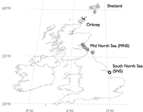
they were representative of 1985. All diet samples were aggregated according to
19
four geographical groupings (Figure 2): Shetland (where data were available for
20
2002 only), Orkney, Mid North Sea (including seal haulouts at the Isle of May,
21
Abertay, and the Farnes) and South North Sea (including a major seal haulout site
22
at Donna Nook). For this analysis we used Quarter 1 diet estimates from the 1985
23
samples, and Quarter 1 and 3 estimates from the 2002 samples, based on the
availability of matching prey abundance data (see below). We only made use of
1
scat collections containing > 15 faecal samples (Grellier, 2006). This resulted in 11
2
diet estimates in all, each corresponding to a unique combination of year (2002 or
3
1985), haulout group, and date (Quarter 1 or Quarter 3). In total, 1370 separate
4
scat samples contributed to the analysis. Uncertainty in diet composition was
5
estimated using a combination of parametric and non-parametric random
6
sampling (Hammond and Rothery, 1996).
7 8
One particular difficulty in the interpretation of grey seal diet data arises from
9
the fact that partially-digested otoliths from sandeels are difficult to identify to
10
species on the basis of morphology. In the diet analyses, all sandeel species are
11
therefore grouped but the large size of some otoliths in the scat samples implies
12
they are from the greater sandeel Hyperoplus lanceolatus rather than from the
13
more abundant Ammodytes marinus (Prime & Hammond, 1990; Hammond et al
14
1994a, Hammond & Prime 1990; Hammond & Grellier 2006),which is the object of
15
North Sea commercial fisheries. Based on an examination of the size distributions
16
of A. marinus caught by the fishery, it was decided that sandeels whose length
17
was estimated to be less than 20cm long were probably A. marinus. We
18
estimated that 82% of all sandeel biomass consumed in 2002 and 53% of all
19
sandeel biomass consumed in the 1980s samples was A. marinus.
20 21
Only prey types that contributed more than 5% to the observed diet in two or
22
more collections were included in the analysis.
2. Prey availability
1 2
Catch per unit effort (CPUE) data were available from the International Bottom
3
Trawl Surveys for the North Sea for both study years (1985 and 2002), for Quarter
4
1. In 2002, Quarter 3 data were also available. The geographic location for the
5
start point of each trawl was known, and multiple surveys were performed in each
6
statistical rectangle (IBTSWG, 2010). Localised polynomial smoothing (Bowman
7
and Azzalini, 1997) was used to interpolate IBTS CPUE data over a grid with 5km
8
resolution. The availability of each prey type to seals at each of the four haul-out
9
groups was calculated by weighting the prey distribution using an accessibility
10
surface derived from a model of the accessibility of space at sea to grey seals
11
from the different haulout sites (Matthiopoulos, 2003) as follows:
12 13
Ni,j = sk,jfk,i
k
∑
(1) Where:Ni,j availability of prey type i to seals at haulout j sk,j accessibility of grid cell k to seals from haulout j
fk,i relative abundance of prey type i in cell k
14
15
Means and variances forNi,j were obtained by bootstrap re-sampling from the IBTS 16
data, with overlap between fish distribution and seal usage re-calculated for each
17
sample. Typical spatial distributions of seals and fish are illustrated in Figure 3.
18 19
Sandeel are not well represented in IBTS survey catches, so it was difficult to
20
estimate their distribution robustly based on this data set. This was especially the
21
case when we wished to determine temporal changes in sandeel abundance,
because data could not be aggregated across years. However, there were catch
1
records from the Danish sandeel fleet for some locations. In contrast to scientific
2
surveys, commercial catches do not cover all areas in all years, and it was
3
therefore not possible to estimate a separate spatial distribution each year using
4
these data. To obtain a complete time series of local abundance estimates (i.e.
5
for all fished locations and all years) we therefore had to assume that the
6
distribution of sandeel remained constant over the years. An index of the average
7
density of sandeels within each foraging area was obtained from catch per unit
8
effort analysed in a Generalised Linear Model (GLM). The catch C (in tonnes per
9
day) in a statistical rectangler (0.5° latitude by 1° longitude) for a vessel of gross
10
tonnage G in year y and quarter qwas given by:
11 12
ln( ˆCr,q,y,GT)=αq,r+βq,y+γqln(G) (2)
13
14
The parameters α, β, and γ were estimated separately for each quarter of the
15
year. Observations were taken from Danish logbook records of the catch of
16
sandeel per day for the years 1982 to 2010, in tonnes. α accounts for the average
17
quarterly spatial distribution of sandeel CPUEs within each area, βaccounts for
18
yearly differences in the North Sea average quarterly CPUE and γ is a factor
19
accounting for the increase in CPUE with vessel size. A standard vessel size of
20
G=200GT was then assumed, and the model was used to estimate an index of
21
sandeel biomass within each foraging area by ICES statistical rectangle, year and
22
quarter. Because the sandeel fishery mainly takes place from April to August, it
23
was only possible to produce estimates for Quarters 2 and 3. To assure accuracy
of the results, predictions were only made for areas, years and quarters where
1
more than five logbook records were available.
2 3
Where possible, the sandeel model was used to make predictions in those ICES
4
rectangles that were located closest to the haulout sites used for scat collections.
5
Weighted means of the sandeel abundance in those local rectangles were
6
calculated, based on the maps of the accessibility of space to seals. For haulout
7
site j, the weight accorded to the CPUE estimate from rectangle r was calculated
8
as
9
wr,j =
skr,j kr
∑
wr,j r
∑
(3)10
Where kr is the set of grid cells inside ICES rectangle r.
11 12
Uncertainties in these estimates were based on the standard deviation for CPUE
13
estimates produced by the GLM model (equation (2)). For haulouts where sandeel
14
predictions were not available (Orkney and Shetland in 1985 and 2002) unknown
15
abundances were estimated during the model fitting process, and further details
16
are given below.
17 18
3. Fitting the model
19 20
The following flexible expression was used to represent the seal functional
21
response. This can take the form of a Holling type 1, 2 or 3 response depending on
22
the values of parameters a, t and m (Real, 1977; Holling, 1959).
1
ci= aiNimi
1+ a jt jN jm j
j
∑
(4)
2
3
ci represents the consumption rate of prey i by a single seal, Ni is the availability
4
of prey type I, ti is the time taken to consume an item of prey i, ai is a parameter
5
that described the rate at which seals encounter prey i, and mi is a shape
6
parameter. If m=1 for a given prey type, the conditional functional response for
7
that prey is hyperbolic (Type 2). If m>1, the functional response is sigmoidal
8
(Type 3) with an inflexion at low prey density.
9 10
On their own, the seal scat data can be used to estimate diet composition but not
11
consumption rates. Therefore, we recast the model in terms of diet composition
12
so that predicted proportions could be compared with observed proportions in
13
order to fit the model. Equation (4) can be readily adapted for this purpose,
14
because the denominator of the equation is the same for all prey types, giving:
15
16
ci c j j
∑
= aiNimi
a jN jm j j
∑
(5)
17
18
Two models were fitted to the data. In Model 1, the value of the parameter m was
19
set at 1 for all prey, corresponding to a hyperbolic or Type 2 functional response.
We based Model 2 on the results of experiments with captive seals (Gallon, 2008),
1
and assigned a fixed value of 1.5 to the parameter m for all prey types,
2
corresponding to a sigmoidal or Type 3 functional response.
3 4
Equation (5) holds true not only when absolute densities are used but also when
5
all densities are scaled by an identical constant. Thus the relative values of ai are
6
sufficient to predict diet composition, but only relative values can be estimated
7
when the function is fitted to data. Further, the abundance of any prey type can
8
be arbitrarily multiplied by a constant value if the corresponding encounter rate
9
parameter is also divided by the same value. It is therefore possible to use prey
10
availability indices rather than absolute estimates of biomass or numbers,
11
provided we can assume the indices are proportional to true prey abundance. To
12
facilitate the numerical performance of the fitting process, all prey abundance
13
indices were re-scaled before fitting the model so that the maximum observed
14
value of abundance for any prey type was 100.
15 16
Prey types not directly included in the model generally contributed less than 15%
17
to the seal diets. These prey types were aggregated into a single class titled
18
‘other prey’. The proportion of ‘other prey’ in the diet was estimated in the same
19
way as the proportion of specific prey types. The abundance of ‘other prey’ in the
20
environment was assumed to be constant over time, because it is the aggregate of
21
a large number of near-independent time series whose total is unlikely, on
22
average, to vary systematically.
Models 1 and 2 were fitted using a Markov chain Monte Carlo algorithm (MCMC)
1
coded in WinBugs (Lunn et al., 2000). Random values of prey availability were
2
drawn from zero-truncated Normal distributions for each prey type at each step in
3
the Markov chain, with mean and variance parameters estimated from
4
bootstrapping. Where no estimate of sandeel abundance was available, a prior
5
N(50,20) distribution for sandeel availability was assumed, so that sandeel
6
abundance was effectively estimated in those areas as though it was a further
7
unknown parameter. The abundance of ‘other prey’ was set at 100 in all areas
8
and for all dates. A Normal distribution was used to compare the model
9
predictions of diet composition with the empirical values; the variance of this
10
distribution was based on the estimated uncertainty in the original diet estimates.
11
It was assumed the errors in predictions were conditionally independent once the
12
relationship between proportions in the diet had been accounted for in the
13
model.
14 15
There are few direct observations of grey seals foraging in their natural habitat
16
(Bowen et al., 2002). It was thus difficult to obtain estimates of encounter rates
17
in order to create informative priors for a. Only relative values of a could be
18
estimated, so the value of a for sandeels was fixed at 1, while a’s for all other
19
species were estimated based on wide uniform priors ai ~ U(0,10). Results were
20
tested for sensitivity to the assumed width of the uniform prior for a.
In each case, the MCMC was run for 100,000 iterations after a burn-in of 10000
1
iterations. Two parallel Markov chains were examined for mixing and
2
convergence.
3 4
Results
56
Twelve prey types, shown in Table 1 were identified. Herring and sprat were
7
included because of their interest to commercial fisheries, while dragonet and sea
8
scorpion were included because of their important role in seal diets in some
9
locations. A number of prey types, such as cod and sandeel, are important both to
10
seals and commercial fisheries.
11 12
The MCMC converged successfully for both Model 1 and Model 2. DIC suggests that
13
the Type 3 functional response model (Model 2, with DIC=706) is preferred to
14
Model 1 (DIC=760). We also compared the two models by estimating the Bayes
15
factor (King et al., 2009), which was 5.4 x 10¹¹, again suggesting that Model 2 is
16
strongly favoured. Only results from Model 2 are reported from now on. Marginal
17
posterior distributions are shown in Figure 4, and mean estimates and standard
18
deviations in Table 1.
19 20
Table 1: Posterior marginal mean of the encounter rate parameter a for each
21
prey type, based on 1000 samples from the Markov chain (95% Bayesian credible
22
intervals are shown in brackets). These are relative values, with the value for
23
sandeels fixed at 1.
PREY TYPE a
Cod Gadus morhua 0.461 (0.337,0.594)
Whiting Merlangius merlangus 0.197 (0.143,0.253)
Saithe Pollachius virens 0.152 (0.0954,0.213)
Haddock Melanogrammus aeglefinus 0.111 (0.00558,0.367)
Norway Pout Trisopterus esmarkii 0.0572 (0.00244,0.129)
Plaice Pleuronectes platessa 0.101 (0.0463,0.148)
Herring Clupea harengus 0.0659 (0.0130,0.121)
Dover Sole Solea solea 0.210 (0.124,0.303)
Sprat Sprattus sprattus 0.0607 (0.00409,0.142)
Dragonet Callionymus lyra 0.612 (0.480,0.770)
SeaScorpion Myocephalus scorpius 0.700 (0.527,0.916)
Sandeel Ammodytes marinus 1 (fixed value)
Other prey 0.450 (0.399,0.500)
1
The posterior distributions of the parameters (Figure 4) were well defined and
2
were insensitive to the choice of priors, provided these were wide enough. The
3
U(1,10) distribution was sufficiently wide.
4 5
Missing prey data were also estimated. Figure 5 shows the prior and posterior
6
distributions for sandeel abundance in Orkney in 2002.
7 8
Diet predictions based on the fitted model compared well with original diet
9
estimates from scat data for contrasting years and locations. For example, they
captured the shift in diet due to the increased abundance of the benthic species
1
(principally dragonet and sea scorpion) in the Southern North Sea in 2002 (Figure
2
6).
3 4
Modelled relationships between diet and prey availability are illustrated in Figure
5
7 for cod and sandeels. For these (and other) species, there is a strong effect of
6
general prey abundance on diet. When alternative prey is plentiful, the
7
consumption of focal prey may be considerably reduced (here we assume that
8
seals consume an approximately consistent daily mass of fish, such that the
9
contribution of a prey to the diet is directly proportional to the mass of that fish
10
consumed). Sandeel availability, in particular, had a strong effect on the
11
consumption of other prey types. The effect of both cod and sandeel abundance
12
on the consumption of cod, when all other prey types were held at constant
13
availability, is shown in the right hand panel of Figure 8. Sandeel has a strong
14
effect on consumption rates for cod, in contrast to the interaction between cod
15
consumption and haddock availability (left hand panel of Figure 8). All plots are
16
based on prey availabilities that fall within the historical range of the data.
17 18
Figure 9 compares predicted seal predation and fishery removals of cod (both in
19
the cod fishery itself, and in fisheries targeting other species). The aim of the
20
current recovery programme for North Sea cod stocks is to increase levels of
21
spawning stock biomass - SSB (ICES, 2012). We used a target level of SSB=150,000
22
tonnes to ‘scale up’ the cod distribution from 2002; i.e. we assumed that the
23
spatial distribution of seals and cod will remain unchanged from its 2002 values
when the cod stock recovers. If the cod abundance in a given region in 2002 is
1
Nr,2002 and it will increase to qNr,2002 , where q=150000/42574, the ratio of target
2
cod SSB in the North Sea to the estimated SSB in 2002 (ICES, 2012). We further
3
assume that the North Sea grey seal population and all other prey types will
4
remain at their 2002 levels. The predicted net consumption of cod by grey seals in
5
the North Sea is then given by the predicted consumption at each of the main scat
6
collection haulout sites, multiplied by the number of seals whose foraging is
7
associated with that haul out site (Hammond and Grellier, 2005). We can obtain
8
an indication of the predicted relative importance of these sources of mortality
9
by comparing the historical levels of removals due to fishing and the predicted
10
seal removals.
11 12
To further investigate possible conflicts between seal predation and the cod
13
fishery, we plotted the predicted relationship between mortality induced by seal
14
predation, and cod abundance. Figure 10 shows this plot which is based on the
15
estimated model parameters and assumes that all other prey types remain at
16
constant average levels. Over the range of observed cod availabilities in our data,
17
the figure shows that seal predation mortality increases with the size of the cod
18
stock. The implications of this are discussed below.
19 20
Discussion
2122 23
The MSFR used in this study is simple and excludes some potentially interesting
24
biological processes such as competition between predators (Abrams and
Ginzburg, 2000) and individual differences in diet and encounter rates (Beck et
1
al., 2007). These simplifications do, however, limit the number of parameters to
2
be estimated, making it feasible to fit the model to our data set. They are also
3
consistent with approaches used in other studies of generalist marine predators
4
(Koen-Alonso and Yodzis, 2005; Lewy and Vinther, 2004). Given that the focus of
5
this exercise was to make general inferences about interactions between seal
6
populations and fish stocks, we aimed to model consumption for a ‘typical’ seal.
7 8
The choice of prey types to be modelled was based on a simple criterion. Other
9
selection approaches might be used, and these could result in different
10
combinations of key prey types. This would alter what the model can predict,
11
because seal consumption of a prey species whose availability is not explicitly
12
modelled cannot be predicted. Grey seals are generalists, so it is possible that
13
one or more of the prey types we have grouped into the ‘other prey’ category
14
might become an important element of seal diets under a different regime of prey
15
availability. The model should therefore not be used to make predictions for
16
scenarios that involve major shifts in prey abundance, well outside those observed
17
in the North Sea over the past three decades.
18 19
The MSFR enables us to predict how consumption of any given prey type is likely
20
to be influenced by the availability of alternative prey. It appears that sandeel
21
abundance may have a particularly strong effect on the consumption of other
22
species. In years such as 2003 when sandeel stock levels in the North Sea were
very low, we expect that grey seals will have changed their diet, increasing their
1
intake of other prey in response to the sandeel shortage.
2 3
The favoured model involved a sigmoidal or Type 3 functional response. This
4
implies that it is possible for grey seals to keep some prey types below a critical
5
density, because predator-induced mortality increases with prey abundance at
6
low levels of abundance, creating what is known as a ‘predator pit’ (Sinclair et
7
al., 1998). Figure 10 does show a positive relationship between grey seal
8
predation mortality on cod, and cod abundance, over the range of abundances we
9
observe in our data, and this suggests the possibility of a predator pit effect for
10
cod induced by seals in the North Sea. However, Figure 9 indicates that,
11
historically, seal predation removed substantially less cod than the fisheries over
12
a wide range of cod abundance, suggesting it is not probable that seal predation
13
has been a crucial factor in reducing the size of this stock to recent low levels.
14
Further, the occurrence of a predator pit, even in a simple system involving a
15
specialist predator that consumes only one prey, is critically dependent on the
16
nature of density dependence in the prey’s per capita reproductive rate. In a
17
multi-species system like the North Sea, the effects of seal predation on the cod
18
stock will be strongly influenced by other factors too, especially other sources of
19
mortality for cod. Seals are operating within a complex food-web, and indirect
20
effects may result if the prey of seals are also predators of one another (as, for
21
example, is the case for cod and haddock). It is therefore difficult to make
22
reliable predictions about the long-term consequences of predatory interactions
23
between grey seals and any one type of prey based on the seal MSFR alone. To
evaluate the likely role of grey seals in fish stock dynamics, such as their effect
1
on stock recovery programmes, the MSFR should be included as part of a
multi-2
species population dynamics model that includes all the main species in the
3
system. Such models are also able to include spatial aspects, so that seal
4
predation could be attributed to appropriate areas of the North Sea (Lewy and
5
Vinther, 2004; Lindstrom et al., 2009). Detailed modelling of the use of space by
6
grey seals and fish may also provide more robust predictions of these
predator-7
prey interactions (Aarts et al., 2008).
8 9
We were able to estimate missing prey abundance data as part of the process of
10
fitting the MSFR (Figure 5). This suggests another way in which top predators can
11
be used as indicators of ecosystem state (Cury et al., 2011) because it provides a
12
methodology for converting information on their diet into estimates of prey
13
abundance in areas where direct surveys are difficult to conduct and for
14
reconstructing historical time series of prey abundance, when long-term faecal
15
data sets are available.
16
17
Acknowledgements
18
Research by Sophie Smout and Anna Rindorf was supported by the EU-FP7 grant
19
FACTS, reference 244966
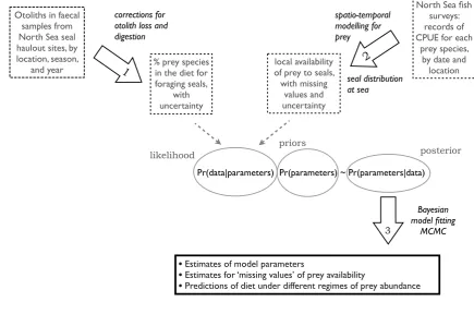
Figure 1: Steps in the modelling carried out for this paper. Step 1: faecal (scat)
1
samples are processed and otolith measurements analysed to reconstruct seal
2
diets. Step 2: catch per unit effort (CPUE) data are used to fit models of the
3
distribution of prey in time and space. These are combined with at-sea
4
distribution of seals to produce an index of predator-prey overlap, taken to
5
represent the availability of prey to seals. Step 3: Bayesian methodology is used
6
to fit a model of prey preference and switching to the diet composition and prey
7
availability data. Uncertainty estimates from steps 1 and 2 are carried through to
8
inform the model-fitting in step 3, and influence the final estimates of
9
uncertainty in parameters and predictions of the MSFR model.
10
Otoliths in faecal samples from North Sea seal haulout sites, by location, season,
and year % prey species in the diet for foraging seals,
with uncertainty corrections for otolith loss and digestion
North Sea fish surveys: records of CPUE for each
prey species, by date and
location local availability
of prey to seals, with missing
values and uncertainty
spatio-temporal modelling for prey
2
seal distribution at sea
•Estimates of model parameters
•Estimates for ‘missing values’ of prey availability
•Predictions of diet under different regimes of prey abundance priors
Bayesian model fitting
MCMC
3
Pr(data|parameters) Pr(parameters) ~ Pr(parameters|data)
likelihood posterior
1
Figure 2: Haulout sites where faecal sampling was carried out. Abbreviations: SNS
1
southern North Sea, MNS mid North Sea.
2
Figure 3: Accessibility of space to grey seals foraging from local haulout sites in
1
the mid-North Sea shown on a log scale (left hand panel). Distribution of cod in
2
the North Sea based on smoothed CPUE for Quarter 1, 1985 (right hand panel).
3
These results, and similar results for other prey types and haulout areas, were
4
used to estimate the availability of prey to grey seals. The abundance of prey
5
close to the seals’ haulout sites will have greater influence on the calculated
6
availability than the abundance of more distant prey.
7
Figure 4: Posterior distributions for the encounter rate parameter a. The prey
1
species are: (1) cod, (2) whiting, (3) saithe, (4) haddock, (5) Norway pout, (6)
2
plaice, (7) herring, (8) Dover sole, (9) sprat, (10) dragonet, (11) sea scorpion, and
3
(12) other prey. The prior distribution in each case was U(0,10). The encounter
4
rate for sandeels was fixed at the value 1.
5
6
Figure 5: Prior (smooth curve) and posterior (histogram) distributions of sandeel
7
abundance in Orkney in Quarter 1 of 2002, an area/date combination for which no
8
sandeel CPUE survey data were available
9
CPUE Sandeels Orkney 2002 Q1
Frequency
0 50 100 150
0
50
100
150
200
[image:23.595.109.297.499.654.2]Figure 6: Model predictions (upper panel) of grey seal diet and direct estimates
1
(lower panel, Hammond & Grellier 2006) based on scat samples collected at two
2
contrasting sites (ORK = Orkney; SNS = southern North Sea).
3
Predic'on*1985*ORK*Q1*
Cod$ Whi(ng$ Haddock$ Saithe$ NorwayPout$ Plaice$ Herring$ DoverSole$ Sprat$ Dragonet$ SeaScorpion$ Amarinus$
Predic'on*2002*SNS*Q3*
Cod$ Whi(ng$ Haddock$ Saithe$ NorwayPout$ Plaice$ Herring$ DoverSole$ Sprat$ Dragonet$ SeaScorpion$ Amarinus$
Diet%1985%ORK%Q1%
Cod$ Whi(ng$ Haddock$ Saithe$ NorwayPout$ Plaice$ Herring$ DoverSole$ Sprat$ Dragonet$ SeaScorpion$ Amarinus$
Diet%2002%SNS%Q3% Cod$
Whi(ng$ Haddock$ Saithe$ NorwayPout$ Plaice$ Herring$ DoverSole$ Sprat$ Dragonet$ SeaScorpion$ Amarinus$ Other$
Figure 7: Variation of seal diet with prey availability shown as a single-species plots for cod and 1
sandeels, with two different levels for the availability of all other prey types. The contribution of 2
cod/sandeels to the diet was lower when alternative prey abundance was high (cyan), and higher 3
when alternative prey abundance was low (black). 4
0 20 40 60 80 100
0 10 20 30 40 50 60 70 abundance index
% Sandeel in diet
0 20 40 60 80 100
0 10 20 30 40 abundance index
% Cod in diet
alternative prey at low abundance
alternative prey at high abundance
5
Figure 8: The effect of prey availability on cod consumption by grey seals, taking account of the 6
availability of haddock (left hand panel), and sandeels (right hand panel) as alternative prey. The 7
abundance of all other prey types was held at constant (low) values. The colour scale represents 8
the proportion (by weight) of seal diet that is comprised of cod. 9
20 40 60 80 100
20 40 60 80 100 Cod Haddock 0.05 0.10 0.15 0.20 0.25 0.30
% Cod in seal diet
20 40 60 80 100
50 60 70 80 90 100 Cod Amar in us 0.05 0.10 0.15 0.20 0.25 0.30
% Cod in seal diet
[image:25.595.98.473.550.707.2]Figure 9: Predicted removals of cod by seals (black line) and by commercial
1
fisheries (circles) for the whole North Sea at different levels of Spawning Stock
2
Biomass (SSB). Model predictions assumed that the spatial distribution of cod did
3
not change over time. Average abundances of alternative prey were assumed for
4
each area, but cod abundance was scaled up starting at 2002 levels and increasing
5
to target levels for MSY-based management (Bpa). Consumption by seals was
6
summed over the four main areas (Shetland, Orkney, Mid and South North Sea),
7
assuming 2002 population levels for the seals. Published estimates were used to
8
plot removals by fisheries (for both cod and other species) and corresponding to
9
SSB.
10
● ●
●
● ●
● ● ● ● ●
● ● ● ●
● ● ●●
Cod SSB (1000 tonnes)
Remo
vals (1000 tonnes)
40 60 80 100 120
0
80
160
240
Figure 10: Model predictions of the variation in seal-induced cod mortality as a
1
function of cod abundance. The quantity plotted on the y axis is (consumption
2
rate)/(cod abundance) and it is thus proportional to the mortality rate for cod.
3
Cod abundance is in arbitrary units (see text) and is assumed to be proportional to
4
true abundance. The maximum value of cod abundance in our data set is 100.
5
● ●
● ● ●
● ●
● ●
● ●
Scaled Cod abundance
Scaled Mor
tality
0
100
200
300
400
500
0.00
0.10
0.20
0.30
1
Bibliography 2
3
Aarts, G., MacKenzie, M., McConnell, B., Fedak, M., and Matthiopoulos, J. 2008. Estimating space-4
use and habitat preference from wildlife telemetry data. Ecography, 31: 140-160. 5
Abrams, P. A., and Ginzburg, L. R. 2000. The nature of predation: prey dependent, ratio 6
dependent or neither? Trends in Ecology & Evolution, 15: 337-341. 7
Beck, C. A., Iverson, S. J., Bowen, W. D., and Blanchard, W. 2007. Sex differences in grey seal 8
diet reflect seasonal variation in foraging behaviour and reproductive expenditure: evidence from 9
quantitative fatty acid signature analysis. Journal of Animal Ecology, 76: 490-502. 10
Bowen, W. D., Tully, D., Boness, D. J., Bulheier, B., and Marshall, G. 2002. Prey-dependent 11
foraging tactics and prey profitability in a marine mammal. Marine Ecology Progress Series, 244: 12
235-245. 13
Bowman, A. W., and Azzalini, A. 1997. Applied Smoothing Techniques for Data Analysis: the Kernel 14
Approach with S-Plus illustrations, Oxford University Press, Oxford. 15
Cury, P. M., Boyd, I. L., Bonhommeau, S., Anker-Nilssen, T., Crawford, R. J. M., Furness, R. W., 16
Mills, J. A., et al. 2011. Global Seabird Response to Forage Fish Depletion-One-Third for the Birds. 17
Science, 334: 1703-1706. 18
Gallon, S. 2008. Foraging strategies in grey seals (Halichoerus. grypus) : foraging effort and prey 19
selection. PhD Thesis, St Andrews University. 20
Grellier, K. 2006. Grey Seal Diet in the North Sea. PhD Thesis, University of St Andrews. 21
Hall, A. J., Watkins, J., and Hammond, P. S. 1998. Seasonal variation in the diet of harbour seals 22
in the south-western North Sea. Marine Ecology-Progress Series, 170: 269-281. 23
Hammond, P. S., and Grellier, K. 2005. Grey seal diet composition and fish consumption in the 24
North Sea. Report for the Department for Environment, Food and Rural Affairs: 1-54. 25
Hammond, P. S., Hall, A. J., and Prime, J. H. 1994. The Diet of Grey Seals around Orkney and 26
Other Island and Mainland Sites in North-Eastern Scotland. Journal of Applied Ecology, 31: 340-27
350. 28
Hammond, P. S., and Prime, J. H. 1990. The diet of British grey seals (Halichoerus grypus). In
29
Population biology of sealworm (Pseudoterranova decipiens) in relation to its intermediate and 30
seal hosts. (Canadian Bulletin of Fisheries and Aquatic Sciences). pp. 243-254. Ed. by W. D. 31
Bowen. 32
Hammond, P. S., and Rothery, P. 1996. Application of computer sampling in the estimation of seal 33
diet. Journal of Applied Statistics, 23: 525-533. 34
Holling, C. S. 1959. The components of predation as revealed bu a study of small mammal 35
predation of the European pine sawfly. Canadian Entomologist, 91: 293-320. 36
ICES. 2012. Report of the Working group on the Assessment of Demersal Stocks in the North Sea 37
and Skagerrak. 38
IBTSWG 2010 Manual for the International Bottom Trawl Surveys. ICES, Copenhagen. 39
King, R., Morgan, B. J. T., Gimenez, O., and Brooks, S. P. 2009. Bayesian Analysis for Population 40
Ecology, Chapman and Hall. 41
Koen-Alonso, M., and Yodzis, P. 2005. Multispecies modelling of some components of the marine 42
community of northern and central Patagonia, Argentina. Canadian Journal of Fisheries and 43
Aquatic Sciences, 62: 1490-1512. 44
Lewy, P., and Vinther, M. 2004. . A stochastic age-length-structured multispecies model applied to 45
North Sea stocks. Ices cm, 2004/FF:20. 46
Lindstrom, U., Smout, S., Howell, D., and Bogstad, B. 2009. Modelling multi-species interactions in 47
the Barents Sea ecosystem with special emphasis on minke whales and their interactions with cod, 48
herring and capelin. Deep-Sea Research Part Ii-Topical Studies in Oceanography, 56: 2068-2079. 49
Lunn, D. J., Thomas, A., Best, N., and Spiegelhalter, D. 2000. WinBUGS - A Bayesian modelling 50
framework: Concepts, structure, and extensibility. Statistics and Computing, 10: 325-337. 51
Matthiopoulos, J. 2003. The use of space by animals as a function of accessibility and preference. 52
Ecological Modelling, 159: 239-268. 53
Matthiopoulos, J., McConnell, B., Duck, C., and Fedak, M. 2004. Using satellite telemetry and 54
aerial counts to estimate space use by grey seals around the British Isles. Journal of Applied 55
Matthiopoulos, J., Smout, S., Winship, A. J., Thompson, D., Boyd, I. L., and Harwood, J. 2008. 1
Getting beneath the surface of marine mammal - fisheries competition. Mammal Review, 38: 167-2
188. 3
Newman, K. B., Buckland, S. T., Lindley, S. T., Thomas, L., and Fernandez, C. 2006. Hidden 4
process models for animal population dynamics. Ecological Applications, 16: 74-86. 5
Prime, J. H., and Hammond, P. S. 1990. The Diet of Gray Seals from the South-Western North-Sea 6
Assessed from Analyses of Hard Parts Found in Feces. Journal of Applied Ecology, 27: 435-447. 7
Real, L. 1977. The kinetics of the functional response. American Naturalist, 111: 289-300. 8
Sinclair, A. R. E., Pech, R. P., Dickman, C. R., Hik, D., Mahon, P., and Newsome, A. E. 1998. 9
Predicting effects of predation on conservation of endangered prey. Conservation Biology, 12: 564-10
575. 11
Thomas, L. 2011. Estimating the size of the UK grey seal population between 1984 and 2010. 12
Report for the Special Committee on Seals. 13
Walton, M., and Pomeroy, P. 2003. Use of blubber fatty acid profiles to detect inter-annual 14
variations in the diet of grey seals Halichoerus grypus. Marine Ecology-Progress Series, 248: 257-15
266. 16