On the long time integration of stochastic gradient systems

On the long-time integration of stochastic gradient systems

B. Leimkuhler

, C. Matthews

and M.V. Tretyakov

July 7, 2014

Abstract

This article addresses the weak convergence of numerical methods for Brownian dynamics. Typical analyses of numerical methods for stochastic differential equations focus on properties such as the weak order which estimates the asymptotic (stepsize h →0) convergence behavior of the error of finite time averages. Recently it has been demonstrated, by study of Fokker-Planck operators, that a non-Markovian numerical method [Leimkuhler and Matthews, 2013] generates approximations in the long time limit with higher accuracy order (2nd order) than would be expected from its weak convergence analysis (finite-time averages are 1st order accurate). In this article we describe the transition from the transient to the steady-state regime of this numerical method by estimating the time-dependency of the coefficients in an asymptotic expansion for the weak error, demonstrating that the convergence to 2nd order is exponentially rapid in time. Moreover, we provide numerical tests of the theory, including comparisons of the efficiencies of the Euler-Maruyama method, the popular 2nd order Heun method, and the non-Markovian method.

1

Introduction

Stochastic gradient systems are stochastic differential equations inddimensions having the form

dX =a(X)dt+σdw, X(0) = X0, (1.1)

where

a(x) :=−∇V(x), (1.2)

V(x),x∈Rd, is a potential energy function andσ >0 is a constant which characterizes the strength of the additive noise, here described by a standardd-dimensional Wiener process w(t). These systems originate in the work of Einstein [5, 6] to describe the motion of Brownian particles. They arise in mathematical models for chemistry, physics, biology and other areas, when the cumulative effect of unresolved degrees of freedom must be incorporated into a model to ensure its physical relevance. Under mild conditions on V, the system (1.1) is ergodic [8, 13] and has the unique invariant distribution ρβ ∝ exp(−βV),

whereβ= 2σ−2_{. Numerical methods for solving the equation (1.1) compute a discrete sequence of states} X1,X2, . . . by iteratively approximating the short time evolution. The error in the numerical solution is typically quantified in either a strong sense (accuracy with respect to a particular stochastic path associated to (1.1)) or by reference to an evolving distribution (weak error, or error in averages); the latter is the focus of this article. Ideally, the discrete states are ultimately distributed in a way that is consistent with the invariant distribution, but for complex applications the introduction of error in the numerical process is inevitable. In this article we examine the asymptotic (t→ ∞) behavior of the weak error.

Undoubtedly, the most common numerical method for solving (1.1) is the Euler-Maruyama method which approximates X(tk),tk =hk, by the iteration

Xk+1= Xk+ha(Xk) +σ

√

hξk+1, (1.3)

∗_{School of Mathematics and the Maxwell Institute for Mathematical Sciences, University of Edinburgh, Kings Buildings,}

Mayfield Road, Edinburgh, EH9 3JZ, UK

†_{School of Mathematical Sciences, University of Nottingham, Nottingham, NG7 2RD, UK. Email:}

whereξk = (ξk1, . . . , ξkd)> andξki, i= 1, . . . , d, k= 1, . . . ,are i.i.d. random variables with the lawN(0,1).

For analysis of the weak error, one considers a finite time interval [0, τ], withτ =hN. The probability measure associated to (1.1) is described by a probability density ρ(t, x) that evolves according to the Fokker-Planck equation

∂ρ ∂t =L

†_ρ,

whereL† _{is the adjoint (in theL}

2 sense) of the generator for (1.1), defined by

L:=

d

X

i=1

ai(x) ∂

∂xi +

σ2 2

d

X

i=1

∂2

(∂xi₎2. (1.4)

The solutionρ(t, x) evolves from an initial probability distributionρ(0, x) to the steady stateρ(∞, x) =

ρβ. Letϕbe a test function (such as an element of the Schwartz space ofC∞functions rapidly decaying

at infinity). Then the average ofϕat time τ may be taken to be

¯

ϕ(τ) =Eρ(τ,·)ϕ≡ Z

Rd

ϕ(x)ρ(τ, x)dx. (1.5)

The discretization scheme (1.3) may also be viewed as giving rise to an evolving probability distri-bution, and thus one may think of the iterates in (1.3), X1,X2, . . ., as being characterized by densities

ρ1, ρ2, . . .. If stepsizehis used, then the average at timeτ=N his given by

ˆ

ϕ(τ, h) =EρN(·)ϕ≡

Z

Rd

ϕ(x)ρN(x)dx. (1.6)

It is natural to compare (1.5) and (1.6) as a means of quantifying the error as a function ofh. We refer to this as theweak error. For the Euler-Maruyama method it is known (see, e.g. [7, 9, 15]) that

|ϕ¯(τ)−ϕˆ(τ, h)|=O(h).

The Landau notation means that the given quantity is bounded forh→0 byChwhere Cis a constant that is independent of the stepsize. A better way to write this is

|ϕ¯(τ)−ϕˆ(τ, h)| ≤C(τ)h,

since C depends inherently on the time interval. This formula can be seen as a consequence of an asymptotic expansion of the weak error, as proposed by Talay and Tubaro [18] (see also [7, 9, 15]). We note thatC also depends on the distribution of the initial state of the system, i.e. ρ(0, x), as well as the particular observable, but we suppress these aspects in our notation. The asymptotic (τ → ∞) behavior of C describes the performance of the numerical method for computing averages with respect to the invariant distribution. For the Euler-Maruyama method, one finds that C is bounded as τ → ∞, thus one obtains first order approximation of averages both at finite time and in the long time limit.

In order to calculate averages in systems with complicated potentials and/or a large number of vari-ables, one often must perform numerical calculations with a very long time interval. It is then desirable to use as large a timestep as is reasonable in the interest of reducing the computational effort, which is typically quantified in terms of the number of force evaluations. Weak first-order methods like Euler-Maruyama can be inefficient in practice. Schemes such as the second order stochastic Heun method [9, 15] can have greater efficiency: the stochastic Heun method uses two evaluations of the force−∇V at each timestep, thus, in comparison to Euler-Maruyama, it must introduce less than about half the error at a given stepsize to be deemed superior. The alternative method discussed in this paper has been proposed in [11]:

Xk+1= Xk+ha(Xk) +σ

√ h

2 (ξk+ξk+1), (1.7)

where ξk = (ξk1, . . . , ξ i k)

> _{and ξ}i

k, i = 1, . . . , d, k = 1, . . . , are i.i.d. random variables with the law

is fundamentally non-Markovian in nature. The scheme was motivated in [11] by an analysis of Langevin dynamics algorithms. In [12], the same method, along with some alternatives, was further analyzed from the perspective of the invariant measure, providing a rigorous foundation for the statement that the error in long-time averaging computed using (1.7) is of order two, i.e.

lim

τ→∞|ϕ¯(τ)−ϕˆ(τ, h)| ≤Kh

2_.

The remarkable feature of this estimate is that the second order accuracy is achieved with only a single evaluation of the force at each timestep. The result of [12] relies on study of the invariant distribution and a Baker-Campbell-Hausdorff expansion of the generator of the process. Such an operator-based approach does not clarify the progression from finite time averaging to infinite time averaging and, in particular, nothing is demonstrated in [11, 12] about the weak accuracy of the method. In this article, we address this issue directly, studying the way that the finite-time averages obtained using the numerical scheme (1.7) converge, asτ → ∞, to steady-states of the numerical method. To do this, we compute the Talay-Tubaro expansion at finite time and show that

|ϕ¯(τ)−ϕˆ(τ, h)| ≤C0(τ)h+C1(τ)h2+. . . , Then we demonstrate that

lim

τ→∞C0(τ) = 0,

implying asuperconvergence property in the long-time limit. Moreover, we show that this convergence is exponential inτ.

We note that there are several recent papers (see [1, 2, 20] and references therein), where the idea of modified differential equations is exploited in order to construct higher-order schemes for computing ergodic limits. This approach provides the possibility of modifying schemes which are of weak order one on finite time intervals to provide second order approximations in ergodic limits. However, such modified schemes require either to evaluate derivative of forces or to perform two force evaluations [1], i.e., their computational cost is at least as high as for the Heun scheme and substantially higher than for (1.7). Furthermore, although the theoretical approaches in our paper and in [1] share some similarities, the results of [1] are not applicable to the non-Markovian approximation (1.7) and they do not also include an analysis demonstrating that the leading term in the error of their modified schemes goes to zero exponentially fast.

2

Preliminaries

Let (Ω, P,F) be a sufficiently rich probability space on which theFt-measurable Wiener process w(t) from

(1.1) is defined as well as the sequence of random variablesξ1, ξ2, . . .from the method (1.7). We suppose that all components of random variablesξk arising in (1.7) and the Wiener process w are independent.

This assumption will allow us to use Ito integrals of the form Rt

tkb(s,Xtk,Xk(s))dw(s), t ≥ tk, where

b(s, x) is a deterministic ‘good’ function (also note that in this paper we are considering the weak-sense convergence only). In what followsE(·) denotes expectation with respect to the measureP.

We use the following notation for the solution of (1.1): X(t) = Xt0,x(t) when X(t0) =x, t≥t0,and also we will write Xx(t) whent0= 0.Recall (see, e.g. [8]) that the process X(t) is exponentially ergodic if for anyx∈Rd _{and any functionϕwith a polynomial growth there areC(x)>0 andλ >0 such that}

|Eϕ(Xx(t))−ϕerg| ≤C(x)e−λt, t≥0, (2.1)

where

lim

t→∞Eϕ(Xx(t)) =

Z

ϕ(x)ρ(x) dx:=ϕerg. (2.2)

The solution X(t) of (1.1) is exponentially ergodic with the Gibbs invariant density

ρ(x)_∝exp

− 2 σ2V(x)

under the condition (see e.g. [8, 13]): there existc0∈Randc1>0 such that

(x, a(x))≤c0−c1|x|2. (2.3)

Under this condition, for allp≥1

E|Xx(t)|2p≤K(1 +|x|2pe−λt), (2.4)

whereK >0 and 0< λ≤c1 depend onp(see e.g. [8, 13]). Introduce the operatorL

L:= ∂

∂t+L,

whereL is the generator for (1.1) defined in (1.4). We recall that the function

u(t, x) =Eϕ(Xt,x(τ)) (2.5)

satisfies the Cauchy problem for the backward Kolmogorov equation

Lu = 0, (2.6)

u(τ, x) = ϕ(x),

i.e.,∂u/∂t=−Luso

u(t, x) =e(t−τ)Lϕ(x).

The transition densityp(t, x, y) for (1.1) satisfies the Fokker-Planck (forward Kolmogorov) equation

∂p

∂t(t, x, y) =L

†_{p(t, x, y), t >0, (2.7)} p(0, x, y) =δ(y−x),

whereL† _{is adjoint ofL,and the invariant densityρ(x) satisfies the stationary Fokker-Planck equation}

L†ρ(x) = 0. (2.8)

3

Main result

We start with a simple illustrative example.

Example 3.1. Let a(x) = −αx with α > 0, then X(t) from (1.1) is the Ornstein-Uhlenbeck process, which is Gaussian withEXx(t) =xe−αt andCov(Xx(s),Xx(t)) =

σ2 2α(e

−α(t−s)_−e−α(t+s)_{) fors≤t. It} is not difficult to calculate that for the Euler scheme (1.3):

EXN = x0(1−αh)N =x0e−ατ(1 +O(h)),

V ar(XN) =

σ2 2α

1−(1−αh)2N

1 +αh =

σ2 2α(1−e

−2ατ₎

−σ

2

2 h+e

−2ατ

O(h) +O(h2), αh <1,

where|O(hp_{)| ≤KhwithK >0 independent ofτ, and for the scheme (1.7):}

EXN = x0(1−αh)N =x0e−ατ(1 +O(h)),

V ar(XN) =

σ2 2α

1−(1−αh)

2N

1−αh

= σ

2

2α(1−e

−2ατ_{) +e}−2ατ

O(h).

In what follows we will assume the following.

Assumption 3.1 The potential V(x) ∈ C7_(Rd_{), its first-order derivatives grow not faster than a} linear function at infinity and higher derivatives are bounded. The relations (1.2) and (2.3) hold. The function ϕ(x) in (2.6) lies∈C6_(Rd_{)and it and its derivatives grow not faster than a polynomial function} at infinity.

The most restrictive condition in Assumption 3.1 is the requirement for a(x) =−∇V to be globally Lipschitz:

|a(x)|2≤K(1 +|x|2), (3.1)

where K > 0 is independent ofx ∈ Rd_{. (Refer to Remark 3.1, below, and the example presented in}

Subsection 5.2.)

Introduce the multi-index i = (i1, . . . , id) and |i| = P d

j=1ij. Under Assumption 3.1, we have the

following. The solutionu(t, x) of (2.6) belongs toC∞,8_(R+×Rd_{), the space of functions oftandxwhich}

have continuous partial derivatives through order 8 in the spatial variables. Moreover, for some constant

K >0, κ∈N,andλu>0 (see, e.g. [19])

|u(t, x)−ϕerg| ≤K(1 +|x|κ_)e−λu(τ−t)_{, t≥0, (3.2)}

and

∂j+|i|

∂j_t∂i1_x1· · ·_∂id_xdu(t, x)

≤K(1 +|x|κ_)e−λu(τ−t)_{, (3.3)}

for all 1≤ |i| ≤8 and 0≤j≤2.

The proof of the following lemma (which is an analogue of the moments bound (2.4) for the scheme (1.7)) is rather standard and is omitted here.

Lemma 3.1 Assume that (2.3) and (3.1) hold. Let Xk be defined by the scheme (1.7). Then for all sufficiently smallh >0for all p≥1 there isγ∈(0,2c1)andK >0such that

E|Xk|2p≤K(1 +|x|2pe−γtk). (3.4)

We prove the following convergence and error expansion theorem for the scheme (1.7).

Theorem 3.1 Let Assumption 3.1 hold. Then the scheme (1.7) is first order weakly convergent and for all sufficiently small h >0 its error has the form

Eϕ(Xx(τ))−Eϕ(XN) =C0(τ, x)h+C(τ, x)h2, (3.5)

where

C0(τ, x) =E Z τ

0

B0(t,Xx(t))dt, (3.6)

B0(t, x) = 1 2





d

X

i,j=1

aj(x) ∂

∂xja i_(x) ∂

∂xiu(t, x) +

σ2

2

d

X

i,j=1

∂ ∂xja

i_(x) ∂

2

∂xi_∂xju(t, x)

+σ 2

2

d

X

i,j=1

∂2 (∂xj₎2a

i

(x) ∂

∂xiu(t, x)



,

and

Proof.Note that we shall use the lettersK,_κandλto denote various constants which are independent ofh, t, τ,x. We will exploit ideas from [15, Chapter 2] and, in particular, from the proof of Theorem 2.2.5 on the Talay-Tubaro expansion. It is convenient to introduce the additional notation for Xk from (1.7):

¯

Xtk−1,Xk−1(tk) = Xk, which explicitly expresses the dependence on Xk−1.

Since X0 =x, we have Xt1,X0,X0(t1)(τ) = Xx(τ), and, using independence of Xk and w(t)−w(tk), t≥tk for allk, we can write Xtk,Xk(τ) = Xtk+1,Xtk,X_k(tk+1)(τ), k= 0, . . . , N−1.Then (cf. [15, p. 101]):

Eϕ(Xx(τ)) = Eϕ(Xt1,X0,X0(t1)(τ))−Eϕ(Xt1,X1(τ)) +Eϕ(Xt1,X1(τ)) = Eϕ(Xt1,X0,X0(t1)(τ))−Eϕ(Xt1,X1(τ)) +Eϕ(Xt2,Xt1,X1(t2)(τ))

−Eϕ(Xt2,X2(τ)) +Eϕ(Xt2,X2(τ))

= · · · =

N−2 X

k=0

Eϕ(Xtk+1,Xtk,Xk(tk+1)(τ))−Eϕ(Xtk+1,Xk+1(τ))

+Eϕ(XtN−1,XN−1(τ)).

Using the definition (2.5) ofu(t, x) and independence of Xk and w(t)−w(tk), t≥tk,we get

Eϕ(Xtk+1,Xtk,X_k(tk+1)(τ)) = EE(ϕ(Xtk+1,Xtk,X_k(tk+1)(τ))|Xtk,Xk(tk+1)) =Eu(tk+1,Xtk,Xk(tk+1)),

Eϕ(Xtk+1,Xk+1(τ)) = EE(ϕ(Xtk+1,Xk+1(τ))|X¯tk,Xk(tk+1)) =Eu(tk+1,X¯tk,Xk(tk+1)).

Also, since u(τ, x) = ϕ(x), we have Eϕ(XtN−1,XN−1(τ)) = Eu(tN,XtN−1,XN−1(tN))) and Eϕ(XN) = Eu(tN,X¯tN−1,XN−1(tN))). Combining the above expressions, we arrive at the following identity for the global error of the method (1.7):

R:= Eϕ(Xx(τ))−Eϕ(XN) (3.7)

=

N−1 X

k=0

E(u(tk+1,Xtk,Xk(tk+1))−u(tk+1,X¯tk,Xk(tk+1))).

Expandingu(tk+1,X¯tk,Xk(tk+1))) in powers ofharound Xk by the usual Taylor formula, we obtain

Eu(tk+1,X¯tk,Xk(tk+1))) = Eu(tk+1,Xk) +

d

X

i=1 E

∆Xi_k ∂

∂xiu(tk+1,Xk)

(3.8)

+1 2

d

X

i,j=1 E

∆Xik∆X j k

∂2

∂xi_∂xju(tk+1,Xk)

+1 6

d

X

i,j,l=1 E

∆Xi_k∆Xj_k∆Xl_k ∂ 3

∂xi_∂xj_∂xlu(tk+1,Xk)

+1 24

d

X

i,j,l,m=1 E

∆Xi_k∆Xj_k∆Xl_k∆Xm_k ∂ 4

∂xi_∂xj_∂xl_∂xmu(tk+1,Xk)

+h3r1(tk, x),

where

∆Xk=ha(Xk) +σ

√ h

2 (ξk+ξk+1) and

|r1(tk, x)| ≤K(e−λ(τ−tk)+|x|κe−λτ) (3.9)

for someK >0,_κ ∈N andλ >0 independent of h, x, tandτ. To derive the estimate (3.9), we used (3.3), the assumptions ona(x) and its derivatives from Assumption 3.1, and (3.4).

Introduce the auxiliary process

X0_k+1= Xk+ha(Xk) +σ

√ h

Note that

Xk= X0k+σ

√ h

2 ξk.

Using the Taylor expansions around X0_k, we get for the second term in (3.8):

d

X

i=1 E

∆Xi_k ∂

∂xiu(tk+1,Xk)

=h

d

X

i=1

Eai(Xk)

∂

∂xiu(tk+1,Xk) +

σ2 4 h d X i=1 E ∂ 2

(∂xi₎2u(tk+1,X

0

k) (3.10)

+σ 4 16h 2 d X i=1 d X

j=i+1

E ∂

4

(∂xi₎2_(∂xj₎2u(tk+1,X

0

k) +

σ4 32h 2 d X i=1 E ∂ 4

(∂xi₎4u(tk+1,X

0

k) +h

3_r 2(tk, x);

for the third term in (3.8):

1 2 d X i,j=1 E

∆Xi_k∆Xj_k ∂ 2

∂xi_∂xju(tk+1,Xk)

=1 2h 2 d X i,j=1 E

ai(Xk)aj(Xk)

∂2

∂xi_∂xju(tk+1,Xk)

(3.11) +σ 2 4 h 2 d X i,j=1 E _∂

∂xja i_(X0

k)

∂2

∂xi_∂xju(tk+1,X

0 k) +σ 2 4 h 2 d X i,j=1 E "

ai(X0_k) ∂ 3

∂xi_(∂xj₎2u(tk+1,X

0 k) # +σ 2 4 h d X i,j=1 E ∂ 2

(∂xi₎2u(tk+1,X

0

k) +

σ4 8 h 2 d X i=1 d X

j=i+1

E ∂

4

(∂xi₎2_(∂xj₎2u(tk+1,X

0 k) +σ 4 16h 2 d X i=1 E ∂ 4

(∂xi₎4u(tk+1,X

0

k) +r3(tk, x)h3;

for the fourth term in (3.8):

1 6 d X i,j,l=1 E

∆Xi_k∆Xj_k∆Xl_k ∂ 3

∂xi_∂xj_∂xlu(tk+1,Xk)

=σ 2 4 h 2 d X i,j=1 E "

ai(X0_k) ∂ 3

∂xi_(∂xj₎2u(tk+1,X

0 k) # (3.12) +σ 4 8 h 2 d X i=1 d X

j=i+1

E ∂

4

(∂xi₎2_(∂xj₎2u(tk+1,X

0

k) +

σ4 16h 2 d X i=1 E ∂ 4

(∂xi₎4u(tk+1,X

0

k) +r4(tk, x)h3;

for the fifth term in (3.8):

1 24 d X i,j,l,m=1 E

∆Xi_k∆Xj_k∆Xl_k∆Xm_k ∂ 4

∂xi_∂xj_∂xl_∂xmu(tk+1,Xk)

(3.13) = σ 4 16h 2 d X i=1 d X

j=i+1

E ∂

4

(∂xi₎2_(∂xj₎2u(tk+1,X

0

k) +

σ4 32h 2 d X i=1 E ∂ 4

(∂xi₎4u(tk+1,X

0

k) +r5(tk, x)h3.

The functionsri(tk, x), i= 2, . . . ,5,satisfy estimates of the form (3.9), which are derived using the same

facts as in the case ofr1(tk, x).

By Lemma 2.1.9 from [15, p. 99] and again using independence of Xk and w(t)−w(tk), t≥tk, we get

Eu(tk+1,Xtk,Xk(tk+1)) =Eu(tk+1,Xk) +hELu(tk+1,Xk) +

h2 2 EL

2_u(t

k+1,Xk) +r6(tk, x)h3. (3.14)

We have for the second term in (3.14):

hELu(tk+1,Xk) = h d

X

i=1

Eai(Xk)

∂

∂xiu(tk+1,Xk) +

σ2 2 h d X i=1 ∂2

(∂xi₎2u(tk+1,X

0

k) (3.15)

+σ 4 16h 2 d X i,j=1 E ∂ 4

(∂xi₎2_(∂xj₎2u(tk+1,X

0

for the third term in (3.14):

h2

2 EL 2_u(t

k+1,Xk) =

h2

2

d

X

i,j=1

Eai(Xk)aj(Xk)

∂2

∂xi_∂xju(tk+1,Xk) (3.16)

+h 2 2 d X i,j=1

Eaj(Xk)

∂ ∂xja

i_(X k)

∂

∂xiu(tk+1,Xk) +

σ2 4 h 2 d X i,j=1

Eai(X0_k) ∂ 3

∂xi_(∂xj₎2u(tk+1,X

0 k) +σ 2 4 h 2 d X i,j=1

Eai(X0_k) ∂ 3

(∂xj₎2_∂xiu(tk+1,X

0

k) +

σ2 4 h 2 d X i,j=1 E ∂ 2

(∂xj₎2a i_(X

k)

∂

∂xiu(tk+1,Xk)

+σ 2 2 h 2 d X i,j=1 E ∂

∂xja i_(X0

k)

∂2

∂xi_∂xju(tk+1,X

0

k) +

σ4 8 h 2 d X i,j=1 E ∂ 4

(∂xi₎2_(∂xj₎2u(tk+1,X

0

k) +r8(tk, x)h3.

The functionsri(tk, x), i= 6,7,8,satisfy estimates of the form (3.9), which are derived using the same

facts as in the case ofr1(tk, x) exceptr6(tk, x) where (2.4) was also used.

Let

r(tk, x) =r6(tk, x) +r7(tk, x) +r8(tk, x)−r5(tk, x)−r4(tk, x)−r3(tk, x)−r2(tk, x)−r1(tk, x).

Substituting (3.8)-(3.16) in (3.7), we obtain

R = h

2

2

N−1 X k=0   d X i,j=1

Eaj(Xk)

∂ ∂xja

i_(X k)

∂

∂xiu(tk+1,Xk) (3.17)

+σ 2 2 d X i,j=1 E ∂

∂xja i_(X0

k)

∂2

∂xi_∂xju(tk+1,X

0

k) +

σ2 2 d X i,j=1 E ∂ 2

(∂xj₎2a i_(X

k)

∂

∂xiu(tk+1,Xk)





+

N−1 X

k=0

Er(tk,Xk)h3

= h2E

N−1 X k=0 1 2   d X i,j=1

aj(Xk)

∂ ∂xja

i_(X k)

∂

∂xiu(tk,Xk) +

σ2 2 d X i,j=1 ∂ ∂xja

i_(X k)

∂2

∂xi_∂xju(tk,Xk)

+σ 2 2 d X i,j=1 ∂2

(∂xj₎2a i_(X

k)

∂

∂xiu(tk,Xk)



+

N−1 X

k=0

Er(tk,Xk)h3

:= h2E

N−1 X

k=0

B0(tk,Xk) + N−1

X

k=0

Er(tk,Xk)h3,

where (cf. (3.9))

|r(tk, x)| ≤K(e−λ(τ−tk)+|x|κe−λτ). (3.18)

Due to the properties ofu(t, x) (see ((3.3))-(3.3)) and ofa(x) (see Assumption 3.1), we have

|B0(t, x)| ≤K(1 +|x|κ)e−λu(τ−t) (3.19) for someK >0 andκ∈N independent ofh, x, tandτ. Using (3.19) and (3.4), we obtain from (3.17): |R| ≤Kh(1 +|x|κ_e−λτ_{), (3.20)}

for some constantsK >0,κ ∈N andλ >0 independent ofh, x,and τ, i.e., the scheme (1.7) is of first

It remains to prove the expansion (3.5). Consider now the (d+ 1)-dimensional system

dX = a(X)dt+σdw(t), X(0) = X0, (3.21)

dY = B0(t,X)dt, Y(t0) = 0. Solving (3.21) by the scheme (1.7), we get

E

N−1 X

k=0

B0(tk,Xk)h=EY(¯ τ) =EY(τ) +rB(τ, x)h=C0(τ, x) +rB(τ, x)h, (3.22)

whereC0(τ, x) is equal to

C0(τ, x) =EY(τ) =E Z τ

0

B0(s,Xx(s))ds (3.23)

and

rB(τ, x)h= N−1

X

k=0 Z tk+1

tk

[EB0(s,Xx(s))−EB0(tk,Xk)] ds. (3.24)

Introduce

˜

B0(t, x) =B0(t, x)eλu(τ−t), (3.25) for which we have (cf. (3.19)):

|B˜0(t, x)| ≤K(1 +|x|κ),

where K >0 does not depend on x, t, and τ. Using the demonstrated first-order convergence of (1.7) (cf. (3.20)), it is not difficult to obtain that

|rB(τ, x)|h ≤ e−λu(τ−t) N−1

X

k=0 Z tk+1

tk

E

˜

B0(s,Xx(s))−EB˜0(tk,Xk)

ds (3.26)

≤ e−λu(τ−t)_h

N−1 X

k=0 E

˜

B0(tk,Xx(tk))−EB˜0(tk,Xk)

+hK(1 +|x| κ_e−λτ₎

≤ hK(1 +|x|κ_e−λτ_).

The equality (3.17) together with (3.18) and (3.22)-(3.26) implies (3.5)-(3.6).

Now we prove that in the limit ofτ→ ∞the scheme (1.7) has second order of accuracy inh.

Theorem 3.2 Let Assumption 3.1 hold. Then the coefficientC0(τ, x)from (3.6) goes to zero asτ → ∞:

|C0(τ, x)| ≤K(1 +|x|κ)e−λτ (3.27)

for some constants K >0, κ ∈N andλ >0, i.e., over a long integration time the scheme (1.7) is of

order two up to exponentially small correction.

Proof. We have

C0(τ, x) = Z τ

0

EB0(t,Xx(t))dt=

Z τ

0 Z

Rd

B0(t, y)p(t, x, y)dydt (3.28)

= Z τ

0 Z

Rd

B0(t, y)ρ(y)dydt+ Z τ

0 Z

Rd

B0(t, y)[p(t, x, y)−ρ(y)]dydt,

where p(t, x, y) is the transition density for (1.1) (see (2.7)) and ρ(y) is the invariant density. Using integration by parts and (1.2), it is not difficult to verify that for any 0≤t≤τ :

Z

Rd

B0(t, y) exp

− 2 σ2V(y)

Further, using geometric ergodicity of X(t) (cf. (2.1)), we have for ˜B0(s, x) from (3.25)

|EB˜0(s,Xx(t))−

Z

Rd

˜

B0(s, y)ρ(y)]dy| ≤K(1 +|x|κ)e−λBt, 0≤s≤τ, t >0, (3.30)

for some constantsK >0,κ∈NandλB>0 independent ofx, t,andτ.

Using (3.30), we obtain for some λ >0 and all sufficiently largeτ >0:

Z τ

0 Z

Rd

B0(t, y)[p(t, x, y)−ρ(y)]dydt

=

Z τ

0

e−λu(τ−t)

Z

Rd

˜

B0(t, y)[p(t, x, y)−ρ(y)]dydt

≤ K(1 +|x|β)e−λτ,

which implies (3.27).

Remark 3.1 We note that the global Lipschitz condition in Assumption 3.1 is not restrictive as the concept of rejecting exploding trajectories from [16, 17] can be used in implementing (1.7) when the coefficients of (1.1) are not globally Lipschitz.

4

Discussion

1. We emphasize that the fact that the average ofB0(t, x) with respect to the invariant measure is equal to zero (see (3.29)) is the reason why the scheme (1.7) is second order accurate in approximating ergodic limits (see Theorem 3.2).

2. In the case of the Euler scheme (1.3) we get the same error expansion as (3.5) for the scheme (1.7) but with a differentB0(t, x) =B0E(t, x) (see [15, Section 2.2.3]):

B0E(t, x) = 1 2





d

X

i,j=1

aj ∂u ∂xja

i∂u

∂xi +

σ2

2

d

X

i,j

∂2aj

(∂xi₎2

∂u ∂xj +

σ2

2

d

X

i,j=1

ai ∂

3_u

∂xi_(∂xj₎2

+σ2

d

X

i,j=1

∂aj

∂xi

∂2_u

∂xj_∂xi +

σ4 6

d

X

i,j=1

∂4_u (∂xi₎2_(∂xj₎2



.

The average ofB0E(t, x) with respect to the invariant measure is not equal to zero and, consequently, the Euler scheme (1.3) approximates ergodic limits with order one – the same order as its weak convergence over a finite time interval (see also Example 3.1).

3. Let a one-step weak approximation ¯Xt,x(t+h) of the solution Xt,x(t+h) of (1.1) generate a method

of orderp.Then, according to the Talay-Tubaro expansion [18] (see also [15, Section 2.2.3]), the global error of the method has the form

R:=Eϕ(Xx(τ))−Eϕ( ¯Xx(τ)) =C0(τ, x)hp+· · ·+Cn(τ, x)hp+n+O(hp+n+1), (4.1)

wheren∈N(ncan be arbitrarily large if the potentialV(x) belongs toC∞(Rd_{),its first-order derivatives}

grow not faster than a linear function at infinity and its higher derivatives of any order are bounded) and the functionsC0(τ, x), . . . , Cn(τ, x) are independent ofh. It follows from the proof of Theorem 2.2.5 in

[15] that the coefficientsCi in (4.1) can be presented in the form

Ci(τ, x) =

Z τ

0

EBi(s,Xx(s))ds.

The functionB0(s, x) is the coefficient at the leading term in the one-step error expansion of the method analogous to B(s, x) in Theorem 3.1. The other Bi(s, x), i ≥ 1, consists of the coefficient at hp+i+1

from the the one-step error expansion of the method (analogously to as B0(s, x) does at hp+1) and of the coefficients athp+i+1_{from one-step error expansions for approximations ofC}

j withj < i(see details

τ→ ∞the scheme hasp+qorder of accuracy inh. Hence, such a detailed one-step error analysis is the basis for discovering long time integration properties of numerical schemes and can serve as a guide in the construction of highly efficient numerical methods for computing ergodic limits for diffusions.

We observe that higher order methods for sampling from the Gibbs distribution have recently been constructed based on the idea of modified differential equations e.g. in [1]) but they are Markovian in comparison with the scheme (1.7) considered here. To our knowledge (see also the recent paper [20]), a non-Markovian scheme with order higher than 2 in computing ergodic limits has not yet been proposed. We note in particular the remarkable simplicity of the scheme (1.7), which requires just a single evaluation of force per step but nevertheless has second order accuracy in the computation of ergodic limits.

5

Numerical experiments

We compare the sampled distributions for the Euler-Maruyama scheme (1.3) with the second-order (in the sense of approximating ergodic limits) scheme (1.7), with both methods equal in cost (measured in terms of evaluations of the force). We also compare the sampled distributions with Heun’s method, a second-order scheme requiring two evaluations ofa(x) =−∇V(x):

ˆ

Xk+1= Xk+ha(Xk) +σ

√ hξk+1, Xk+1= Xk+

h

2 h

a( ˆXk+1) +a(Xk)

i

+σ√hξk+1.

(5.1)

As the scheme (1.7) computes exact long-time averages for all quadratic potential energy functionsV, it is necessary to consider anharmonic models in order to capture the representative behavior of the scheme.

5.1

Anharmonic scalar model

We consider solutions to (1.1) using the one-dimensional potential energy function

V(x) = cos(x),

with periodicx∈[0,2π).

5.1.1 Error in infinite time

We sample the configurational distribution exp(−V(x)) using trajectories generated using the Euler-Maruyama scheme (1.3), Heun’s method (5.1) and the method (1.7), where the trajectory runs over a fixed time interval of [0,2×108_].

We note that the weak-sense convergence results are proved in Section 3 under the assumption that test functionsϕ(x) are sufficiently smooth and they and their derivatives grow not faster than polynomial functions at infinity (see Assumption 3.1). This is a usual assumption in stochastic numerics [7, 9, 15] . At the same time, this assumption is not sufficient to guarantee convergence in distribution of the scheme (1.7), which would require to considerϕ(x) being step functions. In [3] first-order weak-sense convergence of the Euler scheme and the corresponding Talay-Tubaro error expansion were proved in the case ofϕ(x) being measurable bounded functions, which, in particular, implies convergence in distribution of the Euler scheme. Further, first-order convergence for density of the Euler scheme was proved in [4]. Ideas from [3, 4] can be exploited to extend the convergence results obtained in Section 3 for the scheme (1.7) to include the case of nonsmooth ϕ(x). Here we show and compare convergence in distribution of the scheme (1.7) and the other two tested methods experimentally.

For each scheme, we divide [0,2π] into 100 equal histogram bins to approximate the sampled distri-bution, and compare the observed density of bini (denoted ˆρi) to the exact canonical density of bini

(denoted ρi) computed to high precision using a numerical solver. The error in the distribution is then

reported as either the approximateL2 difference in the sampled distributions, or as the relative entropy (or Kullback-Leibler divergence [10]) of the two distributions, defined byI=R

relative entropy gives a measure of the information lost between two probability distributions. The two error quantities are approximated as

Relative entropy error: X

i

ρiln

_ρ

i

ˆ

ρi

, L2error:

s X

i

( ˆρi−ρi)2.

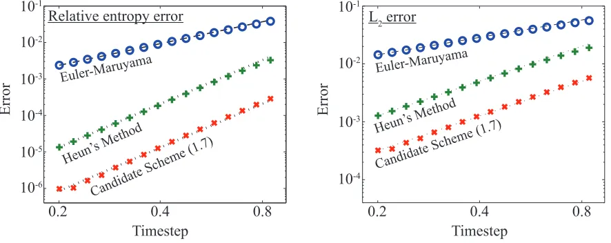
We compute the configurational distribution using each scheme at 16 different timesteps, where the smallest ish= 0.2 and subsequent timesteps are increased by 10%. The distributions are averaged over 32 independent realizations per timestep, and the overall errors are plotted in Figure 1.

0.2

0.4

0.8

10

Timestep

Timestep

L

error

Error

Euler-Maruyama

Heun’s Method

Candidate Scheme (1.7)

10

10

0.2

0.4

0.8

Relative entropy error

Euler-Maruyama

Heun’s Method

Candidate Scheme (1.7)

10

10

10

10

Error

₁₀

10

10

Figure 1: The error in computed distributions is plotted for each scheme at many stepsizes. We compare both the relative entropy (Kullback-Leibler divergence) and theL2 error of the computed distributions ofq. The plotted black guidelines give trends with respect to stepsize, with the dashed and dotted lines giving first and second order respectively in the right plot, and second and fourth order respectively in the left plot.

The results match the analysis given in Section 3 for the large-time regime. In the case of the L2 error, the Euler-Maruyama scheme gives a first order error in the computed distribution, while the other schemes give second order errors. For the computation of relative entropy, we see a doubled rate of convergence (from first to second order, or from second to fourth order). Writing ˆρ=ρ(1 +εψ), whereε

is a small parameter andR

ψρ= 0 (conservation of total probability), we have, Z

ρln[1/(1 +εψ)]dx=−

Z

ρln(1 +εψ)dx=−

Z

ρ(εψ−ε2ψ2+. . .)dx=−ε2Z _ψ2_{ρdx+. . . .}

In the discrete context, if ˆρi=ρi+hkψi for an orderkscheme, then we find that the relative entropy is

proportional toh2k. In practice, we observe that Heun’s method and the method (1.7) give a fourth order relationship with the stepsize, whereas the Euler-Maruyama scheme has relative entropy proportional to

ε2. The non-Markovian method gives approximately an order of magnitude improvement in this example.

5.1.2 Error in finite time

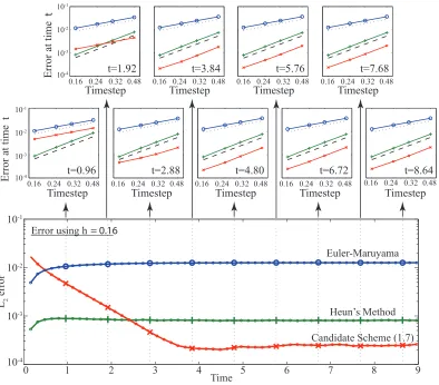
We consider the weak accuracy of the Euler-Maruyama scheme (1.3), Heun’s method (5.1) and the method (1.7). In order to realize the evolving distribution computed for each scheme, we average over 2.56×109 independent trajectories with initial points drawn from a normal distribution with meanπand variance 1 (where the tails of the distribution outside the periodic region are cut off). We divide [0,2π] into 21 histogram bins, and run overt∈[0,9].

L

error

10-1

0.48

0 10-1

2

Euler-Maruyama

Heun’s Method

Candidate Scheme (1.7)

Time Error using h= 0.16

10-2

10-3

10-4

1 2 3 4 5 6 7 8 9

10-4

10-2

10-3

0.16 0.24 0.32 0.48 0.16 0.24 0.32 0.48 0.16 0.24 0.32 0.48 0.16 0.24 0.32 0.48

Timestep Timestep Timestep Timestep

Error at time

t

10-4

10-1

10-2

10-3

0.16 0.24 0.32 0.48 0.16 0.24 0.32 0.48 0.16 0.24 0.32 0.48 0.16 0.24 0.32 0.48 0.16 0.24 0.32

Error at time

t

Timestep Timestep Timestep Timestep Timestep

t=0.96 t=2.88 t=4.80 t=6.72 t=8.64

t=7.68 t=5.76

t=3.84 t=1.92

Figure 2: The lower plot shows the error in the distribution after timet, as computed using each scheme ath= 0.16. In the plots at the top, we compare the error growth with respect to stepsizehat multiples of

t= 0.96. The Euler-Maruyama scheme (◦), Heun’s method (+) and the method (1.7) (×) are compared to first order (dotted) and second order (dashed) guidelines.

and 0.48. The growth of the error at multiples oft= 0.96 is plotted at the top and bottom of Figure 2, along with guidelines to indicate the order of accuracy.

We plot the error after timetfor each scheme, usingh= 0.16, in the central plot of Figure 2. Initially the error in the scheme (1.7) reduces like exp(−λt), but stabilizes aftert= 4. This is due to the behavior described in Section 3, where only the first order component has an exponentially decreasing prefactor. The stabilization occurs when theh2 _{part of the error begins to dominate the observed error.}

5.2

Lennard-Jones box

As a more challenging problem, we compute the error in the radial distribution function forr∈(0,6) for a 6×6×6 periodic box of 64 Lennard-Jones particles, with interaction potential

V(q) = 64 X

i=1 64 X

j=i+1

r_ij−12−r−_ij6, rij=kqi−qjk,

where qi denotes the position of particlei, i.e.,xin (1.1)-(1.2) is 3×64 = 192-dimensional. We chose,

Heun’s Method

Candidate Scheme (1.7)

10-1

Timestep

Error in radial distribution function

0.002 0.003 0.0045

Euler-Maruyama

First order line

Second order line

100

101

102

103

Second order line

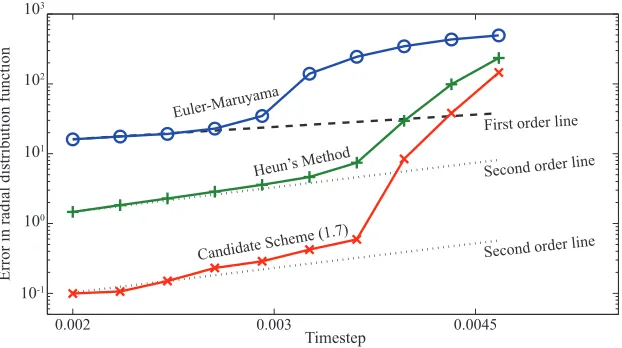
Figure 3: We plot the observedL2error in the computed radial distribution functions for a periodic box of 64 Lennard-Jones particles. The Euler-Maruyama (◦) and the method (1.7) (×) schemes require one force evaluation per step, while Heun’s method (+) requires two.

We observe that the Lipschitz condition (3.1) is not, formally, satisfied for many molecular dynamics potentials (including Lennard-Jones potentials) due to the presence of singularities. Nonetheless it is likely that, due to energetic considerations it would be possible to create a modified domain (a) in which typical solutions remain and (b) in which the Lipschitz condition (3.1) can be verified. The numerical example presented here strongly suggests that the global Lipschitz condition could be relaxed. More directly, the assumption (3.1) can be verified if the potential is replaced by one without singularities, e.g. by using instead Morse potentials, or by a smoothly truncated singular potential, or by a smooth Gaussian approximation of the singular potential [21].

Due to the size and complexity of the problem, we cannot use standard numerical solvers to compute the exact solution. Therefore we compute a baseline solution using the scheme (1.7) to compute 368 realizations of a 107 _{step trajectory (after a 10}6 _{step equilibration period), with a small stepsize of}

h= 0.0016.

We next compute the radial distribution functions computed using the three schemes in Section 5.1, at ten different timesteps beginning ath= 0.002 and with subsequent timesteps increasing by 10%. The trajectories were all taken over a constant time window of [0,20000], with sampling beginning after a 106 step equilibration.

We plot the error for all three schemes in Figure 3. For both the Euler-Maruyama scheme and Heun’s method we average over 32 realizations for each timestep that we consider. This was sufficient to resolve the error introduced by these discretization methods. However, the scheme (1.7) proved to be sufficiently accurate that further computation was required to discern the leading error term, with the error at each timestep computed using 256 realizations to reduce the sampling error.

The results show good agreement with the theory presented in Section 3. The method (1.7) demon-strates an order of magnitude improvement in the long-time error of averages compared to Heun’s method, while at the same time requiring half the cost (in terms of force evaluations).

6

Summary

in the long term (in the transient region, the other methods may of course be better, depending on the problem).

References

[1] A. Abdulle, G. Vilmart, K. Zygalakis. High order numerical approximation of the invariant measure of ergodic SDEs. MATHICSE Technical Report Nr. 27.2013, EPFL, Lausanne, Switzerland, 2013.

[2] A. Abdulle, G. Vilmart, K. Zygalakis. Long time accuracy of Lie-Trotter splitting methods for Langevin dynamics. Submitted, 2014.

[3] V. Bally, D. Talay. The law of the Euler scheme for stochastic differential equations: I. Convergence rate of the distribution function.Prob. Theory Rel. Fields,104(1996), 43–60.

[4] V. Bally, D. Talay. The law of the Euler scheme for stochastic differential equations: II. Convergence rate of the density.Monte Carlo Methods Applic.,2(1996), 93–128.

[5] A. Einstein. On the movement of small particles suspended in a stationary liquid demanded by the molecular kinetic theory of heat, Ann. Phys.17, 549–560, 1905.

[6] A. Einstein. On the theory of the brownian movement, Ann. Phys. 19, 371–381, 1906.

[7] C. Graham, D. Talay.Stochastic Simulation and Monte Carlo Methods: Mathematical Foundations of Stochastic Simulations. Springer, 2013.

[8] R.Z. Hasminskii. Stochastic Stability of Differential Equations. Sijthoff & Noordhoff, 1980.

[9] P.E. Kloeden, E. Platen. Numerical Solution of Stochastic Differential Equations. Springer, 1992.

[10] S. Kullback, R.A. Leibler. On Information and Sufficiency.Ann. of Math. Statist.,22(1951), 79–86.

[11] B. Leimkuhler, C. Matthews. Rational construction of stochastic numerical methods for molecular sampling. Appl. Math. Res. Express2013(2013), 34–56.

[12] B. Leimkuhler, C. Matthews, G. Stoltz. The computation of averages from equilibrium and nonequi-librium Langevin molecular dynamics. arXiv:1308.5814.

[13] J.C. Mattingly, A.M. Stuart, D.J. Higham. Ergodicity for SDEs and approximations: locally Lips-chitz vector fields and degenerate noise.Stoch. Proc. Appl.,101(2002), 185–232.

[14] J.C. Mattingly, A.M. Stuart, M.V. Tretyakov. Convergence of numerical time-averaging and station-ary measures via Poisson equations. SIAM J. Numer. Anal.48(2010), 552–577.

[15] G.N. Milstein, M.V. Tretyakov.Stochastic Numerics for Mathematical Physics.Springer, 2004.

[16] G.N. Milstein, M.V. Tretyakov. Numerical integration of stochastic differential equations with non-globally Lipschitz coefficients.SIAM J. Numer. Anal. 43 (2005), 1139–1154.

[17] G.N. Milstein, M.V. Tretyakov. Computing ergodic limits for Langevin equations. Phys. D, 229 (2007), 81–95.

[18] D. Talay, L. Tubaro. Expansion of the global error for numerical schemes solving stochastic differ-ential equations.Stoch.Anal.Appl.8(1990), 483–509.

[19] D. Talay. Second-order discretization schemes for stochastic differential systems for the computation of the invariant law.Stochastics and Stochastics Reports,29 (1990), 13–36.

[20] G. Vilmart. Postprocessed integrators for the high order integration of ergodic SDEs. Submitted, 2014.