ISSN Online: 2327-4379 ISSN Print: 2327-4352
DOI: 10.4236/jamp.2019.711198 Nov. 27, 2019 2891 Journal of Applied Mathematics and Physics
Four Algorithms for Boundary Control with
Breaking in Space and Time
Vladimir Arabadzhi
Division of Geophysical Research, Institute of Applied Physics, Nizhny Novgorod, Russian
Abstract
Typically, active control systems either have a priori complete information about the boundary-value problem and damped waves before switching on, or get it during the measurement process or accumulate and update informa-tion online (identificainforma-tion process in adaptive systems). In this case, the boundary problem is completely imprinted in the information arrays of the control system. However, very often complete information about a boun-dary-value problem is not available in principle or this info is changing in time faster than the process of its accumulation. The article considers exam-ples of boundary control algorithms based almost without any information. The algorithms presented in the article cannot be obtained within the frame-work of the harmonic representation of the problem by complex amplitudes. And these algorithms carry out fast control in microstructured boundary problems. It is shown that in some cases it is possible to find simple solutions if we remove restrictions: 1) on the spatio-temporal resolution of controlling elements of a boundary-value problem; 2) on the high-frequency radiation of the controlled boundary.
Keywords
Incident Low Frequency Wave, High Frequency Technological Radiation, Fast Control in Microstructured Boundary Problems, Binary Breaker, Breaker-Inverter, Length of Damping, Spinning Acoustic Blades, Gas Stream, Seiche Waves
1. Introduction
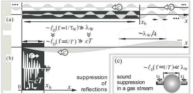
With constant (in time) parameters (or without frequency conversion) devices for wideband non-resonant sound suppression (or other types of waves) should have large wave sizes (thickness D, see Figure 1(a)) of the order of the
maxi-How to cite this paper: Arabadzhi, V. (2019) Four Algorithms for Boundary Control with Breaking in Space and Time. Journal of Applied Mathematics and Phys-ics, 7, 2891-2901.
https://doi.org/10.4236/jamp.2019.711198
DOI: 10.4236/jamp.2019.711198 2892 Journal of Applied Mathematics and Physics mum wavelength λW of the frequency range of suppression λmin <λW<λmax (where λmin/λmax<<1) i.e. D ≥λmax. The goal of this work is to reduce the dimensions of broadband (non-resonant) suppression devices (for cancellation, damping, absorption, suppression of reflections, …) at minimum information on the boundary problem and on the wave to be damped. If we allow the arbi-trary power of high-frequency sound radiation (technological radiation on the technological frequencies f 1/≥ T) and a rapid (on time scale T) change of pa-rameters of a boundary value problem, then in several cases the goals set above can be achieved jointly. Below we will consider some simple applications of this approach. The examples of boundary control considered in the one-dimensional wave problem considered below are reduced to the alternation (in time) of two different types of the boundary-value problem. Jumping (switching) from one boundary-value problem to another and the connection between them provides a certain “breaker” controlled by the algorithm.
We mean breaking as a very quick and microscopic hop (jump) from one boundary value problem to another. Below we want to obtain: (a) effective sup-pression of long wave reflections (Figure 1(a), Figure 1(b)) from a controlled boundary x x= b (and suppression of sound propagation in a gas stream too (Section 5), see Figure 1(c)); (b) in a wide band λmin<<λmax of wavelengths; (c) without accumulation of information about the damped wave and the boundary value problem; (d) at small wave sizes of the suppressing device, i.e. D<<λmin, due to relaxation (dissipation) of the technological waves on high frequencies
f 1/≥ T (i.e. D =D(f)=D(1/ )T ) is length of damping.
2. Algorithm of Half-Return of the Boundary (AHRB)
[image:2.595.218.531.489.641.2]The goal of the algorithm is to suppress reflections from boundary xb. We con-sider a semi-infinite (xb≤ < ∞x ) elastic rod, with longitudinal impedance Z,
DOI: 10.4236/jamp.2019.711198 2893 Journal of Applied Mathematics and Physics sound speed c of waves and the field U x t( , ) of longitudinal displacement of particles (Figure 2(a)). The boundary condition at the end xb has the form
b b
( )[εS U x t∂ ( , ) / ]∂xx x= =F t( ), where F tb( ) is the force applied to end xb, S is the cross-section of the rod, ε is Young’s modulus. A smooth incident wave
W
( , ) ( )
U x t =U x ct+ (temporal scale τW) runs from the right. On the free end
b
x (at Fb =0) we have U tb( ) 2= U x ctW( b+ ) and
/ b( ) b( ) 2 [ W( b )]t
U t U t− −τ ≈ τU x +ct for any interval τ <<τW.
The boundary-value problem can be represented as the sum of two partial li-near problems: (a1) reflection of the incident wave (IW) UW≠0 from the free (at Fb =0) the end of the rod; (a2) wave generation by force Fb ≠0 in the ab-sence of an incident wave (at UW=0). The “breaker” jumps ((a1) ↔ (a2)) in accordance with the control algorithm: measurement in (a1), action in (a2). We assume that the force Fb has a compact support: Fb >0 at t∈[0, ]τF ,
b 0
F = at t∉[0, ]τF . For a clear distinction between the causes and conse-quences in the work of AHRB, it is extremely important that after the termina-tion of the force Fb (at t>τF), the displacement
F 1 b 0 Z F ( )d τ
ξ ξ
−∫
of theboundary xbcaused by this force is saved indefinitely long [1]after its switching off. Now we will directly consider AHRB, which is a sequence of time cycles (see Figure 2(c)) of the boundary control. Each n-th cycle tn 1− ≤ <t tn 1− +Tn of du-ration Tn (n 0,1,2,...= ) consists of two parts: (a) smooth displacement of the free (i.e. at Fb =0) end xb over a time interval tn 1− ≤ <t tn 1− +( )τf n, we set the duration ( )τf n of this interval arbitrary under condition ( )τf n <<τW, and we measure the corresponding displacement [ (U tb n 1− +( ) )τf n −U tb n 1( −)] of boundary xb; (b) the rapid return of the border xb during the interval
n 1 ( )f n n 1 ( )f n ( )r n
t − + τ ≤ <t t− + τ + τ under the action of force Fb. Force F tb( ) is switched off at the moment t t= n 1− +( )τf n+( )τr n when the level
b n 1 f n b n 1 [ (U t − ( ) )τ U t( − )] / 2
− + − becomes crossed by function
n 1 f n n 1 f n
( ) 1 b ( )
[ ] tt ττ ξZ F( )d
ϕ ξ − η η
−
+ + −
+
=
∫
for the first time (at the value ξ=( )τr n) beginningfrom the moment t t= n 1− +( )τf n. It is easy to see from the Figure 2(c) than when the scale T of control cycle, scale τf (( ) ~τf n τf) of free drift, scale τr (( ) ~τr n τr ) of half-return, scale τW of IW are satisfying the condition
r f W
[image:3.595.216.531.587.693.2]τ <<τ <<τ , we get the weakness of reflections on the frequencies f ~ 1/τW or U tb( )→U x ctW( b+ ) and U t U xb( )− W( b+ct U) / W →0, where
DOI: 10.4236/jamp.2019.711198 2894 Journal of Applied Mathematics and Physics W
W (1/ W ) 0 W( ) c
U =
τ
c∫
τ Uξ
dξ
. The peak Pˆhf and average Phf (on the cycle ~T) power of the high-frequency radiation, generated by the impact force Fb, and time averaged power flux PW in the low frequency IW are satisfying to thefol-lowing relations 2
hf W f r
ˆ / ( / ) 1
P P ≈ τ τ >> and P Phf / W ≈τ τf / r >>1. About impedance: Z is unknown and can slowly change in time Z t( ). About impact force: F tb( ) can be of arbitrary pulse shape, but with constant sign and at any moment of impact satisfies the condition Fb>> ΨW, where
W b (1/ W) 0 b( )
F =
τ
∫
τ F t dt, 1 W /W ( / W) 0 ( W( ))
c
x
S τ U x сt dx
ε τ
−Ψ =
∫
+ . About linearity:the returning path scale is h=( /
τ τ
f W)UW, velocity scale is h/τr, so the condi-tion h/τ <<r c ensures linearity.3. Algorithm of Maximum Instant Power Absorbed (AMIP)
The goal of the algorithm AMIP is to maximize the instantaneous power ab-sorbed by the boundary xb. Consider above rod problem: some electric drive (as above “breaker”) can ensure any constant velocity Vb of edge xb inde-pendently of any incident wave (IW). Wave problem can be represented as the sum of two linear problems: (a1) reflection of IW from a fixed (Vb =dU dtb/ =0) boundary xb; (a2) the radiation of waves by a boundary xb at a given velocityb
V in the absence of IW. The breaker jumps: (a1) ↔ (a2). Velocity Vb takes discrete levels V tb n( )=Vn at discrete time intervals (n 1)− T t< <nT (n 1,2,...= ), where T is the period of velocity switching (and measuring between switching). Steps Vn are multiples of the tuning step V, V Vn/ = ± ± ±0, 1, 2, 3,... (integer).
Absorbed power (work of IW with a border xb) is square function
b W b b
( ) ( )[2 ( ) ( )]
W t =V t E x ct ZV t+ − of V t( ) with the unique maximum at
b( ) W( b ) W( b ) /
V t =V x ct+ =E x ct Z+ , where Z=ReZ , V xW( b+ct) and
W( b )
E x ct+ are longitudinal particle velocity and stress in IW in infinite rod. AMIP is expressed by the iterative (recurrent) relation Vn =Vn 1− +Vsgn( )W (for n 2≥ with initial condition V1=0, V V1= ), where: W W= n 1− −Wn 2− ,
n 1 n 1 n 1
W− =F V− − , Wn 2− =F Vn 2 n 2− − ; Fn 1− , Fn 2− are measured values of the force applied to boundary xb by the medium of rod from x x≥ b at the moments
n 1
t − −a , tn 2− −a correspondingly ( 0< <<a T ); sgn( )ξ = +1 at ξ >0 , sgn( )ξ = −1 at ξ<0. If at the previous step the velocity increase causes the
de-crease (W<0) of the absorbed power, at the next step the velocity increase will change its sign and will not change it in the opposite case. In above one dimen-sional statement of the problem absorption maximum corresponds to the min-imum of reflection and radiation too. AMIP does not need to know either rod impedance Z and IW. AMIP effectively traces IW if the following conditions are satisfied: V <<max∂UW/∂t , V T/ >>max∂2UW/ ( )∂t 2 or
2 1 WV UW ( )W T V
τ << << τ − , AMIP resembles the algorithm of random search,
DOI: 10.4236/jamp.2019.711198 2895 Journal of Applied Mathematics and Physics also be applied in the problem of IW absorbing in a thin infinite elastic plate (see Figure 3(b)), since in this case the impedance of the plate with respect to a point source of normal velocity is also purely real (Z=ReZ, [1]). Thus, by adjusting the normal velocity V tb( ) of the point rb of application of external force to the maximum instantaneous absorbed power, it is possible to achieve the maximum absorption cross section σ λ= W / 2π for a point source of the normal plate ve-locity at the point rb.
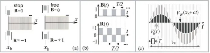
4. Algorithm for Boundary Condition Modulation (ABCM)
The goal of the algorithm is to suppress reflections from boundary xb in the above one-dimensional problem and in layer (or distance from xb) of small thickness at minimum info on IW and boundary problem. The ABCM is based on two main states of a controlled boundary xb (Figure 4(a)): (a1) rigid state [image:5.595.238.496.477.549.2] [image:5.595.193.541.592.680.2]b /
[ ( , )]U x tt x x= =0 with a fixed boundary xb and velocity reflection coefficient 1
= −
R ; (a2) soft state b
/
[ ( , )]U x tx x x= =0 with a free boundary xb and velocity reflection coefficient R= +1. Binary breaker B( )t jumps ((a1) ↔ (a2)) with
period T<<τW and without doing work (without radiation or absorption) and without any measurements. ABCM algorithm controls the boundary condition
b b
/ /
( )[ ( , )]t U x tx x x ( )[ ( , )]t U x tt x x 0
α = +β = = via the coefficients α , β (Figure
4(b)): [B=1,
α
=0, β =1, R= −1] ↔ [B=0,α
=1, β=0, R= +1]. As a result of such control (see Figure 4(c)), we obtain an oscillogram V tb( ) of the velocity of the boundary V tb( ), which on average (over a period T) tends to the velocity of particles in the incident wave (i.e., in an infinite rod without ref-lections) or V tb( )→V x ctW( b+ ) [3], as was required above. An experimental verification of the ABCM algorithm is presented below in Section 6. In this case, the boundary xb converts the low-frequency (with a spatial scale cτW) IWFigure 3. To the algorithm AMIP: boundary velocity and particle velocity in incident wave (a); on the absorption of bending wave in thin infinite elastic plate (b).
DOI: 10.4236/jamp.2019.711198 2896 Journal of Applied Mathematics and Physics wave into reflected high-frequency waves at frequencies f 1/ ,2 / ,3 / ,...= T T T
that dissipatively attenuate in exp[ /− D(f)] times at a distance from the boundary xb, where D=D(f) is the frequency dependent dissipative atten-uation length or equivalent damping device size (see Figure 1(b)).
Thus, having fulfilled the condition cT<<D(1/ )T <<τWc<<D(1/τW), it is possible to ensure the smallness of the attenuation length and smallness of effect of dissipation on the above boundary condition.
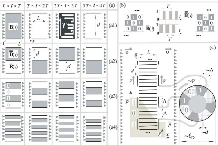
5. Algorithm for Sound Blocking in the Gas Stream (ASBG)
The goal of ASBG is to block the sound propagation in a gas stream with average velocity υ<<c. This problem arises in the design of automobile silencers (Fig-ure 1(c)): we need a device that transmits a gas stream, but does not allow sound propagation in the gas. Traditionally (with parameters constant in time), there are two directions in this problem. On the one hand, pushing of gas through a grid of holes in a rigid plane. The smaller the diameters of the holes, the lower the sound transmission. This approach allows a small size D <<λmin of the si-lencer. But energy losses due to pushing gas through holes increase too much. On the other hand, passing a gas stream with sound through a low pass filter (Helholtz resonator) with resonance at wavelength λ λ> max (with dimensionsD >λmax
). This approach doesn’t require power losses for gas pushing, but re-quires too large dimensions of muffler. Known silencers are usually a combina-tion of approaches (a), (b) or a complicated combinacombina-tion of tubes, perforated plates and resonators. An approach below (based on a quick switching of para-meters) allows dimensions D<<λmin with small power losses for pushing gas through silencer.
DOI: 10.4236/jamp.2019.711198 2897 Journal of Applied Mathematics and Physics Figure 5. On the action of ASBG: (a) temporal sequence of states (“1”—closed state and “0”—opened state) of breakers-inverters at their growing amount ((a1), for 1 waveguide), (a2) 2 waveguides, (a3) 4 waveguides), (a4) 8 waveguides); (b) complementary breakers for the cross section of 3-D problem; (c) running acoustic blades (petals) and spinner.
Next are a lot (Figures 5(a2)-(a4)) of inverters-breakers in the system cross section, now a pair of mutually complementary (B B( ) ( ) 0t t = ) inverter breakers
( )t
B , B( )t (see Figure 5(b)) with the corresponding time diagrams. The more elements in the cross section (Figures 5(a2)-(a4)), the weaker the hydraulic shock (flow energy → sound) when switching inverters and faster this blow becomes blurred (spatially averaged), helping to push the gas into neighboring opened waveguides. The above (evolution in Figure 5(a)) model is difficult to implement (it is not clear how it would be possible to create rapidly appearing and disappearing walls of inverter-breaker). However, the model shown in Fig-ure 5(c) is much simpler to implement. Consider a 2-D echelon of thin infinite parallel rigid plane strips with a length L and with a distance d<<L between them. To the left, a gas flow at time averaged velocity enters this system (and ex-its with the same time averaged velocity υ<<c). Rigid flat thin acoustic blades of width Λ and on distance Λ from each other parallel to the edges of the flat walls at a distance (gap) g<< Λ and run at a speed V <<c. It is easy to verify that each plane waveguide is open during a time interval of duration T and closed (inverter) during the time interval of the same duration T. The condition of synchronism Λ/V L c T= / = . Opening and closing of each waveguide is fulfilled during the time d V/ and very quickly relating to the time of inversion
DOI: 10.4236/jamp.2019.711198 2898 Journal of Applied Mathematics and Physics three-dimensional version of the problem, acoustic blades can be represented by the petals of two spinners rotating in phase near the waveguide bundle (see Fig-ure 5(c)). The spinner doesn’t work with the gas flow (low power for rotation), since its petals are normal to the flow and move parallel to themselves. The dif-ference p p− >0 in the mean (in time and in cross section) gas pressure at the inlet p and outlet p (Figure 5(c)) pushes the gas. Finally we can formulate the following hierarchy of scales for ASBG: λW>>D > >> Λ >> >> >>L d g δ , where λW wavelength of sound in the flow, D-dimension of muffler,
L-length of waveguides, Λ-wideness of blades, d-cross dimension of waveguide,
g-gap between blades and waveguides,
δ
-mean free path of gas molecules. Running blades do not produce high frequency sound (on the frequencies~ /V d ). Above described parametric system equally blocks the propagation of sound from left to right, and from right to left.
6. Experimental Testing of the Algorithm ABCM
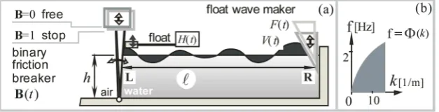
The goal is to reduce the ringingness of a tank (as a resonator for surface water waves) without increasing the viscosity of waveguiding media (water). In the tradi-tional case of time constant parameters (Section 1, Figure 1(a)) of wave-suppressing devices, their dimensions are not less than basin length . The algorithm ABCM (Section 4) was experimentally tested [3] in application to surface water waves in a tank with a length =1.5 m and a filling depth h=0.22 m (see Figure 6(a)). The setup was conceived as an attempt to simulate the above-described one-dimensional boundary acoustic problem for a boundary with a modulated reflection coefficient, despite the two-dimensionality and dis-persion of surface water waves.
6.1. Description of the Experimental Setup
On the left edge of the tank (Figure 6(a)) there is a wall L that can freely ro-tate around an axis located at the bottom. The wall L hermetically (soft corru-gations) separates the water of the tank and the air on the left side.
[image:8.595.218.532.615.695.2]The vertical shift H t( ) of the free surface of the water near the wall L is measured by a sensor in the form of a float. The friction breaker B( )t is switching periodically (with an interval T/ 2 1/ 2f= M, where fM the frequen-cy of binary modulation) between two states: (a) “stopped” state (B( ) 1t = , the breaker strongly pressing to the upper edge L and fixes the angle of deviation
DOI: 10.4236/jamp.2019.711198 2899 Journal of Applied Mathematics and Physics of the wall L); (b) “free” state (B( ) 0t = the breaker does not touch the upper edge L) states of the wall L. Hydrostatic pressure on the wall L on the right is compensated by a soft elastic spring; the softness of spring is such that fre-quency f0 of free (at B( ) 0t = ) oscillations of the wall L is less than the fre-quency of the water wavelength
λ
=2 (seiche). On the right edge of the tank near the vertical rigid wall R there is a weightless (compared to the weight of the displaced water) float, to which the electromagnetic force F t( ) of the wave-generator is applied. The mechanical impedance of the electric drive of the wave maker is negligible compared to the impedance of the mass of water dis-placed by the float. The force F t( ) and speed V t( ) of the vertical displace-ment of the float are measured by appropriate sensors. The dispersion (frequen-cy f [Hz] as a function f = Φ( )k of the wave number k [1/m]) of the propagat-ing waves is shown in Figure 6(b).6.2. Pulse Drive Excitation
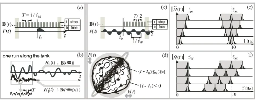
There two experiments with pulsed excitation (Figure 7(a)) were made: 1) exci-tation of the tank (at moment t t= 0) by the pulse of the waveproducing force
( )
F t with the breaker switched off (B( ) 0t = ) and with the registration of damped oscillations H t( )=H t0( ) of the free surface of the water near the wall
L (Figure 7(b)); 2) excitation of the tank (at the moment t t= 0) by the same impulse of the wavemaker force F t( ), but with the breaker switched on (B( ) (0 /1)t = ) and with the recording of damped oscillations H t( )=H t1( ) (Figure 7(b)). As can be seen from Figure 7(b), modulation (B( ) (0 /1)t = ) of the wall L parameters leads to a significant decrease in the wave damping. Since the waves in the tank have dispersion characteristic f= Φ( )k of propa-gating waves, the time of one run of wave along the tank (Figure 6(a)) is esti-mated using the maximum group velocity cg=(2 )[π dΦ/ k]d of the waves as
g max / [ ]c =0.65
s according to the graph presented in Figure 6(b), where
g max
[ ]c ≈1.88 m/s (i.e. at k=0).
6.3. Sinusoidal Excitation of the Tank
The wavemaker on the right wall R (Figure 7(c)) turns on at the moment 0
t= and produces a sinusoidal force F t( ) (at a frequency fW), which is ap-plied to the float, and the breaker B( )t remains off (B( ) 0t = , the wall L is free). By the moment t t= >>0 1/ fW the stationary field of standing waves at a frequency fW is set in the tank and corresponds to a circular trajectory
DOI: 10.4236/jamp.2019.711198 2900 Journal of Applied Mathematics and Physics Figure 7. Pulse excitation ((a), (b)) of the tank: oscillations of the float near the left wall, when the modulation is off, oscillations of the same float when the modulation is switched on. Experiment with sinusoidal excitation of the tank (c). Evolution of the phase trajectory after breaker switching on (d). Scanning of the wavemaker frequency at a constant modulation frequency (e). Scanning of the modulation frequency at a constant wave-maker frequency (f).
high-frequency waves at combination frequencies fM±fW, fM±2fW, … Tra-jectory [ ( ), ( )]F t V t evolutes into a straight line. This means that the wall L represents, from the point of view of the wavemaker, a purely active load ab-sorbing the waves it produces. The fact of the frequency conversion of the wave field by a parametric wall L is clearly illustrated by measurements of the mod-ulus H(f) of the Fourier spectrum H(f) of the oscillations H t( ) of the height of the float near the wall L. Figure 7(e) shows the value H(f) in the case of scanning the frequency fW of the wavemaker, and Figure 7(f) presents the case of scanning the modulation frequency fM. At ideal modulation of the wall L reflection coefficient (R( )t ≈ ±1), there should be no components of the spectrum H(f) at the modulation frequency fM.
7. Conclusion
The algorithms described in the article are constructed for the temporal repre-sentation of a boundary value problem. The presented algorithms are based on the use of high spatial-temporal resolution for fast switching wave regimes and don’t require the accumulation of information about wave fields and the boun-dary problem, using either only instantaneous field measurements or without them. The payment for smallness of information on the fields to be damped and the boundary problem in algorithm is high-frequency radiation. Above breaking algorithms cannot be reduced to either continuous representations (partial dif-ferential equations) or traditional discrete ones (point-like wise in space or (and) in time).
Conflicts of Interest
DOI: 10.4236/jamp.2019.711198 2901 Journal of Applied Mathematics and Physics
References
[1] Budak, B.M., Samarskii, A.A. and Tikhonov, A.N. (1964) A Collection of Problems on Mathematical Physics. Sneddon, I.N., Stark, M. and Ulam, S., Eds., Pergamon, 782p.
[2] Widrow, J.M. and McCool, A. (1976) Comparison of Adaptive Algorithms Based on the Methods of Steepest Descent and Random Search. IEEE Transactions on An-tennas and Propagation, AP-24, 615-637.
https://doi.org/10.1109/TAP.1976.1141414
[3] Arabadzhi, V.V. (2011) Solutions to Problems of Controlling Long Waves with the Help of Micro-Structure Tools. Bentham Science Publishers.