A ‘Non-Parametric’ Version of the Naive Bayes Classifier
Daniele Soriaa,∗, Jonathan M. Garibaldia, Federico Ambrogib, Elia M. Biganzolib, Ian O. Ellisc
aSchool of Computer Science, University of Nottingham, Jubilee Campus, Wollaton Road, Nottingham, NG8 1BB, UK bInstitute of Medical Statistics and Biometry, University of Milan, Via Venezian 1, 20133 Milan, Italy cSchool of Molecular Medical Sciences, Nottingham University Hospitals and University of Nottingham,
Queens Medical Centre, Derby Road, Nottingham, NG7 2UH, UK
Abstract
Many algorithms have been proposed for the machine learning task of classification. One of the simplest
methods, the naive Bayes classifier, has often been found to give good performance despite the fact that its
underlying assumptions (of independence and a Normal distribution of the variables) are perhaps violated.
In previous work, we applied naive Bayes and other standard algorithms to a breast cancer database from
Nottingham City Hospital in which the variables are highly non-Normal and found that the algorithm
performed well when predicting a class that had been derived from the same data. However, when we
then applied naive Bayes to predict an alternative clinical variable, it performed much worse than other
techniques. This motivated us to propose an alternative method, based on naive Bayes, which removes
the requirement for the variables to be Normally distributed, but retains the essential structure and other
underlying assumptions of the method. We tested our novel algorithm on our breast cancer data and on three
UCI datasets which also exhibited strong violations of Normality. We found our algorithm outperformed
naive Bayes in all four cases and outperformed multinomial logistic regression (MLR) in two cases. We
conclude that our method offers a competitive alternative to MLR and naive Bayes when dealing with data
sets in which non-Normal distributions are observed.
Key words: supervised learning, naive Bayes, logistic regression, breast cancer, UCI data sets
1. Introduction
Worldwide, breast cancer is the second most common type of cancer and the fifth most common cause
of cancer death. This disease poses a serious threat for women’s health. Since the early years of cancer
research, biologists have used the traditional microscopic technique to assess tumour behavior for breast
cancer patients. Precise prediction of tumours is critically important for the diagnosis and treatment of
∗Corresponding author. School of Computer Science, University of Nottingham, Jubilee Campus, Wollaton Road,
Notting-ham, NG8 1BB, UK. Tel.: +44 115 95 14229
Email addresses: [email protected](Daniele Soria),[email protected](Jonathan M. Garibaldi),
[email protected](Federico Ambrogi),[email protected](Elia M. Biganzoli),
cancer. Modern machine learning techniques are progressively being used by biologists to obtain proper
tumour information from the databases. Among the existing techniques, supervised learning methods are
the most popular in cancer diagnosis [1].
Many supervised classification algorithms have been proposed in literature, from decision trees to neural
networks, from support vector machines to Bayesian classifiers. The naive Bayes classifier continues to be a
popular learning algorithm for data mining applications due to its simplicity and linear run-time [2]. It is a
fast-supervised classification technique which is suitable for large-scale prediction and classification tasks on
complex and incomplete data sets. Naive Bayesian classification assumes that the variables are independent
given the classes. The naive Bayes classifier applies to learning tasks where each instance x is described
by a conjunction of attribute values and where the target function f(x) can take on any value from same
finite setV [3]. This classifier is based on another common simplifying assumption: the values of numeric
attributes are normally distributed within each class. On many real-world data sets, as in those presented
in this paper, the latter condition is strongly violated. It might happen that, even in such a situation, the
naive Bayes classifier performs well, but one should always be aware that not all the hypotheses are satisfied.
According to John and Langley [4], methods for inducing probabilistic descriptions from training data
have emerged as a major alternative to more established approaches to machine learning, such as
decision-tree induction and neural networks. However, some of the most impressive results to date have come
from a much simpler – and much older – approach to probabilistic induction such as the naive Bayesian
classifier [4]. Despite the simplifying assumptions that underlie the naive Bayesian classifier, experiments
on real-world data have repeatedly shown it to be competitive with much more sophisticated induction
algorithms. Furthermore, naive Bayes can deal with a large number of variables and large data sets, and it
handles both discrete and continuous attribute variables. In [4] the assumption that data are generated by a
single Gaussian distribution is abandoned because it is not always the best approximation. Authors suggest
to investigate more general methods for density estimation, introducing what they call “Flexible Bayes”, an
extension of the naive Bayes classifier which uses a kernel density estimation. This method is very similar
to the naive Bayes, but the density of each continuous variable is estimated averaging over a large set of
kernels. The method performs well in domains that violated the normality assumption and, in general, this
flexible Bayesian classifier generalizes better than the version that assumes a single Gaussian.
Bouckaert [5] also assesses that naive Bayes classifiers perform well over a wide range of classification
problems, and, compared with more sophisticated schemes, they often perform better. He proposes a
comparison of the three main methods for dealing with continuous variables in naive Bayes classifiers, namely
the normal method, the kernel method and discretization. The normal method is the classical method that
approximates the distribution of the continuous variable using a Gaussian distribution. The kernel method
is the one cited above [4] which uses a non-parametric approximation. Finally, the discretization method [6]
variable. In general, it is acknowledged that the normal method tends to perform worse than the other two
methods. However, according to the simulations and experiments run by Bouckaert, none of the three
methods systematically outperforms the others on all problems that were considered.
Much recent work has focussed on the accuracy of the naive Bayes classifier, proposing new alterations
to the technique to improve its performance. Yager [7] provides an extension of the classifier in a manner
that gives the user more parameters for matching data. In particular, a version of naive Bayes is proposed
which involves a weighted summation of products of probabilities.
Hall [2] states that many enhancements to the basic naive Bayes algorithm have been proposed to
help mitigate its primary weakness - the assumption that attributes are independent given the class. He
proposes a simple filter method for setting attribute weights to improve its performance without degrading
the quality of the model. He also considered training time, in that normal naive Bayes algorithm is linear in
both the number of instances and attributes, and his proposed method is supposed to maintain the run-time
complexity and the simplicity of the final model.
According to Lee [8], a different approach to improve the performance of the naive Bayes is to include
unlabeled data as part of the training data in certain problems. Most classic methods of learning with
unlabeled data use a generative model for the classifier and use an Expectation-Maximisation method [9].
Lee’s approach first calculates the estimates of parameters using only labeled data. After acquiring estimated
values of parameters, the algorithm classifies unlabeled data. After the class values of each unlabeled data
are calculated, the algorithm is trained again using both originally labeled data and formerly unlabeled
data. The algorithm iterates this process until there is no or very little change in the estimated target values
of the unlabeled data [8]. Hsu et al. [10] examine the problem of mixed data, stating that the naive Bayes
method is inapplicable when dealing with such data. They propose to use the Extended Naive Bayes and
demonstrate its efficiency in comparison with other classification algorithms.
Many actual data sets are often incomplete for various reasons but most of the supervised learning
techniques deal with complete data. According to Chen and colleagues [11] methods of constructing classifiers
for incomplete data deserve more attention. Classifiers such as naive Bayes classifiers and C4.5 often adopt
two simple strategies to deal with incomplete data: to ignore the instances with unknown entries or to ascribe
these unknown entries to a specified dummy value of the respective attribute variables. To overcome these
limitations, a selective Robust Bayes Classifier for incomplete data based on gain ratio was proposed [11].
The method needs no assumption about the missing data mechanism and, when tested over 12 benchmark
incomplete data sets, showed an improvement in the accuracy of classification with respect to the normal
naive Bayes.
More recently, Balamurugan et al. proposed a method to handle the situation where there is an equal
probability for the class label value, i.e. when the training data satisfy the constraint that the probability of
the naive Bayes classifier fails to classify the record correctly due to the random assignment of class labels.
The approach proposed has been named ‘NB+’, and it aims to suggest a solution with the help of a partial
matching method. The validation of NB+ over 18 public data sets chosen from the UCI machine learning
repository [13] shows a higher degree of accuracy than the traditional naive Bayes algorithm.
Despite the number of approaches proposed for improving the naive Bayes performance, it seems that
a specific criterion for handling non-Normal, continuous and complete data has not been suggested yet. In
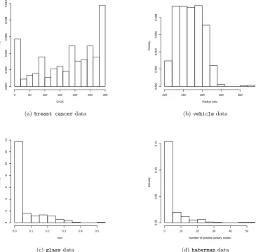
this paper, we present a new method for the implementation of a Bayesian classifier dealing with continuous
variables which, as in our cases, do not follow Normal distributions (see Fig. 1). The motivation for this
new algorithm comes from a previous study [14], in which we reviewed three different supervised learning
techniques and found that the naive Bayes gave the most reliable results although variables were not following
a Normal distribution. In our breast cancer dataset, the variables have distributions that are very far from
Normal and, further, there is no obvious way in which they could be transformed to Normal. Our approach
has the same structure as the naive Bayes one, considering the ratio between areas under the variables’
distribution curves. We compare our new method with both the original naive Bayes algorithm and a
multinomial Logistic Regression model. We aim to show that the new ‘non-parametric’ classifier outperforms
the other two methods or at least is more accurate than the traditional naive Bayes. For our analysis, a
novel dataset on breast cancer [15] and three case series from the UCI Machine Learning Repository [16, 13]
were considered.
[Figure 1 about here.]
The paper is structured as follows. In Section 2, a review of the naive Bayes classifier and its relation
with Logistic Regression are reported. Section 3 describes our new method. Then, in Section 4, the data sets
used for our experiments are presented together with measures for assessing and predicting the accuracy.
Results obtained by the different classifiers are shown in Section 5. Sections 6 and 7, respectively, highlight
the main contributions of this work and discuss the results.
2. Existing Methods
2.1. Naive Bayes Classifier
A naive Bayes classifier is a simple probabilistic classifier based on applying Bayes’ theorem with strong
independence assumptions. LetCbe the random variable denoting the class of an instance andXbe a vector
of random variables denoting the observed attribute values. Letcbe a particular class label andxrepresent
a particular observed attribute value. According to the independence assumption, attributesX1. . . Xn are
all conditionally independent of one another, givenC. The value of this assumption is that it dramatically
the training data [17]. In fact, accurately estimating P(X|C) typically requires many examples. To see
why, let us consider the number of parameters we must estimate whenC is boolean andX is a vector ofn
boolean attributes. In this case, the following set of parameters should be estimated:
θij ≡P(X =xi|C=cj)
where the indexitakes on 2n possible values (one for each of the possible vector values ofX), andjtakes on
2 possible values. Therefore, approximately 2n+1 parameters need to be estimated. To calculate the exact
number of required parameters, note for any fixedj, the sum overi ofθij must be one. Therefore, for any
particular valuecj, and the 2n possible values ofxi, we need compute only 2n−1 independent parameters.
Given the two possible values forC we must estimate a total of 2(2n−1) suchθ
ij parameters for learning
Bayesian classifiers [17]. The Naive Bayes classifier, instead, reduces this complexity by making a conditional
independence assumption that reduces the number of parameters to be estimated, when modelingP(X|C),
form the original 2(2n−1) to just 2n. Moreover, to estimateP(C|X), the training data can be used to learn
estimates ofP(X|C) and P(C). New X examples can then be classified using these estimated probability
distributions, plus Bayes rule. This type of classifier is called agenerativeclassifier, because the distribution
P(X|C) can be viewed as describing how to generate random instancesXconditioned on the target attribute
C[17].
If we have a test casexto classify, the probability of each class given the vector of observed values for
the predictive attributes may be obtained using the Bayes’ theorem:
p(C=c|X =x) = p(C=c)p(X =x|C=c)
p(X =x)
and then predicting the most probable class. Because the event is a conjunction of attribute values
assign-ments, and because of the attributes conditional independence assumption, the following equation may be
written:
p(X =x|C=c) =Y
i
p(Xi=xi|C=c)
which is quite simple to calculate for training and test data [4].
A standard assumption is that, within each class, the values of numeric attributes are normally
dis-tributed. One can represent such a distribution in terms of its mean and standard deviation, and the
probability of an observed value from such estimates can be computed. For continuous attributes we can
write the probability density function for a normal (or Gaussian) distribution as [4]
g(x;µ, σ) =√1
2πσe
−(x−µ)2
2σ2 . (1)
The traditional naive Bayes classifier is still widely used as a popular learning algorithm for data mining
represented by data which often do not satisfy all the assumptions of this technique. To overcome the
non-independence of variables given the class, many techniques have been developed in the past [18]. In this
paper, we are interested in developing a new algorithm which reflects the structure of the naive Bayes, but
that is also able to handle continuous and non-normal data. Solutions like the one proposed by Hsu and
colleagues [10], for example, are then not suitable for our problem, because we are not interested in dealing
with mixed data sets.
2.2. Logistic Regression
Logistic Regression is an approach to learning functions of the formf :X →C, orP(C|X) in the case
whereCis discrete-valued, andX=hX1. . . Xniis any vector containing discrete or continuous variables [17].
Logistic Regression assumes a parametric form for the distribution P(C|X), then directly estimates its
parameters from the training data. In this way, the ‘two-steps’ approach for estimating P(C|X) used by
the naive Bayes may be overtaken. In this sense, Logistic Regression is often referred to as adiscriminative
classifier, because we can view the distribution P(C|X) as directly discriminating the value of the target
C for any given instance X. As shown in [17], if C is boolean and the Gaussian Naive Bayes (GNB)
assumptions hold, then asymptotically (as the number of training examples grows toward infinity) the GNB
and Logistic Regression converge toward identical classifiers. However, as demonstrated in detail in [19],
GNB parameter estimates converge toward their asymptotic values in order lognexamples, wherenis the
dimension ofX. In contrast, Logistic Regression parameter estimates converge more slowly, requiring order
nexamples.
When the response variableCis boolean (0 or 1), the Logistic Regression, fitted by a generalised linear
model (GLM), may be used to model P(1|X); a multinomial logistic regression (MLR) model is instead
needed when there are more than two classes.
3. A ‘Non-Parametric’ Bayesian Classifier
In a previous study [14], three different classification techniques (C4.5 decision tree classifier, Multi-Layer
Perceptron artificial neural network and the naive Bayes classifier) were reviewed and it was found that the
naive Bayes gave the most reliable results even though its simplifying assumptions were strongly violated by
the data analysed. We then thought of developing a new algorithm with the same ‘structure’ of the naive
Bayes, but that could be used with numerical non-normal data. Like the traditional naive Bayesian classifier,
the new algorithm should be a ‘white-box’ model, in which the reason for arriving at the classification can be
explicitly determined by examining the model itself. We were then not interested in using Neural Networks
or Support Vector Machines to replace the naive Bayes because the former are ‘black-box’ models, while the
The main idea of our new algorithm is that the closer a variable value is to its median in a particular
class, the higher is the probability to be assigned to that specific group. This is similar to the traditional
naive Bayes, where the mean is used instead of the median.
At the beginning of the algorithm we computed the median value of each feature in every class and the
priors probabilities, which were defined as the ratio between each class size (in terms of number of data
points) and the total number of cases.
The following step is the main part of our method in which the single probabilities are calculated.
For each variable, we check whether the single variables’ values are smaller or bigger than the median of
that variable distribution in each class. If the value is smaller, we calculate the area under the histogram
which remains on the left with respect to the value being analysed (Fig. 2A). If the amount is bigger, the
area on the right side is computed, taking in consideration the portion of the histogram delimited by the
value and the maximum (Fig. 2B). The amount returned is then divided by half of the total observations,
as we assume that the total area under the histogram is equal to one.
[Figure 2 about here.]
In the next step, for each patient and each class, we compute the product of all the features probabilities
times thepriors.
p[i, k] =priors[k]×
p
Y
j=1
prob[j, k] fork= 1, . . . , K
wherej runs over thepvariables,irepresents patients andK is the number of groups.
The final step of our algorithm is the calculation of the prediction for each instance: it is defined as the
class number which gives the highestp[i, k] (arg maxkp[i, k]).
With a little abuse of notation, we can summarise our algorithm in the following way: calling m, min
and maxthe median, minimum and maximum values of each feature in each class, we want to findk for
whichp[i, k] is maximised, where
p[i, k] =priors[k]×
Y j 1 N/2 Z x min
g(x;m) x < m
Y j 1 N/2 Z max x
g(x;m) x > m ,
1 x=m
andj represents one of the features,xis the particular variable’s value under investigation andiruns over
the instances set. For similarity with the naive Bayes (see Equation 1), we call g(x, m) the function that
represents each variable distribution, even though it is not always possible to express it in an explicit form.
4. Experimental Settings
For our experiments, the WEKA software [20] was used to run the naive Bayes classifier. It is a popular
suite of machine learning free software written in Java and developed at the University of Waikato in
New Zealand. Logistic regression and our new method were run using R, a free software environment for
statistical computing and graphics [21]. All the classification techniques require a reasonable computational
time, especially if compared with neural networks or SVMs [22]. In particular, for the traditional naive
Bayes and for our ‘non-parametric’ Bayesian classifier, the training time is linear in both the number of
instances and attributes [2].
In the next two subsections, the data sets analysed in this study are presented.
4.1. The Nottingham Breast Cancer Data Set
In a previous study [15], immunohistochemistry techniques applied to tissue microarray (TMA)
prepa-rations of 1,076 cases of invasive breast cancer were used to study the combined protein expression profiles
of a large panel of 25 well-characterized biomarkers (reported in Table II of [15]) related to epithelial cell
lineage, differentiation, hormone and growth factor receptors and gene products known to be altered in
some forms of breast cancer. Most of the proteins selected have a well-established role in breast
carcino-genesis. In addition, the gene transcripts of these proteins have been reported to be important candidate
discriminator genes in stratifying breast cancer into distinct groups based on previous cDNA microarray
studies [23, 24, 25, 26, 27, 28].
Several clinical information were also available in this data set, including the Nottingham Prognostic
Index (NPI) score and its defining factors (tumour size, grade, and stage of disease). The NPI was defined
in [29] as a prognostic index which may be used to categorise patients affected by breast cancer according
to its value. In particular, the index is calculated according to the following formula:
N P I Score= (0.2×size) +grade+stage
and five different groups may be defined depending on its value (see Table 1). We used the 25 biomarkers
to predict the NPI groups.
[Table 1 about here.]
4.2. UCI Machine Learning Repository Data Sets
The other datasets we used to validate our new method are taken from the UCI machine learning
repository [13]: vehicle, glass,andhaberman.
For the vehicle dataset, the purpose is to classify a given silhouette as one of four types of vehicle,
angles. The original purpose was to find a method of distinguishing 3D objects within a 2D image by
application of an ensemble of shape feature extractors to the 2D silhouettes of the objects. Measures of
shape features extracted from example silhouettes of objects to be discriminated were used to generate a
classification rule tree by means of computer induction. This object recognition strategy was successfully
used to discriminate between silhouettes of model cars, vans and buses viewed from constrained elevation
but all angles of rotation. The features were extracted from the silhouettes by the HIPS (Hierarchical Image
Processing System), which extracts a combination of scale independent features utilising both classical
moments based measures such as scaled variance, skewness and kurtosis about the major/minor axes and
heuristic measures such as hollows, circularity, rectangularity and compactness. Four ‘Corgie’ model vehicles
were used for the experiment: a double decker bus, Cheverolet van, Saab 9000 and an Opel Manta 400. This
particular combination of vehicles was chosen with the expectation that the bus, van and either one of the
cars would be readily distinguishable, but it would be more difficult to distinguish between the cars [16].
The glass dataset is taken from the USA Forensic Science Service and six types of glass, defined in
terms of their oxide content (i.e. Na, Fe, K, etc), are considered. The study of classification of types of
glass was motivated by criminological investigation: at the scene of the crime, the glass left can be used as
evidence, if it is correctly identified [30, 13].
Thehabermandataset contains cases from study conducted between 1958 and 1970 at the University of
Chicago’s Billings Hospital on the survival of patients who had undergone surgery for breast cancer [31, 13].
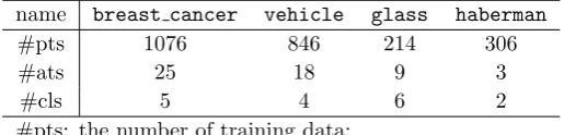
Table 2 provides a summary of thebreast cancerand the three UCI benchmark datasets. Each variable
in each dataset was tested for normality using the Shapiro test [32]. Since no test data sets were provided
in the benchmark sets, we used ten-fold cross validation to evaluate the performance of our algorithm. That
is, each dataset was split randomly into ten subsets and one of those sets was reserved as a test set; this
process was repeated ten times.
[Table 2 about here.]
Since two of the UCI datasets (namely vehicle and glass) had been also analysed by Bouckaert [5],
comparing three main methods for dealing with continuous variables in naive Bayes classifiers, a comparison
with Bouckaert’s results will be performed simply by looking at the average accuracies reported in the
original work [5]. As a matter of fact, in [5], the kernel method and the discretisation one have been used
in comparison with the original naive Bayes.
4.3. Measures for Assessing and Comparing Performance
There are many different measures for predicting the accuracy of a model [33]; two of them arecalibration
anddiscrimination. When a fraction of aboutP of the events we predict with probabilityP actually occur,
been found [34]. Discrimination, instead, measures a predictor’s ability to separate patients with different
responses [33]. When the outcome variable is dichotomous and predictions are stated as probabilities that an
event will occur, calibration and discrimination are more informative than other indices (like, for example,
the expected squared error) in measuring accuracy [33]. Calibration plot is a method that shows how well
the classifier is calibrated and a perfectly calibrated classifier is represented by a diagonal on the graph [35].
In this work, these plots were produced following the procedure described in [34], plotting the fitted values
versus the actual average values.
A c (forconcordance) index is a widely applicable measure of predictive discrimination and it applies
to ordinary continuous outcomes, dichotomous diagnostic outcomes and ordinal outcomes. This index of
predictive discrimination is related to a rank correlation between predicted and observed outcomes. The
c index is defined as the proportion of all usable patient pairs in which the predictions and outcomes are
concordant. For predicting binary outcomes, like in thehabermansurvival dataset,cis identical to the area
under a receiver operating characteristic (ROC) curve [33].
A ROC curve is a tool to measure the quality of a binary classifier independently from the variation in time
of the ratio between positive and negative events [35]. In other words, it is a graphical plot of thesensitivity
versus(1 - specificity)for a binary classifier system as its discrimination threshold is varied. The ROC can
also be represented equivalently by plotting the fraction of true positives (TPR = true positive rate) versus
the fraction of false positives (FPR = false positive rate). A completely random guess would give a point
along a diagonal line (the so-called line of no-discrimination) from the left bottom to the top right corners.
Usually, one is interested in the area under the ROC curve, which gives the probability that a classifier will
rank a randomly chosen positive instance higher than a randomly chosen negative one. A random classifier
has an area of 0.5, while an ideal one has an area of 1.
The accuracies of the obtained classifications were evaluated for all techniques simply by looking at the
percentage of the correctly classified instances.
In the following, the acronyms NB (naive Bayes) and NPBC (non-parametric Bayesian classifier) will
be used to indicate, respectively, the usual naive Bayes classifier and our new method. MLR will stay for
Multinomial Logistic Regression, while GLM for Generalised Linear Model.
5. Experimental Results
First of all, we deleted from the breast cancer data four cases for which the NPI value was missing.
Then, we started our experiments running the naive Bayes classifier in WEKA using the 10-fold cross
validation option. Also when using our new method in R, the 10-fold cross validation option was utilised.
We found, for the breast cancer dataset, that only 249 (23.2%) patients were correctly assigned to
instead, naive Bayes properly classified 381 instances (45.0% of the total amount), leaving 465 cases (55.0%)
incorrectly assigned to their group. When considering theglass dataset, the algorithm correctly classified
almost just half of the cases (48.6% which corresponds to 104 data points), leaving the other half (110 cases,
equal to 51.4%) not properly classified. For the last dataset analysed (haberman), naive Bayes assigned 229
patients (74.8%) to the proper group, and just 77 (25.2%) were misclassified.
With our new algorithm, we found a relevant improvement in the amount of cases that were correctly
classified considering thebreast cancerdataset and more cases were also correctly assigned to their group
when the UCI datasets were analysed. For the breast cancer data, the number of patients which were
assigned to their original class was 416 (38.8%), and 656 (61.2%) were wrongly classified. For thevehicle
data, our method was able to properly classify 503 cases (59.5%), 122 more than with the naive Bayes. The
remaining 343 instances (40.5%) were misclassified even with our new algorithm. When moving to theglass
dataset, we obtained that 121 (56.5%) types were correctly assigned to their group, while the remaining 93
(43.5%) were not. The last dataset considered,haberman, had 240 (78.4%) data points properly classified
and 66 (21.6%) misclassified.
When using a multinomial Logistic Regression model the number of cases correctly classified was higher
with respect to previous techniques for the vehicleand glass data sets, but not for thebreast cancer
one. Concerning the habermandata, for which a GLM was fitted, we got the same results obtained with
the naive Bayes classifier: a total of 229 (74.8%) patients were correctly assigned to their class, while the
remaining 77 (25.2%) were not. A summary of our results is reported in Table 3. For the vehicle and
glass datasets, average accuracies of different naive Bayes methods computed by Bouckaert [5] are also
reported.
[Table 3 about here.]
From Table 3, it can be seen that our new algorithm outperformed the others in two sets of experiments
(breast cancer and haberman data), while in the remaining two the MLR achieved the best accuracy.
However, we were interested in developing an algorithm with a better performance than the traditional
naive Bayes, and this goal was reached in all our tests. Comparisons of our method with black-box models
like Neural Networks were out of the scope of this paper.
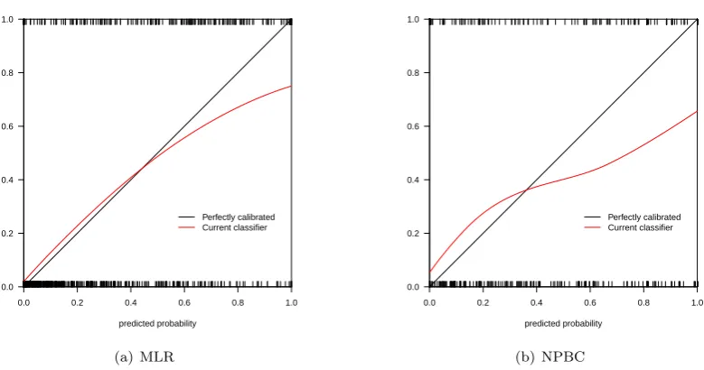
Calibration plots for thebreast cancer,vehicleandglassdata sets are reported in Fig. 3, 4, and 5.
It can be seen that for the novel breast cancer dataset, the Logistic Regression model probabilities are
less calibrated than for our new method. For the other data sets considered, Logistic Regression performed
slightly better than our new algorithm.
[Figure 3 about here.]
[Figure 5 about here.]
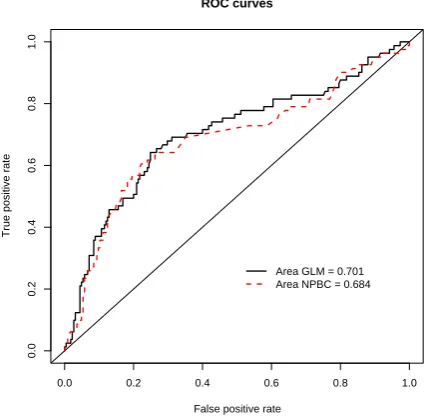
As described in the experiment settings section, for thehabermandata set a plot of the ROC curves for
both the GLM and our method was produced and is reported in Fig. 6. From the values of the areas under
the curves, reported in the plot, a slightly better accuracy of the GLM is evident with respect to our new
method, which, in any case, seems to be a quite good predictive model for thehabermandata.
[Figure 6 about here.]
6. Main contributions
From the results presented in the previous section, two different aspects may be highlighted: firstly, the
new ‘non-parametric’ Bayesian classifier outperforms the traditional naive Bayes for all data sets
consid-ered, showing that the latter classifier is not suitable for problems where variables do not follow a normal
distribution. Moreover, the similarity between our new approach and the naive Bayes one, in terms of
algorithm structure, makes the ‘non-parametric’ method a white-box model. For someone not familiar with
computational analysis it is easier to understand and interpret the set of classification rules derived from a
white-box method.
We should also be aware of some disadvantages of the technique proposed in this work. If used with
normal data, for example, the traditional naive Bayes classifier is likely to be more accurate than our method
(results not shown). In addition, our proposed approach was developed to cope with continuous numerical
data: its validation over mixed data sets remains open for future work.
7. Discussion and Conclusions
In this paper, we reviewed the naive Bayer classifier and applied it to four particular datasets. After
a comparison between the Logistic Regression and the naive Bayes, we presented a new method for the
implementation of a Bayesian classifier which deals with non-normal variables.
Over a novel breast cancer dataset and a set of benchmarks, we applied at the beginning the naive Bayes
classifier, which is based on the assumption that numeric attributes follow a normal distribution. This
method did not perform well on all data considered, and, if we focus on thebreast cancerone, this reflects
a sort of independence between biological markers and clinical information. Moreover, all our datasets’
features strongly violated the normality assumption, thus suggesting that the naive Bayes might not be the
most appropriate method to use.
Supervised learning techniques, like Neural Networks or Support Vector Machines, are widely used for
algorithms for data mining applications due to their linear run-time [2]. However, in many real world
problems, they are not very accurate.
To improve the naive Bayes performance, many different approaches have been proposed in literature [7,
8, 11]. Solutions like the Extended Naive Bayes [10] and the NB+ [12] are only two examples of techniques
being validated over a number of data sets to show a better classification accuracy than the traditional naive
Bayes. However, none of those methods tackled the issue of the non-normality of numerical continuous data.
To solve this problem, we developed an algorithm similar to the naive Bayes but using a ‘non-parametric’
approach.
For each class and each variable, we computed the median value and the histogram of its distribution.
We then considered different situations that might occur: if, fixing a particular class and a particular data
point, the value of a generic variable was lower or greater than the extreme values of the same variable in
the class considered at that stage, then we assigned a probability close to zero to that data point to belong
to the specified class; if the value was identical to the median we set the probability to be one; finally, if the
data point was smaller than the median, we calculated the area between the distribution’s minimum and the
actual value (or between the value and the distribution’s maximum if value was greater than the median).
We then divided the value obtained by half number of observations. As for the naive Bayesian classifier, we
calculated, for each case, the product of probabilities of all features given the classes. We classified our data
looking at the class number for which the above reached the maximum.
With the method just described, we were able to correctly classify a bigger amount of data points with
respect to the naive Bayes, raising the percentage from 23.2% to 38.8% for thebreast cancerdataset, from
45% to almost 60% for the vehicle Statlog dataset, from 48.6% to 56.5% for the glass data, and from
almost 75% to more than 78% for thehabermandataset.
However, when using Logistic Regression, different results were obtained. For the breast cancer
dataset, our model seemed to be more accurate (in terms of percentages of patients correctly classified)
and more calibrated than the Logistic Regression. This was not true when considering the UCI data sets,
for which our algorithm slightly appeared to be less calibrated and less accurate. However, for thehaberman
dataset, when a GLM was fitted to the data, the number of patients correctly assigned to their class was
identical to the one obtained when using naive Bayes and the ROC curve associated to our method was very
similar to the one produced by the GLM, providing two close values for the areas under the curve.
It is important to note that a couple of data sets presented in this work were also used in [5] to compare
naive Bayes normal method with the kernel and the discretization ones obtaining both better and worse
results compared to ours (Table 3). Bouckaert considered those three methods to deal with continuous
variables when using the naive Bayes classifier. Instead our ‘non-parametric’ method was developed to deal
with the non-normality of several dataset variables and, moreover, it outperformed all those proposed in [5]
It is also worth noting that our developed method is not meant to be applicable over all available datasets.
We have showed in this paper several situations for which a classical approach, the naive Bayes classifier,
was outperformed by our more general algorithm that does not assume any particular distribution of the
analysed features.
In conclusion, our proposed technique was more accurate than the traditional naive Bayes in all case
studies analysed, without loosing the characteristics of a white-box model. However, its application over
different types of data has not been investigated yet, leaving space for future research work.
Acknowledgements
This study was supported by the BIOPATTERN FP6 Network of Excellence (FP6-IST-508803) and the
BIOPTRAIN FP6 Marie-Curie EST Fellowship (FP6-007597). Authors would also like to acknowledge the
Turing Institute, Glasgow, Scotland for providing thevehicleStatlog dataset.
References
[1] J. Nahar, Y.-P. Chen, S. Ali, Kernel-based naive bayes classifier for breast cancer prediction, Journal of Biological System
15 (2007) 17–25.
[2] M. Hall, A decision tree-based attribute weighting filter for naive Bayes, Knowledge-Based Systems 20 (2007) 120–126.
[3] T. Mitchell, Machine Learning, McGraw-Hill, 1997.
[4] G. John, P. Langley, Estimating continuous distributions in bayesian classifiers, Proceeding of the Eleventh Conference
on Uncertainty in Artificial Intelligence (1995).
[5] R. Bouckaert, Naive bayes classifiers that perform well with continuous variables, in: Proceedings of the 17th Australian
Conference on AI (AI04), Berlin: Springer, 2004.
[6] J. Dougherty, R. Kohavi, M. Sahami, Supervised and unsupervised discretization of continuous features, in: ICML,
Morgan Kaufmann, 1995, pp. 194–202.
[7] R. Yager, An extension of Naive Bayes classifier, Information Science 176 (2006) 577–588.
[8] C.-H. Lee, Improving classification performance using unlabeled data: Naive Bayesian case, Knowledge-Based Systems
20 (2007) 220–224.
[9] A. Dempster, N. Laird, D. Rubin, Maximum likelihood from incomplete data via the EM algorithm, Journal of the Royal
Statistical Society 39 (1977) 1–38.
[10] C. Hsu, Y. Huang, K. Chang, Extended Naive Bayes classifier for mixed data, Expert Systems with Applications 35
(2008) 1080–1083.
[11] J. Chen, H. Huang, F. Tian, S. Tian, A selective Bayes Classifier for classifying incomplete data based on gain ratio,
Knowledge-Based Systems 21 (2008) 530–534.
[12] A. alias Balamurugan, R. Rajaram, Pramala, Rajalakshmi, Jeyendran, Dinesh, NB+: An improved Naive Bayesian
algorithm, Knowledge-Based Systems In Press, Uncorrected Proof (2010).
[13] A. Asuncion, D. Newman, UCI machine learning repository, http://archive.ics.uci.edu/ml/, 2007. University of California,
Irvine, School of Information and Computer Sciences.
[14] D. Soria, J. Garibaldi, E. Biganzoli, I. Ellis, A comparison of three different methods for classification of breast cancer
[15] D. Abd El-Rehim, G. Ball, S. Pinder, E. Rakha, C. Paish, J. Robertson, D. Macmillan, R. Blamey, I. Ellis,
High-throughput protein expression analysis using tissue microarray technology of a large well-characterised series identifies
biologically distinct classes of breast cancer confirming recent cDNA expression analyses, Int. Journal of Cancer 116
(2005) 340–350.
[16] J. Siebert, Vehicle recognition using rule based methods, Turing Institute Research Memorandum TIRM-87-018 (1987).
[17] T. Mitchell, Generative and discriminative classifiers: Naive bayes and logistic regression, 2005. Freely available at
http://www.cs.cmu.edu/˜tom/mlbook/NBayesLogReg.pdf.
[18] Z. Zheng, G. Webb, Lazy learning of bayesian rules, Machine Learning 41 (2000) 53–84.
[19] A. Ng, M. Jordan, On discriminative vs. generative classifiers: A comparison of logistic regression and naive bayes,
Advances in Neural Information Processing Systems (NIPS) 14 (2002).
[20] I. Witten, E. Frank, Data Mining: Practical Machine Learning Tools and Techniques with Java Implementations, Morgan
Kaufmann, San Francisco, 2000.
[21] J. Maindonald, W. Braun, Data Analysis and Graphics Using R - An Example-Based Approach, Cambridge University
Press, 2003.
[22] L. Xu, M.-Y. Chow, X. Gao, Comparisons of logistic regression and artificial neural network on power distribution systems
fault cause identification, in: 2005 IEEE Mid-Summer Workshop on Soft Computing in Industrial Applications.
[23] C. Perou, T. Sorlie, M. Eisen, M. Van De Rijn, S. Jeffrey, C. Rees, J. Pollack, D. Ross, H. Johnsen, L. Akslen, O. Fluge,
A. Pergamenschikov, C. Williams, S. Zhu, P. Lonning, A. Borresen-Dale, P. Brown, D. Botstein, Molecular portraits of
human breast tumours, Nature 406 (2000) 747–752.
[24] J. Pollack, T. Sorlie, C. Perou, C. Rees, S. Jeffrey, P. Lonning, R. Tibshirani, D. Botstein, A. Borresen-Dale, P. Brown,
Microarray analysis reveals a major direct role of DNA copy number alteration in the transcriptional program of human
breast tumors, Proc Natl Acad Sci U S A 99 (2002) 12963–12968.
[25] T. Sorlie, C. Perou, R. Tibshirani, T. Aas, S. Geisler, H. Johnsen, T. Hastie, M. Eisen, M. Van De Rijn, S. Jeffrey,
T. Thorsen, H. Quist, J. Matese, P. Brown, D. Botstein, P. Eystein Lonning, A. Borresen-Dale, Gene expression patterns
of breast carcinomas distinguish tumor subclasses with clinical implications, Proc Natl Acad Sci U S A 98 (2001) 10869–
10874.
[26] L. Van’T Veer, H. Dai, M. Van De Vijver, Y. He, A. Hart, R. Bernards, S. Friend, Expression profiling predicts outcome
in breast cancer, Breast Cancer Res 5 (2003) 57–58.
[27] M. Van De Vijver, Y. He, L. Van’T Veer, H. Dai, A. Hart, D. Voskuil, G. Schreiber, J. Peterse, C. Roberts, M. Marton,
M. Parrish, D. Atsma, A. Witteveen, A. Glas, L. Delahaye, T. Van Der Velde, H. Bartelink, S. Rodenhuis, E. Rutgers,
S. Friend, R. Bernards, A gene-expression signature as a predictor of survival in breast cancer, N Engl J Med 347 (2002)
1999–2009.
[28] A. Naderi, A. Teschendorff, N. Barbosa-Morais, S. Pinder, A. Green, D. Powe, J. Robertson, S. Aparicio, I. Ellis, J. Brenton,
C. Caldas, A gene-expression signature to predict survival in breast cancer across independent data sets, Oncogene 26
(2006) 1507–1516.
[29] M. Galea, R. Blamey, C. Elston, I. Ellis, The Nottingham Prognostic Index in primary breast cancer, Breast Cancer Res
Treat 22 (1992) 207–219.
[30] I. Evett, E. Spiehler, Rule induction in forensic science, in: KBS in Goverment, Online Publications, 1987, pp. 107–118.
[31] S. Haberman, Generalized residuals for log-linear models, in: Proceedings of the 9th International Biometrics Conference,
pp. 104–122.
[32] P. Royston, Algorithm as 181: The w test for normality, Applied Statistics 31 (1982) 176–180.
[33] F. Harrell Jr., K. Lee, D. Mark, Multivariable prognostic models: Issues in developing models, evaluating assumptions
[34] W. Venables, B. Ripley, Modern Applied Statistics with S, New York: Springer, 4th edition, 2002.
List of Figures
1 Histogram of sample variables . . . 18
2 Area under the histogram . . . 19
3 Calibration plots for multinomial logistic fit to thebreast cancerdata. MLR: Multinomial Logistic Regression, NPBC: Non-Parametric Bayesian Classifier . . . 19
4 Calibration plots for multinomial logistic fit to thevehicledata . . . 20
5 Calibration plots for multinomial logistic fit to theglassdata . . . 20
CK18
Density
0 50 100 150 200 250 300
0.000
0.002
0.004
0.006
0.008
0.010
(a)breast cancerdata
Radius ratio
Density
100 150 200 250 300
0.000
0.002
0.004
0.006
0.008
(b)vehicledata
Iron
Density
0.0 0.1 0.2 0.3 0.4 0.5
0
2
4
6
8
10
12
14
(c)glassdata
Number of positive axillary nodes
Density
0 10 20 30 40 50
0.00
0.05
0.10
0.15
[image:18.595.113.479.133.493.2](d)habermandata
ER
D
en
si
ty
0 50 100 150 200 250 300
0. 000 0. 005 0. 010 0. 01 5 ER D en si ty
0 50 100 150 200 250 300
0. 000 0. 005 0. 010 0. 01 5 m e d ia n da ta po in t
(a) If the value is smaller than the median
ER
D
en
si
ty
0 50 100 150 200 250 300
0. 000 0. 005 0. 010 0. 01 5 ER D en si ty
0 50 100 150 200 250 300
0. 000 0. 005 0. 010 0. 01 5 da ta po in t m ed ia n
[image:19.595.99.508.157.346.2](b) If the value is bigger than the median
Figure 2: Area under the histogram
0.0 0.2 0.4 0.6 0.8 1.0
0.0 0.2 0.4 0.6 0.8 1.0 predicted probability Perfectly calibrated Current classifier (a) MLR
0.0 0.2 0.4 0.6 0.8 1.0
[image:19.595.106.496.458.674.2]0.0 0.2 0.4 0.6 0.8 1.0 predicted probability Perfectly calibrated Current classifier (b) NPBC
0.0 0.2 0.4 0.6 0.8 1.0 0.0
0.2 0.4 0.6 0.8 1.0
predicted probability
Perfectly calibrated Current classifier
(a) MLR
0.0 0.2 0.4 0.6 0.8 1.0
0.0 0.2 0.4 0.6 0.8 1.0
predicted probability
Perfectly calibrated Current classifier
[image:20.595.107.498.159.365.2](b) NPBC
Figure 4: Calibration plots for multinomial logistic fit to thevehicledata
0.0 0.2 0.4 0.6 0.8 1.0
0.0 0.2 0.4 0.6 0.8 1.0
predicted probability
Perfectly calibrated Current classifier
(a) MLR
0.0 0.2 0.4 0.6 0.8 1.0
0.0 0.2 0.4 0.6 0.8 1.0
predicted probability
Perfectly calibrated Current classifier
(b) NPBC
[image:20.595.107.497.474.679.2]ROC curves
False positive rate
True positive rate
0.0 0.2 0.4 0.6 0.8 1.0
0.0
0.2
0.4
0.6
0.8
1.0
[image:21.595.187.401.309.518.2]Area GLM = 0.701 Area NPBC = 0.684
List of Tables
1 NPI groups according to the value . . . 23 2 Summary of the datasets used (‘breast cancer’ plus three from UCI) . . . 23 3 Comparison of results. NB: Naive Bayes; MLR: Multinomial Logistic Regression; BK:
NPI Score Prognostic Group
≤2.4 Excellent Prognostic Group (EPG) 2.5 - 3.4 Good Prognostic Group (GPG) 3.5 - 4.4 Moderate Prognostic Group 1 (MPG1) 4.5 - 5.4 Moderate Prognostic Group 2 (MPG2)
[image:23.595.171.424.110.193.2]>5.4 Poor Prognostic Group (PPG)
Table 1: NPI groups according to the value
name breast cancer vehicle glass haberman
#pts 1076 846 214 306
#ats 25 18 9 3
#cls 5 4 6 2
#pts: the number of training data;
[image:23.595.169.427.313.375.2]#ats: the number of attributes of patterns; #cls: the number of classes.
Table 2: Summary of the datasets used (‘breast cancer’ plus three from UCI)
breast cancer vehicle glass haberman
Method Classified Miscl. Classified Miscl. Classified Miscl. Classified Miscl.
NB 249 (23.2%) 823 381 (45.0%) 465 104 (48.6%) 110 229 (74.8%) 77
MLR 332 (31.0%) 740 678 (80.1%) 168 134 (62.6%) 80 229 (74.8%) 77
BK [5] — — (60.9%) (39.1%) (51.1%) (48.9%) — —
BD [5] — — (61.1%) (38.9%) (71.9%) (28.1%) — —
NPBC 416 (38.8%) 656 503 (59.5%) 343 121 (56.5%) 93 240 (78.4%) 66
[image:23.595.78.519.527.613.2]