Markov switching generalized additive models

DOI 10.1007/s11222-015-9620-3

Markov-switching generalized additive models

Roland Langrock1 · Thomas Kneib2 · Richard Glennie3 · Théo Michelot4

Received: 11 May 2015 / Accepted: 15 December 2015 / Published online: 28 December 2015 © The Author(s) 2015. This article is published with open access at Springerlink.com

Abstract We consider Markov-switching regression mod-els, i.e. models for time series regression analyses where the functional relationship between covariates and response is subject to regime switching controlled by an unobservable Markov chain. Building on the powerful hidden Markov model machinery and the methods for penalized B-splines routinely used in regression analyses, we develop a frame-work for nonparametrically estimating the functional form of the effect of the covariates in such a regression model, assuming an additive structure of the predictor. The result-ing class of Markov-switchresult-ing generalized additive models is immensely flexible, and contains as special cases the com-mon parametric Markov-switching regression models and also generalized additive and generalized linear models. The feasibility of the suggested maximum penalized likelihood approach is demonstrated by simulation. We further illustrate the approach using two real data applications, modelling (i) how sales data depend on advertising spending and (ii) how energy price in Spain depends on the Euro/Dollar exchange rate.

Keywords P-splines·Hidden Markov model·Penalized likelihood·Time series regression

B

[email protected] 1 _{Bielefeld University, Bielefeld, Germany} 2 _{University of Göttingen, Göttingen, Germany} 3 _{University of St Andrews, St Andrews, UK} 4 _{INSA de Rouen, Saint-Étienne-du-Rouvray, France}

1 Introduction

In regression scenarios where the data have a time series structure, there is often parameter instability with respect to time (Kim et al. 2008). A popular strategy to account for such dynamic patterns is to employ regime switching where parameters vary in time, taking on finitely many values, controlled by an unobservable Markov chain. Such mod-els are referred to as Markov-switching or regime-switching regression models, following the seminal papers byGoldfeld

and Quandt(1973) andHamilton(1989). A basic

Markov-switching regression model involves a time series{Yt}t=1,...,T

and an associated sequence of covariatesx1, . . . ,xT

(includ-ing the possibility ofxt = yt₋1), with the relation between

xtandYt specified as

Yt = f(st)(_xt)+σ

stt, (1)

where typicallyt ii d

∼ N(0,1)andst is the state at timet

of an unobservable N-state Markov chain. In other words, the functional form of the relation between xt andYt and the residual variance change over time according to state switches of an underlying Markov chain, i.e. each state corresponds to a regime with different stochastic dynam-ics. The Markov chain induces serial dependence, typically such that the states are persistent in the sense that regimes are active for longer periods of time, on average, than they would be if an independent mixture model was used to select among regimes. The classic example is an economic time series where the effect of an explanatory variable may differ between times of high and low economic growth (Hamilton 2008).

covariates or for general error distributions from the gen-eralized linear model (GLM) framework. An example for the latter is the Markov-switching Poisson regression model discussed in Wang and Puterman (2001). However, in the existing literature the relationship between the target vari-able and the covariates is commonly specified in parametric form and usually assumed to be linear, with little investiga-tion, if any, into the absolute or relative goodness of fit. The aim of the present work is to provide effective and accessible methods for a nonparametric estimation of the functional form of the predictor. These build on a) the strengths of the hidden Markov model (HMM) machinery (Zucchini and MacDonald 2009), in particular the forward algorithm, which allows for a simple and fast evaluation of the likelihood of a Markov-switching regression model (parametric or nonpara-metric), and b) the general advantages of penalized B-splines, i.e. P-splines (Eilers and Marx 1996), which we employ to obtain almost arbitrarily flexible functional estimators of the relationship between target variable and covariate(s). Model fitting is done via numerical maximum penalized like-lihood estimation, using either generalized cross-validation or an information criterion approach to select smoothing parameters that control the balance between goodness-of-fit and smoothness. Since parametric polynomial models are included as limiting cases for very large smoothing parameters, this procedure also comprises the possibility to effectively reduce the functional effects to their para-metric limiting cases, such that the conventional parapara-metric Markov-switching regression models effectively are nested special cases of our more flexible models.

Our approach is by no means limited to models of the form given in (1). In fact, the flexibility of the HMM machin-ery allows for the consideration of models from a much bigger class, which we termMarkov-switching generalized

additive models(MS-GAMs). These are simply generalized

additive models (GAMs) with an additional time component, where the predictor—including additive smooth functions of covariates, parametric terms and error terms—is subject to regime changes controlled by an underlying Markov chain, analogously to (1). While the methods do not necessitate a restriction to additive structures, we believe these to be most relevant in practice and hence have decided to focus on these models in the present work. Our work is closely related to that ofSouza and Heckman(2014). Those authors, however, confine their consideration to the case of only one covariate and the identity link function. Furthermore, we note that our approach is similar in spirit to that proposed inLangrock et al.

(2015), where the aim is to nonparametrically estimate the densities of the state-dependent distributions of an HMM.

The paper is structured as follows. In Sect.2, we formulate general Markov-switching regression models, describe how to efficiently evaluate their likelihood, and develop the spline-based nonparametric estimation of the functional form of the

predictor. The performance of the suggested approach is then investigated in three simulation experiments in Sect.3. In Sect. 4, we demonstrate the feasibility and the potential of the approach by applying it (i) to advertising data and (ii) to Spanish energy price data. We conclude in Sect.5.

2 Markov-switching generalized additive models

2.1 Markov-switching regression models

We begin by formulating a Markov-switching regression model with arbitrary form of the predictor, encompass-ing both parametric and nonparametric specifications. Let

{Yt}t₌1,...,T denote the target variable of interest (a time

series), and let xp1, . . . ,xpT denote the associated values

of the pth covariate considered, where p = 1, . . . ,P. We summarize the covariate values at time t in the vec-torx_·t = (x1t, . . . ,xPt). Further let s1, . . . ,sT denote the

states of an underlying unobservable N-state Markov chain

{St}t=1,...,T. Finally, we assume that conditional on(st,x·t), Ytfollows some distribution from the exponential family and is independent of all other states, covariates and observations. We write

gE(Yt |st,x·t)

=η(st)(_x

·t), (2)

where g is some link function, typically the canonical link function associated with the exponential family distribution considered. That is, the expectation of Yt is linked to the covariate vector x_·t via the predictor function η(i), which

maps the covariate vector toR, when the underlying Markov chain is in statei, i.e.St =i. Essentially there is one regres-sion model for each statei,i =1, . . . ,N. In the following, we use the shorthandμ(st)

t =E(Yt |st,x·t).

To fully specify the conditional distribution ofYt, addi-tional parameters may be required, depending on the error distribution considered. For example, if Yt is condition-ally Poisson distributed, then (2) fully specifies the state-dependent distribution (e.g. withg(μ) = log(μ)), whereas ifYt is normally distributed (in which casegusually is the identity link), then the variance of the error needs to be spec-ified, and would typically be assumed to also depend on the current state of the Markov chain. We use the notationφ(st)_to

denote such additional state-dependent parameters (typically dispersion parameters), and denote the conditional density ofYt, given(st,x_·t), aspY(yt, μ(tst), φ(st)). The simplest and

probably most popular such model assumes a conditional normal distribution forYt, a linear form of the predictor and a state-dependent error variance, leading to the model

Yt =β(st)_+β(st)_x

where t ii d

∼ N(0,1)(cf. Frühwirth-Schnatter 2006; Kim et al. 2008).

Assuming homogeneity of the Markov chain—which can easily be relaxed if desired—we summarize the probabili-ties of transitions between the different states in theN×N

transition probability matrix (t.p.m.) = γi j

, where γi j = Pr

St₊1 = j|St = i

,i,j = 1, . . . ,N. The initial state probabilities are summarized in the row vectorδ, where δi =Pr(S1 =i),i =1, . . . ,N. It is usually convenient to

assumeδto be the stationary distribution, which, if it exists, is the solution toδ=δsubject toiN=1δi =1.

2.2 Likelihood evaluation by forward recursion

A Markov-switching regression model, with conditional density pY(yt, μ(st)

t , φ(st)) and underlying Markov chain

characterized by(,δ), can be regarded as an HMM with additional dependence structure (here in the form of covari-ate influence); see Zucchini and MacDonald (2009). This opens up the way for exploiting the efficient and flexible HMM machinery. Most importantly, irrespective of the type of exponential family distribution considered, an efficient recursion can be applied in order to evaluate the likelihood of a Markov-switching regression model, namely the so-called forward algorithm. To see this, consider the vectors of for-ward variables, defined as the row vectors

αt =

αt(1), . . . , αt(N)

, t =1, . . . ,T,

whereαt(j)=p(y1, . . . ,yt,St = j |x·1. . .x·t)

for j =1, . . . ,N.

Herepis used as a generic symbol for a (joint) density. Then the following recursive scheme can be applied:

α1=δQ(y1) ,

αt =αt−1Q(yt) (t=2, . . . ,T), (4)

where

Q(yt)=diagpY(yt, μt(1), φ(1)), . . . ,pY(yt, μ( N) t , φ(N))

.

The recursion (4) follows immediately from

αt(j)= N

i=1

αt−1(i)γi jpY(yt, μ(tj), φ(j)),

which in turn can be derived in a straightforward manner using the model’s dependence structure. Thus, the forward algorithm exploits the conditional independence assump-tions to perform the likelihood calculation recursively, tra-versing along the time series and updating the likelihood and

state probabilities at every step. The likelihood can then be written as a matrix product:

L(θ)= N

i=1

αT(i)=δQ(y1)Q(y2) . . .Q(yT)1, (5)

where1∈RNis a column vector of ones, and whereθis a vector comprising all model parameters. The computational cost of evaluating (5) is linear in the number of observations,

T, such that a numerical maximization of the likelihood is feasible in most cases, even for very large T and moderate numbers of statesN.

2.3 Nonparametric modelling of the predictor

Notably, the likelihood form given in (5) applies for any form of the conditional densitypY(yt, μ(st)

t , φ(st)). In particular, it

can be used to estimate simple Markov-switching regression models, e.g. with linear predictors, or in fact with any GLM-type structure within states. Here we are concerned with a nonparametric estimation of the functional relationship betweenYt andx_·t. To achieve this, we consider a

GAM-type framework (Wood 2006), with the predictor comprising additive smooth state-dependent functions of the covariates:

g(μ(st)

t )=η(st)(x·t)=β₀(st)+ f₁(st)(x1t)+ f₂(st)(x2t) + · · · + f(st)

P (xPt).

We simply have one GAM associated with each state of the Markov chain. To achieve a flexible estimation of the func-tional form, we use penalised splines as introduced byEilers and Marx(1996) (see alsoFahrmeir et al. 2013, for an in-depth discussion of penalised splines) and express each of the functions fp(i),i =1, . . . ,N,p=1, . . . ,P, as a finite linear

combination of a high number of B-spline basis functions,

B1, . . . ,BK:

fp(i)(x)=

K

k=1

γi pkBk(x). (6)

Note that different sets of basis functions can be applied to represent the different functions, but to keep the notation simple we here consider a common set of basis functions for all fp(i). B-splines have turned out to form a

of basis functions allows for an increasing curvature of the function being modeled. Instead of trying to select an opti-mal number of basis elements, we followEilers and Marx

(1996) and modify the likelihood by including a difference penalty on coefficients of adjacent B-splines. The number of basis B-splines,K, then simply needs to be sufficiently large in order to yield high flexibility for the functional esti-mates. Once this threshold is reached, a further increase in the number of basis elements no longer changes the fit to the data due to the impact of the penalty. Considering second-order differences—which leads to an approximation of the integrated squared curvature of the function estimate

(Eilers and Marx 1996)—leads to the difference penalty

0.5λi pkK=3(2γi pk)2, whereλi p ≥0 are smoothing

para-meters and where2γi pk=γi pk−2γi p,k−1+γi p,k−2. Note

that the integrated squared second derivative could of course also be evaluated explicitly for cubic B-splines. However, the approximation via a difference penalty allows to avoid the associated implementational costs at basically no cost in terms of the fit.

We then modify the (log-)likelihood of the MS-GAM— specified by pY(yt, μ(st)

t , φ(st)) in combination with (6)

and underlying Markov chain characterized by(,δ)—by including the above difference penalty, one for each of the smooth functions appearing in the state-dependent predic-tors:

lpen.(θ)=log

L(θ)− N

i=1

P

p=1

λi p

2

K

k=3

(2_γ

i pk)2. (7)

The maximum penalized likelihood estimate then reflects a compromise between goodness-of-fit and smoothness, where an increase in the smoothing parameters leads to an increased emphasis being put on smoothness. We discuss the choice of the smoothing parameters in more detail in Sect.2.5. Asλi p → ∞, the corresponding penalty

domi-nates the log-likelihood, leading to a sequence of estimated coefficientsγi p1, . . . , γi p K that are on a straight line. Thus,

we obtain the common linear predictors, as given in (3), as a limiting case. Similarly, we can obtain parametric functions with arbitrary polynomial orderq as limiting cases by con-sidering(q+1)th order differences in the penalty. Thus, the common parametric regression models are essentially nested within the class of nonparametric models that we consider. One can of course obtain these nested special cases more directly, by simply specifying parametric rather than non-parametric forms for the predictor. On the other hand, it can clearly be advantageous not to constrain the functional form in any way a priori, though still allowing for the possibility of obtaining constrained parametric cases as a result of a data-driven choice of the smoothing parameters. Standard GAMs and even GLMs are also nested in the considered class of

models (N =1), but this observation is clearly less relevant, since powerful software is already available for these special cases.

2.4 Inference

For given smoothing parameters and given number of states, all model parameters—including the parameters determining the Markov chain, any dispersion parameters, the coeffi-cientsγi pkused in the linear combinations of B-splines and

any other parameters required to specify the predictor—can be estimated simultaneously by numerically maximizing the penalized log-likelihood given in (7). For each function fp(i), i =1, . . . ,N, p =1, . . . ,P, one of the coefficients needs to be fixed to render the model identifiable, such that the intercept controls the height of the predictor function. A con-venient strategy to achieve this is to first standardize each sequence of covariatesxp1, . . . ,xpT, p =1, . . . ,P,

shift-ing all values by the sequence’s mean and dividshift-ing the shifted values by the sequence’s standard deviation, and second con-sider an odd number of B-spline basis functions K with γi p,(K+1)/2=0 fixed.

The numerical maximization is carried out subject to well-known technical issues arising in all optimization problems, including parameter constraints and local maxima of the likelihood. The latter can be either easy to deal with or a chal-lenging problem, depending on the complexity of the model considered. Numerical underflow (or overflow), which would typically arise for largeT if the likelihood itself was consid-ered, is prevented via the consideration of thelog-likelihood. Since the likelihood is a product of matrices, this requires the implementation of a scaling algorithm (for details, see, e.g.,

Zucchini and MacDonald 2009). Any suitable optimization

routine can be applied to perform the likelihood maximiza-tion. In this work, we used R and the optimizernlm, which is a non-linear minimizer based on a Newton-type optimiza-tion routine. For more details on the algorithm, seeSchnabel et al.(1985).

a pre-specified fraction of all bootstrapped curves completely (Krivobokova et al. 2010).

For the closely related class of nonparametric HMMs, identifiability holds under fairly weak conditions, which in practice will usually be satisfied, namely that the t.p.m. of the unobserved Markov chain has full rank and that the state-specific distributions are distinct (Gassiat et al. in press). This result transfers to the more general class of MS-GAMs if, additionally, the state-specific GAMs are identifiable. Con-ditions for the latter are simply the same as in any standard GAM. In particular, the nonparametric functions have to be centered around zero. Furthermore, in order to guarantee estimability of a flexible smooth function on a given domain, it is necessary that the covariate values cover that domain sufficiently well. In practice, i.e. when dealing with finite sample sizes, parameter estimation will be difficult if the level of correlation, as induced by the unobserved Markov chain, is low, and also if the state-specific GAMs are similar. The stronger the correlation in the state process, the clearer becomes the pattern and hence the easier it is for the model to allocate observations to states. Similarly, the estimation performance will be best, in terms of numerical stability, if the state-specific GAMs are clearly distinct. (See also the simulation experiments in Sect.3below.)

2.5 Choice of the smoothing parameters

In Sect. 2.4, we described how to fit an MS-GAM to data for a given smoothing parameter vector. To choose adequate smoothing parameters in a data-driven way, gen-eralized cross-validation can be applied. A leave-one-out cross-validation will typically be computationally infeasi-ble. Instead, for a given time series to be analyzed, we generateC random partitions such that in each partition a high percentage of the observations, e.g. 90 %, form the calibration sample, while the remaining observations con-stitute the validation sample. For each of theC partitions and anyλ=(λ11, . . . , λ1P, . . . , λN1, . . . , λN P), the model

is then calibrated by estimating the parameters using only the calibration sample (treating the data points from the valida-tion sample as missing data, which is straightforward using the HMM forward algorithm; seeZucchini and MacDon-ald 2009). Subsequently, proper scoring rules (Gneiting and Raftery 2007) can be used on the validation sample to assess the model for the givenλand the corresponding calibrated model. For computational convenience, we consider the log-likelihood of the validation sample, under the model fitted in the calibration stage, as the score of interest (now treat-ing the data points from the calibration sample as misstreat-ing data). From some pre-specified grid ⊂ R_≥N₀×P, we then select theλ that yields the highest mean score over theC

cross-validation samples. The number of samplesCneeds to be high enough to give meaningful scores (i.e. such that the

scores give a clear pattern rather than noise only; from our experience,C should not be smaller than 10), but must not be too high to allow for the approach to be computationally feasible.

An alternative, less computer-intensive approach for selecting the smoothing parameters is based on the Akaike Information Criterion (AIC), calculating, for each smooth-ing parameter vector from the grid considered, the followsmooth-ing AIC-type statistic:

AICp= −2 logL+2ν. (8)

HereLis the unpenalized likelihood under the given model (fitted via penalized maximum likelihood), and ν denotes the effective degrees of freedom, defined as the trace of the product of the Fisher information matrix for the unpenalized likelihood and the inverse Fisher information matrix for the penalized likelihood (Gray 1992). Using the effective degrees of freedom accounts for the effective dimensionality reduc-tion of the parameter space resulting from the penalizareduc-tion. From all smoothing parameter vectors considered, the one with the smallest AICpvalue is chosen.

2.6 Choice of the number of states

• Nis too small;

• the distribution of the response variable is inadequate (e.g. due to overdispersion);

• the functional form of the predictor is not flexible enough.

While we would not generally claim that the choice ofN is easier for MS-GAMs than for the parametric counterparts, we do think that it is an advantage that the last of the three problems above can be excluded for MS-GAMs, since these models allow for arbitrary (smooth) functional forms (cf.

Langrock et al. 2015). Thus, model checking for MS-GAMs

centers around the autocorrelation and distribution of the residuals (the former to check the adequacy of the choice of N, the latter to check for a possible misspecification of the response distribution). Pseudo-residuals (also known as quantile residuals) allow for a comprehensive residual analy-sis in Markov-switching models (Zucchini and MacDonald 2009).

3 Simulation experiments

3.1 Scenario I

We first consider a relatively simple scenario, with a Poisson-distributed target variable, a 2-state Markov chain selecting the regimes and only one covariate:

Yt ∼Poisson(μ(st) t ),

where

log(μ(st) t )=β(

st)

0 + f(

st)(_xt).

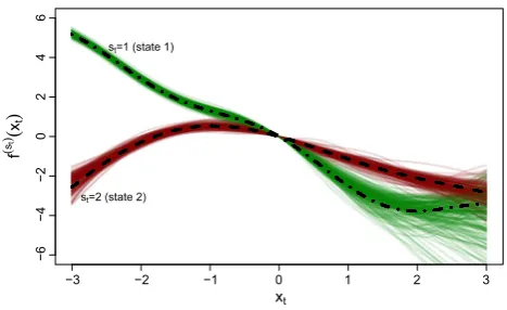
The functional forms of the predictors were chosen arbitrarily as

f(1)(xt)=0.3xt2+sin(−xt)

and

f(2)(xt)= −0.5−1.4xt+0.1xt2

+0.6 sin(−xt)+0.5 cos(2xt);

these functions are displayed by the dashed curves in Fig.1. Both functions go through the origin. We further setβ₀(1) = β(2)

0 =2 and

=

0.9 0.1 0.1 0.9

.

All covariate values were drawn independently from a uni-form distribution on [−3,3]. We ran 200 simulations, in each run generatingT =300 observations from the model

−3 −2 −1 0 1 2 3

−6

−4

−2

0

2

4

6

xt

f

(

st

) (x

t

)

(state 1) st=1

st=2 (state 2)

Fig. 1 Displayed are the true functionsf(1)_andf(2)_{used inScenario I} (dashed lines) and their estimates obtained in 200 simulation runs (green andred linesfor states 1 and 2, respectively). (Color figure online) described. An MS-GAM, with Poisson-distributed response and log-link, was then fitted via numerical maximum penal-ized likelihood estimation as described in Sect. 2.4above. We setK =15, hence using 15 B-spline basis densities in the representation of each functional estimate.

We implemented both generalized cross-validation and the AIC-based approach for choosing the smoothing para-meter vector from a grid=1×2, where1=2=

{0.125,1,8,64,512,4096}, consideringC = 25 folds in the cross-validation. For both approaches, we estimated the mean integrated squared error (MISE) for the two functional estimators, as follows:

MISE_f(j) = 1

200

200

z=1 3

−3

ˆ

fz(j)(x)− f(j)(x)

2

d x

,

for j = 1,2, where fˆz(j)(x)is the functional estimate of f(j)(x)obtained in simulation runz. Using cross-validation, we obtained MISE_f(1) = 1.808 and MISEf(2) = 0.243,

while using the AIC-type criterion we obtained the slightly better valuesMISEf(1) =1.408 andMISE_f(2) =0.239. In

the following, we report the results obtained using the AIC-based approach.

The sample mean estimates of the transition probabilities γ11andγ22 were obtained as 0.894 (Monte Carlo standard

deviation of estimates: 0.029) and 0.896 (0.032), respec-tively. The estimated functions fˆ(1) and fˆ(2) from all 200 simulation runs are visualized in Fig.1. The functions have been shifted so that they go through the origin. All fits are fairly reasonable. The sample mean estimates of the predictor value forxt =0 were obtained as 2.002 (0.094) and 1.966 (0.095) for states 1 and 2, respectively.

3.2 Scenario II

−3 −2 −1 0 1 2 3

−6

−4

−2

0

2

4

6

x1t

f1

(

st

) (x

1t

)

st=1 (state 1)

st=2 (state 2)

−3 −2 −1 0 1 2 3

−6

−4

−2

0

2

4

6

x2t

f2

(

st

) (x

2t

)

st=1 (state 1)

st=2 (state 2)

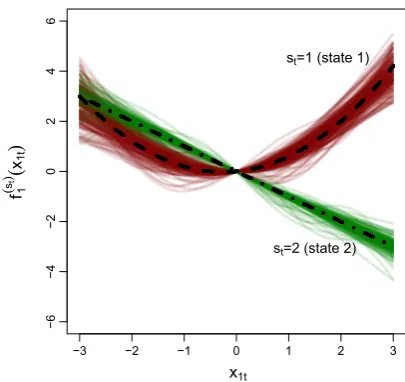
Fig. 2 Displayed are the true functionsf₁(1),f₁(2),f₂(1)and f₂(2)used in Scenario II(dashed lines) and their estimates obtained in 200 simulation runs (redandgreen linesfor states 1 and 2, respectively;f₁(1)and f₁(2), which describe the state-dependent effect of the covariatex1t on the

predictor, and corresponding estimates are displayed in theleft panel; f₂(1)and f₂(2), which describe the state-dependent effect of the covariate x2ton the predictor, and corresponding estimates are displayed in the

right panel). (Color figure online)

an underlying 2-state Markov chain and now two covariates:

Yt ∼N(μ(st)

t , σst),

where

μ(st) t =β(

st)

0 + f(

st)

1 (x1t)+ f(

st)

2 (x2t).

The functional forms were chosen as

f₁(1)(x1t)=0.2x1t +0.4x12t, f(

2)

1 (x1t)= −x1t,

f₂(1)(x2t)=x2t+1.2 sin(x2t) and

f₂(2)(x2t)= −0.2x2t−0.25x22t−sin(x2t);

see Fig.2. Again all functions go through the origin. We further setβ₀(1)=1,β₀(2)= −1,σ1=3,σ2=2 and

=

0.95 0.05 0.05 0.95

.

The covariate values were drawn independently from a uni-form distribution on[−3,3]. In each of 200 simulation runs,

T =1000 observations were generated.

For the choice of the smoothing parameter vector, we con-sidered the grid = 1×2×3×4, where1 =

2 = 3 = 4 = {0.25,4,64,1024,16384}. The

AIC-based smoothing parameter selection led to MISE estimates that overall were marginally lower than their counterparts obtained when using cross-validation (0.555 compared to 0.565, averaged over all four functions being estimated), so again in the following we report the results obtained based on the AIC-type criterion. The (true) function f(2)is in fact

a straight line, and, notably, the associated smoothing para-meter was chosen as 16384, hence as the maximum possible value from the grid considered, in 129 out of the 200 cases, whereas for example for the function f₂(2), which has a mod-erate curvature, the value 16384 was not chosen even once as the smoothing parameter.

In this experiment, the sample mean estimates of the transition probabilitiesγ11 andγ22 were obtained as 0.950

(Monte Carlo standard deviation of estimates: 0.011) and 0.948 (0.012), respectively. The estimated functions fˆ₁(1),

ˆ

f₁(2),fˆ₂(1)andfˆ₂(2)from all 200 simulation runs are displayed in Fig.2. Again all have been shifted so that they go through the origin. The sample mean estimates of the predictor value for x1t =x2t =0 were 0.989 (0.369) and−0.940 (0.261)

for states 1 and 2, respectively. The sample mean estimates of the state-dependent error variances,σ1andσ2, were obtained

as 2.961 (0.107) and 1.980 (0.078), respectively. Again the results are very encouraging, with not a single simulation run leading to a complete failure in terms of capturing the overall pattern.

3.3 Scenario III

−3 −2 −1 0 1 2 3

−6

−4

−2

0

246

xt

f

(

st

)(x

t

)

st=1 (state 1)

st=2 (state 2)

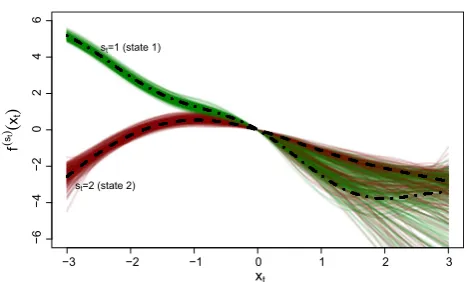
Fig. 3 Displayed are the true functions f(1)andf(2)used inScenario III(dashed lines) and their estimates obtained in 200 simulation runs (green andred linesfor states 1 and 2, respectively). (Color figure online)

=

0.6 0.4 0.4 0.6

.

In other words, compared toScenario I, there is substantially less autocorrelation in the series that are generated.

Figure3displays the estimated functions fˆ(1) and fˆ(2)

in this slightly modified scenario. Due to the fairly low level of autocorrelation, the estimator performance is substantially worse than inScenario I, and in several simulation runs the model failed to capture the overall pattern, by allocating pairs (yt,xt) with high values of the covariatext to the wrong state of the Markov chain. The deterioration in the estimator performance is also reflected by higher standard errors: The sample mean estimates of the transition probabilitiesγ11and

γ22were obtained as 0.590 (Monte Carlo standard deviation

of estimates: 0.082) and 0.593 (0.088), respectively, and the sample mean estimates of the predictor value forxt =0 were obtained as 1.960 (0.151) and 2.017 (0.145) for states 1 and 2, respectively.

4 Real data examples

4.1 Advertising data

We first consider a classic data set on Lydia Pinkham’s annual sales and advertising expenditures during the period 1907– 1960. The data set and its background are described in detail inPalda(1965). It comprises the sales in yeart,yt, and the annual advertising expenditures,xt, of the company. Both figures are given in millions of U.S. dollars. The time series of annual sales displays two distinct peaks, in 1925 and 1945, respectively (see Fig. 1 inPalda 1965). Statistical analyses of such data can aid managers in determining the effectiveness of advertising (Smith et al. 2006).

As a baseline parametric Markov-switching model, we consider the model formulation suggested bySmith et al.

(2006):

yt =β(st)

0 +β(

st)

1 xt+β(

st)

2 yt−1

+σstt, t =1908, . . . ,1960,

where t ii d

∼ N(0,1)and wherest is the state of a 2-state (stationary) Markov chain. This model, which involves 10 parameters, will be labeled MS-LIN in the following. Via numerical maximum likelihood, we obtained parameter esti-mates indicating that advertising was more effective in the model’s state 1 than in state 2 (β₁(1) = 0.746 > 0.397 = β(2)

1 ), with state 2 involving a stronger carryover effect

(β₂(2) =0.562 >0.434 =β₂(1)). For the given model, the Viterbi algorithm allocated the years 1917–1924 and 1939– 1944 to state 1, and all other years to state 2. The first switch to the state involving more effective advertising—i.e. the entry to state 1 in 1916/1917—followed the re-labeling of Lydia Pinkham’s Vegetable Compound, which had been advertised as an almost universal remedy prior to 1914, and was now being sold primarily as a relief of “female troubles” (Palda 1965). A possible reason for the first departure from the state with the more effective advertising—i.e. the departure from state 1 in 1924/1925—could be the fact that in 1925 Lydia Pinkham was ordered to stop advertising their Vegetable Compound as acting “directly upon female organs”, such that they labeled it as “vegetable tonic” instead, which led to a drop in sales (Palda 1965). Similarly, the re-entering of state 2 in 1938/1939 could be related to the Federal Trade Commission re-allowing Lydia Pinkham to use their ear-lier, more effective marketing strategy in 1940. From 1946 onwards, sales plummeted due to a changed general percep-tion of Lydia Pinkham as a “pseudoremedy from the previous century” (Applegate 2012), and this may explain the switch back to state 2. These findings are notably different to those given in Smith et al. (2006), who reported only one state switch, such that their model’s two regimes divided the data into a pre-war and a post-war period. We note that Smith et al.(2006) analyzed a slightly shorter data set, covering the period 1914–1960. However, we obtained different results— very similar to those reported here—also when fitting the model to that shorter series.

Next we fitted the following MS-GAM to the advertising data:

yt =β(st)

0 + f(

st)(_xt)+β(st)

1 yt−1

+σstt, t=1908, . . . ,1960,

again witht ii d

∼ N(0,1). This formulation is a semiparamet-ric version of the general MS-GAM formulation, where we nonparametrically model the effect of the advertising expen-diture xt but assume a simple linear effect of the previous year’s sales,yt₋1, on the current year’s sales,yt. This model

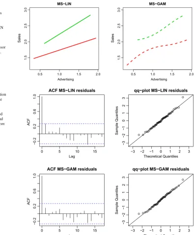
rel-Fig. 4 Lydia Pinkham data example: estimated

state-dependent mean sales as functions of advertising expenditure (state 1 ingreen, state 2 inred), for the MS-LIN model (left plot) and for the MS-GAM (right plot). Displayed are the predictor values when fixing the regressor yt−1at its overall mean, 1.84.

(Color figure online)

0.5 1.0 1.5 2.0

1.5 2 .0 2.5 3.0 MS−LIN Advertising Sales

0.5 1.0 1.5 2.0

1.5 2.0 2.5 3.0 MS−GAM Advertising Sales

Fig. 5 Lydia Pinkham data example: sample autocorrelation function and quantile-quantile plot (against the standard normal) of the forecast pseudo-residuals, for the fitted MS-LIN model (top plots) and for the fitted MS-GAM (bottom plots)

0 5 10 15

−0.2 0.2 0.6 1 .0 Lag AC F

ACF MS−LIN residuals

● ●● ● ● ● ● ● ● ● ● ● ● ● ● ● ● ● ● ● ● ● ● ● ● ● ● ● ● ●● ● ● ● ● ● ● ● ● ● ●● ● ● ● ● ● ●● ● ● ● ●

−3 −2 −1 0 1 2 3

−3

−2

−1

0123

qq−plot MS−LIN residuals

Theoretical Quantiles

Sample Quantiles

0 5 10 15

−0.2 0.2 0 .6 1.0 Lag AC F

ACF MS−GAM residuals

● ●● ● ● ● ●● ● ● ● ● ● ● ● ● ● ● ● ● ● ● ● ● ● ● ● ● ● ● ● ● ● ● ● ● ● ● ● ● ● ● ● ● ● ● ● ● ● ● ● ● ●

−3 −2 −1 0 1 2 3

−3

−2

−1

0

123

qq−plot MS−GAM residuals

Theoretical Quantiles

Sample Quantiles

atively parsimonious model formulation as the fairly short time series does not contain sufficient information to fit the fully nonparametric model (i.e. also allowing for nonpara-metric effects ofyt₋1).

Figure4 compares the estimated effect of the advertis-ing expenditure on the sales usadvertis-ing the MS-LIN model and the MS-GAM, respectively. Overall, the regression structure within the two states is very similar for the two differ-ent models. In particular, for the MS-GAM considered, the Viterbi-decoded state sequence is identical to that obtained using the LIN model. However, the more flexible MS-GAM does reveal some interesting nuances. In particular, for

state 2 there is a strong indication of a wearout effect in the benefits of advertising, suggesting that further increases of already high advertising expenditures do not increase sales as much as would be expected if a linear relation was assumed. This phenomenon is well-known in marketing (see, e.g.,

Corkindale and Newall 1978,Bass et al. 2007).

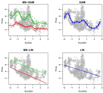
Fig. 6 Spanish energy prices example: observed energy price against Euro/Dollar exchange rate (gray points), with estimated state-dependent mean energy prices (solid lines) for one-state (blue) and two-state (greenandred) nonparametric and linear models;

nonparametric models are shown together with associated approximate 95 % pointwise confidence intervals obtained based on 999 parametric bootstrap samples (dotted lines). (Color figure online)

−2 −1 0 1 2 3

2468

MS−GAM

EurDol

Pr

ice

−2 −1 0 1 2 3

24

6

8

GAM

EuroDol

Pr

ice

−2 −1 0 1 2 3

2468

MS−LIN

EuroDol

Pr

ice

−2 −1 0 1 2 3

246

8

LIN

EuroDol

Pr

ice

the forward variables, are approximately standard normally distributed if the model is adequate (Zucchini and

Mac-Donald 2009). Overall, both models appear to fit the data

adequately. However, for the parametric MS-LIN model there is some residual autocorrelation, which is often an indication that more states are required to fully capture the correlation structure of the time series (under the given model formulation). No such lack of fit is observed for the MS-GAM.

4.2 Spanish energy prices

Next we analyze the data collected on the daily price of energy in Spain between 2002 and 2008. The data, 1784 observations in total, are available in the R packageMSwM

(Sanchez-Espigares et al. 2014). We consider the relation-ship over time between the price of energy, yt, and the Euro/Dollar exchange rate,xt. The commonly observed sto-chastic volatility of financial time series renders it unlikely that the relationship between these two variables is constant over time, and a possible, computationally efficient way to account for this is to consider a Markov-switching model. It is also probable that the two variables’ unknown relation-ship within a regime has a non-linear functional form. As in the previous example, in the following we illustrate potential advantages of considering Markov-switching models with

flexible nonparametric predictor functions, i.e. MS-GAMs, rather than GAMs or parametric Markov-switching models when analyzing time series regression data.

To this end, we consider four different models for the energy price data. As benchmark models, we considered two parametric models with state-dependent linear predic-torβ(st)

0 +β(

st)

1 xt, with one (LIN) and two states (MS-LIN),

respectively, assuming the response variable yt to be nor-mally distributed with state-dependent variance. Addition-ally, we considered two nonparametric models as introduced in Sect. 2.3, with one state (hence a basic GAM) and two states (MS-GAM), respectively. In these two models, we assumed yt to be gamma-distributed, applying the log link function to meet the range restriction for the (positive) mean. Figure6shows the fitted curves for each model. For each one-state model (GAM and LIN), the mean curve passes through a region with no data (for values ofxt around−1). This results in response residuals with clear systematic devi-ation. It is failings such as this which demonstrate the need for regime-switching models.

Models were also formally compared using an out-of-sample one-step-ahead forecast evaluation, by means of the sum of the log-likelihoods of observations yu under the models fitted to all preceding observations, y1, . . . ,yu₋1,

0 500 1000 1500

Time

258

Pr

ice (MS−GAM)

258 Pr

ice (MS−LIN)

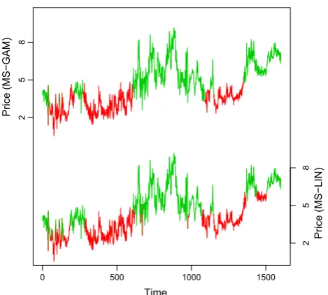
Fig. 7 Spanish energy prices example: globally decoded state sequence for the two-state (red and green) MS-LIN model and the two-state MS-GAM. (Color figure online)

the following log-likelihood scores for each model:−2314 for LIN,−2191 for GAM,−2069 for MS-LIN and−1703 for MS-GAM. Thus, in terms of out-of-sample forecasts, the MS-GAM performed much better than any other model con-sidered. Both two-state models performed much better than the single-state models, however the inflexibility of the MS-LIN model resulted in a poorer performance than that of its nonparametric counterpart, as clear non-linear features in the regression data are ignored.

For the MS-GAM, the transition probabilities were esti-mated to beγ11 =0.991 (standard error: 0.006) andγ22 =

0.993 (0.003). The estimated high persistence within states gives evidence that identifiability problems such as those encountered inScenario IIIin the simulation experiments did not occur here. Figure7gives the estimated regime sequence from the MS-GAM and the MS-LIN model obtained using the Viterbi algorithm. Both sequences are similar, with one state relating to occasions where price is more variable and generally higher. However, the MS-LIN model does tend to predict more changes of regime than the MS-GAM, which may be a result of its inflexibility.

While this second example is simplistic—for example, other explanatory covariates such as the oil price will also heavily affect the energy price—it nevertheless does illustrate the substantially increased flexibility, and hence increased potential to fit the data at hand, of MS-GAMs compared to their simpler parametric counterparts. At the very least, these models can prove useful as exploratory tools to identify key features in time series data with regime-switching patterns, without making any restrictive assumptions on the functional relationships a priori.

5 Concluding remarks

We have exploited the strengths of the HMM machinery and of penalized B-splines to develop a flexible new class of models, MS-GAMs, which show promise as a useful tool in time series regression analysis. A key strength of the inferential approach is ease of implementation, in par-ticular the ease with which the code, once written for any MS-GAM, can be modified to allow for various model for-mulations. This makes interactive searches for an optimal model among a suite of candidate formulations practically feasible. Model selection, although not explored in detail in the current work, can be performed along the lines ofCeleux and Durand(2008) using cross-validated likelihood, or can be based on AIC-type criteria such as the one we considered for smoothing parameter selection. For more complex model formulations, local maxima of the likelihood can become a challenging problem. In this regard, estimation via the EM algorithm, as suggested inSouza and Heckman(2014) for a smaller class of models, could potentially be more robust (cf. Bulla and Berzel 2008), but is technically more chal-lenging, not as straightforward to generalize and hence less user-friendly (MacDonald 2014).

There are various other ways to modify or extend the approach, in a relatively straightforward manner, in order to enlarge the class of models that can be considered. First, as already seen in the application to advertising data, it is of course straightforward to consider semiparametric ver-sions of the model, where some of the functional effects are modeled nonparametrically and others parametrically. Espe-cially for complex models, with high numbers of states and/or high numbers of covariates considered, this can improve numerical stability and decrease the computational burden associated with the smoothing parameter selection. Second, the consideration of interaction terms in the predictor is possi-ble via the use of tensor products of univariate basis functions. Third, the likelihood-based approach also allows for the consideration of more involved dependence structures (e.g. semi-Markov state processes;Langrock and Zucchini 2011). In particular, in the current model formulation we assume that a single univariate state process determines the GAM, such that changes in the state process affect all GAM parameters simultaneously. Conceptually there is no difficulty in devis-ing models where different parts of the GAM are driven by different Markov state processes. However, with such models the dimensionality of the state process and hence the com-putational burden will increase rapidly. Finally, in case of multiple time series, random effects can be incorporated into a joint MS-GAM formulation.

Open Access This article is distributed under the terms of the Creative Commons Attribution 4.0 International License (http://creativecomm ons.org/licenses/by/4.0/), which permits unrestricted use, distribution, and reproduction in any medium, provided you give appropriate credit to the original author(s) and the source, provide a link to the Creative Commons license, and indicate if changes were made.

References

Applegate, E.: The Rise of Advertising in the United States: A History of Innovation to 1960. Scarecrow Press, Lanham (2012) Bass, F.M., Bruce, N., Majumdar, S., Murthi, B.P.S.: Wearout effects

of different advertising themes: a dynamic Bayesian model of the advertising-sales relationship. Mark. Sci.26, 179–195 (2007) Bulla, J., Berzel, A.: Computational issues in parameter estimation for

stationary hidden Markov models. Comput. Stat.13, 1–18 (2008) Celeux, G., Durand, J.-P.: Selecting hidden Markov model state number with cross-validated likelihood. Comput. Stat.23, 541–564 (2008) Corkindale, D., Newall, J.: Advertising thresholds and wearout. Eur. J.

Mark.12, 329–378 (1978)

de Boor, C.: A Practical Guide to Splines. Springer, Berlin (1978) de Souza, C.P.E., Heckman, N.E.: Switching nonparametric regression

models. J. Nonparametric Stat.26, 617–637 (2014)

Efron, B., Tibshirani, R.J.: An Introduction to the Bootstrap. Chapman & Hall/CRC, New York (1993)

Eilers, P.H.C., Marx, B.D.: Flexible smoothing with B-splines and penalties. Stat. Sci.11, 89–121 (1996)

Fahrmeir, L., Kneib, T., Lang, S., Marx, B.: Regression: Models, Meth-ods and Applications. Springer, Berlin (2013)

Frühwirth-Schnatter, S.: Finite Mixture and Markov Switching Models. Springer, New York (2006)

Gassiat, E., Cleynen, A., Robin, S.: Inference in finite state space non parametric Hidden Markov models and applications. Stat. Comput. (2015). doi:10.1007/s11222-014-9523-8

Gneiting, T., Raftery, A.E.: Strictly proper scoring rules, prediction, and estimation. J. Am. Stat. Assoc.102, 359–378 (2007)

Goldfeld, S.M., Quandt, R.E.: A Markov model for switching regres-sions. J. Econom.1, 3–16 (1973)

Gray, R.J.: Flexible methods for analyzing survival data using splines, with application to breast cancer prognosis. J. Am. Stat. Assoc. 87, 942–951 (1992)

Hamilton, J.D.: A new approach to the economic analysis of nonstation-ary time series and the business cycle. Econometrica57, 357–384 (1989)

Hamilton, J.D.: Regime-switching models. In: Durlauf, S.N., Blume, L.E. (eds.) The New Palgrave Dictionary of Economics, 2nd edn. Palgrave Macmillan, New York (2008)

Kim, C.-J., Piger, J., Startz, R.: Estimation of Markov regime-switching regression models with endogenous switching. J. Econom.143, 263–273 (2008)

Krivobokova, T., Kneib, T., Claeskens, G.: Simultaneous confidence bands for penalized spline estimators. J. Am. Stat. Assoc.105, 852–863 (2010)

Langrock, R., Zucchini, W.: Hidden Markov models with arbitrary state dwell-time distributions. Comput. Stat. Data Anal.55, 715–724 (2011)

Langrock, R., Kneib, T., Sohn, A., DeRuiter, S.L.: Nonparametric infer-ence in hidden Markov models using P-splines. Biometrics71, 520–528 (2015)

MacDonald, I.L.: Numerical maximisation of likelihood: a neglected alternative to EM? Int. Stat. Rev.82, 296–308 (2014)

Palda, K.S.: The measurement of cumulative advertising effects. J. Bus. 38, 162–179 (1965)

Psaradakis, Z., Spagnolo, F.: On the determination of the number of regimes in Markov-switching autoregressive models. J. Time Ser. Anal.24, 237–252 (2003)

Rigby, R.A., Stasinopoulos, D.M.: Generalized additive models for location, scale and shape. J. R. Stat. Soc. Ser. C54, 507–554 (2005) Sanchez-Espigares, J.A., Lopez-Moreno, A.: MSwM: Fitting Markov-Switching Models. R package version 1.2.http://CRAN.R-project. org/package=MSwM(2014)

Schnabel, R.B., Koontz, J.E., Weiss, B.E.: A modular system of algo-rithms for unconstrained minimization. ACM Trans. Math. Softw. 11, 419–440 (1985)

Smith, A., Naik, P.A., Tsai, C.-H.: Markov-switching model selec-tion using Kullback–Leibler divergence. J. Econom.134, 553–577 (2006)

Wang, P., Puterman, M.L.: Markov Poisson regression models for dis-crete time series. Part 1: Methodology. J. Appl. Stat.26, 855–869 (2001)

Wood, S.: Generalized Additive Models: An Introduction with R. Chap-man & Hall/CRC, Boca Raton (2006)