University of Warwick institutional repository: http://go.warwick.ac.uk/wrap This paper is made available online in accordance with
publisher policies. Please scroll down to view the document itself. Please refer to the repository record for this item and our policy information available from the repository home page for further information.
To see the final version of this paper please visit the publisher’s website. Access to the published version may require a subscription.
Author(s) Stewart, Neil; Chater, Nick; Stott, Henry P.; Reimers, Stian Article Title: Prospect relativity: How choice options influence decision under risk.
Year of publication: 2003
Running Head: PROSPECT RELATIVITY
Prospect Relativity: How Choice Options Influence Decision Under Risk
Neil Stewart, Nick Chater, Henry P. Stott, and Stian Reimers
University of Warwick
Stewart, N., Chater, N., Stott, H. P., & Reimers, S. (2003). Prospect relativity: How choice
options influence decision under risk. Journal of Experimental Psychology: General,
Abstract
In many theories of decision under risk (e.g., expected utility theory, rank-dependent utility
theory, and prospect theory), the utility of a prospect is independent of other options in the
choice set. The experiments presented here show a large effect of the available options,
suggesting instead that prospects are valued relative to one another. The judged certainty
equivalent for a prospect is strongly influenced by the options available. Similarly, the
selection of a preferred prospect is strongly influenced by the prospects available. Alternative
theories of decision under risk (e.g., the stochastic difference model, multialternative decision
field theory, and range frequency theory), where prospects are valued relative to one another,
Prospect Relativity: How Choice Options Influence Decision Under Risk
Decisions almost always involve trading off risk and reward. In crossing the road, one
balances the risk of accident against the reward of saving time; in choosing a shot in tennis,
one balances the risk of an unforced error against the reward of winning. Choosing a career, a
life partner, or whether to have children involves trading off different balances between the
risks and returns of the prospects available. Understanding how people decide between
different levels of risk and return is, therefore, a central question for psychology.
Understanding how people trade off risk and return is also a central issue for
economics. The foundations of economic theory are rooted in models of individual decision
making. For example, to explain the behavior of markets one needs a model of the
decision-making behavior of buyers and sellers in those markets. Most interesting economic decisions
involve risk. Thus, an economic understanding of markets for insurance, of risky assets such as
stocks and shares, of the lending and borrowing of money itself, and indeed of the economy at
large requires understanding how people trade risk and reward.
In both psychology and economics, the starting point for investigating how people
make decisions involving risk has not been empirical data on human behavior. Instead, the
starting point has been a normative theory of decision making, expected utility (hereafter, EU)
theory (axiomatized by von Neumann & Morgenstern, 1947), which specifies how people
ought to make decisions and plays a key role in theories of rational choice (for a review, see
Shafir & LeBoeuf, 2002). The assumption has then been that, to an approximation, people do
make decisions as they ought to, that is, that EU theory can be viewed as a descriptive, as well
as a normative, theory of human behavior (Arrow, 1971; Friedman & Savage, 1948). At the
core of EU theory are the assumptions that people make choices that maximize their utility
and that they value a risky option by the EU (in a probabilistic sense of expectation) that it will
provide. In general, the prospect (x1, p1; x2, p2; ... ; xn, pn), where outcome xi occurs with
U x1, p1; x2, p2;...; xn, pn= p1u x1 p2u x2... pnu xn (1)
(The function U gives the utility of a risky prospect. The function u is reserved for the utility
of certain outcomes only.)
In psychology and experimental economics, there has been considerable interest in
probing the limits of this approximation, that is, in finding divergence or agreement between
EU theory and actual behavior (see, e.g., Kagel & Roth, 1995; Kahneman, Slovic, & Tversky,
1982; Kahneman & Tversky, 2000). It is now well established that people systematically
violate the axioms of EU theory (see Camerer, 1995; Luce, 2000; Schoemaker, 1982, for
reviews). In economics more broadly, there has been interest in how robustly economic theory
copes with anomalies between EU theory and observed behavior (for a range of views, see,
e.g., Akerlof & Yellen, 1985; Cyert & de Groot, 1974; de Canio, 1979; Friedman, 1953;
Nelson & Winter, 1982; Simon, 1959, 1992).
The present article demonstrates a new and large anomaly for EU theory in decision
making under risk. Specifically, we report results that seem to indicate that people do not
possess a well-defined notion of the utility of a risky prospect and hence, a fortiori, do not
view such utilities in terms of EU. Instead, people's perceived utility for a risky prospect
appears highly context sensitive. We call this phenomenon prospect relativity.
Motivation From Psychophysics
In judging risky prospects, people must assess the magnitudes of risk and return that
the prospects comprise. The motivation for the experiments presented here was the idea that
some of the factors that determine how people assess these magnitudes might be analogous to
factors underlying assessment of psychophysical magnitudes, such as loudness or weight.
Specifically, people appear poor at providing stable absolute judgments of such magnitudes
and are heavily influenced by the options available to them. For example, Garner (1954) asked
participants to judge whether tones were more or less than half as loud as a 90-dB reference
them. Participants played tones in the range 55-65 dB had a half-loudness point, where their
judgments were more than half as loud 50% of the time and less than half as loud 50% of the
time, of about 60 dB. Another group, which received tones in the range 65-75 dB, had a
half-loudness point of about 70 dB. A final group, who heard tones in the range 75-85 dB, had a
half-loudness point of about 80 dB. Laming (1997) provided an extensive discussion of other
similar findings. Context effects, like those found by Garner, are consistent with participants
making perceptual judgments on the basis of relative magnitude information, rather than
absolute magnitude information (Laming, 1984, 1997; Stewart, Brown, & Chater, 2002a,
2002b). If the attributes of risky prospects behave like those of perceptual stimuli, then similar
context effects should be expected in risky decision making. This hypothesis motivated the
experiments in this article, experiments that were loosely based on Garner's procedure.
Existing Experimental Investigations
A few experiments have already investigated the effect of the set of available options in
decision under risk. Mellers, Ordóñez, and Birnbaum (1992) measured participants'
attractiveness ratings and buying prices (i.e., the price that a participant would pay to obtain a
single chance to play the prospect and have a chance of receiving the outcome) for a set of
simple binary prospects of the form "p chance of x." These experimental prospects were
presented with one of two sets of filler prospects. For one set of filler prospects, the
distribution of expected values was positively skewed, and for the other set, the distribution of
expected values was negatively skewed. Attractiveness ratings of the experimental prospects
were significantly influenced by the filler prospects, with higher ratings for prospects in the
positive skew condition than for the same prospects in the negative skew condition. However,
context had only a very small effect on buying price. With more complicated prospects of the
form "p chance of x otherwise y," the effect of skew on buying price was slightly larger. The
large effect that the set of options available had on attractiveness ratings and the much smaller
Lichtenstein (1999). They gave participants a set of prices for different brands of the same
product to study. The prices varied in range. The range had an effect on judgments of the
attractiveness of a new price but not on the amount participants reported that they would
expect to pay for a new product.
The set of options available as potential certainty equivalents (hereafter, CEs) has been
shown to affect the choice of CE for risky prospects. In making a CE judgment, participants
suggest or select from a set of options the amount of money for certain that is worth the same
to them as a single chance to play the prospect. We considered CE judgments extensively in
our experiments. Birnbaum (1992) demonstrated that skewing the distribution of options
offered as CEs for simple prospects, while holding the maximum and minimum constant,
influenced the selection of a CE. When the options were positively skewed (i.e., when most
values were small) prospects were undervalued compared to when the options were negatively
skewed (i.e., when most values were large).
MacCrimmon, Stanbury, and Wehrung (1980) presented some evidence that the set in
which a prospect is embedded can affect judgments about the prospect. They presented
participants with two sets of five prospects to be ranked in order of attractiveness. The
expected value of each prospect was constant across all prospects and both sets. There were
two prospects in common between the two sets. If context provided by the other prospects in
a set did not affect the attractiveness of a prospect, each participant should have consistently
ranked one prospect as more attractive than the other in both sets. MacCrimmon et al. found
that 9 of a total of 40 participants had a different ordering of the two prospects in the two
sets. They argued that this was not merely inconsistency, because these participants made
consistent rankings within a set, but instead reflected the influence of the other prospects in
the choice set. Following this logic, however, it would take only one participant who had a
different ordering of the two prospects but who otherwise behaved consistently to conclude
might produce this result. With such a small number of data points and no concrete null
hypothesis allowing a significance test to be made any conclusion based on this results must be
very tentative.
In summary, there is an effect of previously considered prospects on the attractiveness
rating assigned to a current prospect and also a small effect on buying price. Moreover, the
context provided by a set of values from which a CE is to be chosen affects CE judgments.
Finally, in choosing between prospects, there is a suggestion that other prospects in the choice
set may reverse preferences between identical pairs of prospects. In the experiments reported
below we found large and systematic effects of choice set (both potential CEs and
accompanying prospects) on the valuation of individual prospects. These effects are not
compatible with EU theory or some of its most influential variants, according to which the
value of a prospect is independent of other available options. These results are, though,
compatible with a variety of models that discard this independence assumption. We consider
such models in the General Discussion.
Summary of Experiments
As indicated above, in this study we adapt methodologies from psychophysics to
investigate the possibility that context effects influence decision under risk. The aim of
Experiments 1A-1D was to determine whether options offered as potential CEs influenced
estimates of a prospect's CE. We consistently found substantial effects. In Experiment 2, to
investigate these effects, we introduce a new procedure in which, under certain assumptions, it
was optimal for participants to provide truthful CEs. In Experiment 3, we examined whether
these effects were similar to those observed in magnitude estimation tasks. In the remaining
two experiments, Experiments 4 and 5, we investigated whether the effect of available options
arose in choices between prospects as well as in CE judgments about prospects.
Experiment 1A
above, we gave participants a set of four options as possible CEs for a series of prospects.
Participants were asked to decide on a CE for the prospect and then select the option closest
to their estimate. For each prospect, options were either all lower in value than the mean free
choice CE (given by another group of participants) or all higher.1 If participants were not
influenced by the set of options, then their choice of option should have been that nearest to
their free-choice CE. A key prediction of this hypothesis is that either the highest option of the
low options (L4), the lowest option of the high options (H1), or both should be chosen more
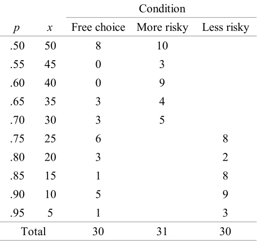
than half of the time. Consider the distribution of free-choice CEs illustrated in Figure 1A. If
H1 is to be selected less than half of the time, then the area to the left of the H1-H2 bound must
be less than one half. This area corresponds to the proportion of times that the free choice CE
is nearest to H1. Thus, the area to the right (labeled Area A) must be greater than one half.
This means that the proportion of times that L4 will be selected from the low options must be
greater than one half, as this proportion corresponds to the sum of area to the right of the H1
-H2 bound (Area A - which was greater that half) and the area between the L3-L4 and H1-H2
bounds (Area B - which depends on the exact probability density function, but must be greater
than or equal to zero). This argument is true for any probability density function. Similarly, if
L4 is selected less than half of the time, H1 must be selected more than half of the time (Figure
1B). The selection of L4 less than half of the time and H1 less than half of the time is not
consistent with any distribution of free-choice CEs that is not affected by context. If
participants' responses were solely determined by the set of options presented to them,
however, then the distribution of responses across options should have been the same for both
the low- and the high-value options.
Method
Participants. Free-choice CEs were given by 14 psychology undergraduates from the
University of Warwick. Another 16 psychology undergraduates chose CEs from sets of
participants were female.
Design. A set of 20 prospects, each of the form "p chance of x," was created by
crossing the amounts £200, £400, £600, £800, and £1000 with the probabilities .2, .4, .6,
and .8. In a pretest, 14 participants were asked to provide a CE for each prospect. The means
and standard deviations of the free choice CEs were calculated for each prospect (see
Appendix A).
For each prospect, two sets of options were created as follows. In the low-options
condition, the options were 1/6, 2/6, 3/6, and 4/6 of a standard deviation below the mean. In
the high options condition, options were 1/6, 2/6, 3/6, and 4/6 of a standard deviation above
the mean. Thus, the range of each set was half a standard deviation. Options were rounded to
have familiar, easy-to-deal-with values.
Sixteen new participants were presented with the prospects and options and asked to
select the option closest to their CE from a set of four. Eight participants received the low
options for every prospect. The other eight received the high options for every prospect. Note
that this method, in which a range of potential CEs is presented, is not uncommon in other
experimental work in this area (see, e.g., Tversky & Kahneman, 1992).
Procedure. Participants were asked to imagine choosing between "£30 for certain" or
a "50% chance of £100" to illustrate that prospects could have a value. They were told they
would be asked to value a series of prospects. It was explained that the purpose of the
experiment was to investigate how much they thought the prospects were worth and that there
were no correct answers. Participants were asked to choose the option nearest the value they
thought the prospect was worth to them.
Each prospect was presented on a separate page of a 20-page booklet. The ordering of
the prospects was random and different for each participant. Probabilities were always
presented as percentages. Options were always presented in numerical order, as in the
How much is the gamble
"60% chance of £400"
worth?
Is it: £60 £80 £100 £120
When collecting pretest free-choice CEs, the options were omitted, and a blank line on
which participants could write their CE was added.
Results
Participants took approximately 5 minutes to complete the task. Under free-choice
conditions, the average CE (see Appendix A) increased with both probability of winning and
the amount that could be won, demonstrating that participants were sensitive to manipulations
of both. The chosen CE was an approximately linear function of the independent effects of
prospect amount and prospect probability.
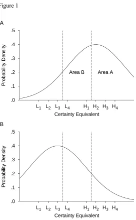
The proportion of times each option was chosen is plotted in Figure 2. The distribution
of options is approximately the same for the two conditions. L4 was chosen significantly less
than half the time, t(7) = 4.21, p = .0040 (2 = .72). The same was true of H
1, t(7) = 5.26, p =
.0012 (2 = .80). Thus the hypothesis that participants' CEs would be unaffected by context
can be rejected. (An alpha level of .05 was used for all statistical tests in this article, but for
informational value, we also report the exact p value of each test.2)
Discussion
CE judgments were strongly influenced by the CE options offered. These data
therefore appear to illustrate prospect relativity: People do not seem to form a stable absolute
judgment of the value of a prospect but instead choose an option relative to the options
available. The preference for central options in each set may be an example of extremeness
aversion (also called the compromise effect; see Simonson & Tversky, 1992). Indeed, these
data may reflect a more general tendency to prefer central options that is seen when choosing
Experiment 1B
A natural explanation of the effect of the set of options available in Experiment 1A is
that, on a given trial, the options available affected a participant's judgment. However, an
alternative and, for our purposes, less interesting explanation is that when participants were
repeatedly presented with trials containing too-high or too-low options, they learned to
readjust their judgments to fit their responses within the alternatives given. One way of ruling
out this alternative explanation was to use a within-participants design. In this design each
participant was presented with some trials on which all the options were lower than the
free-choice CE and others on which all the options were higher. If the effect seen previously had
been caused by participants learning to adjust their judgments up or down to fit into the
response scale, the effect should now have disappeared. However, if the effect was caused by
the options available on that trial only, then the pattern of results demonstrated in Experiment
1A should have been be replicated.
Method
Participants. Free-choice CEs were given by 35 volunteers. Twenty-eight different
volunteers chose CEs from sets of options. All participants were undergraduates or
postgraduates from the University of Warwick, and none had participated in Experiment 1A.
Ages ranged from 18 to 30 years, with a mean of 22 years. Two thirds of participants were
female. Participants were paid £5 for taking part in this and other related experiments.
Design and procedure. The design was the same as in Experiment 1 except that for
each participant, 10 trials were randomly selected to have options all higher than the pretest
mean for that prospect, the other 10 having options all below the mean. Trials were randomly
intermixed. Free-choice CEs and corresponding options are given in Appendix B. The
procedure was the same as in Experiment 1A.
Results
were excluded from the analysis because he had been given a misleading answer to a query
about the task that would have led to an inappropriate response strategy. As before, under free
choice, the CE increased approximately linearly with both the amount that could be won and
the probability of winning.
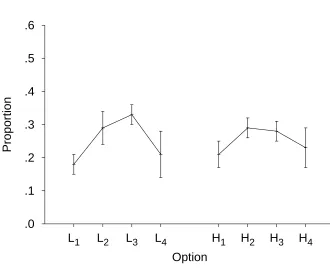
Figure 3 shows the proportion of choices of each option. In both conditions, the
proportion of responses increases with proximity to the mean free-choice CE. Planned t tests
showed that the proportions of L4 and H1 responses were significantly below .5, t(26) = 2.65,
p = .0135 (2 = .21), and t(26) = 3.81, p = .0008 (2 = .36), respectively.
A further issue is whether the context effects found in the main analysis applied to all
participants or whether some people showed a larger context effect than others. For each
participant, two scores were constructed, one for each condition. Participants were awarded
one point for each time they chose the lowest option, two for the next lowest, three for the
second highest, and four for the highest (i.e., scores were the rank of the options selected in
each condition). Those showing no effect of the option set should have chosen the L4 and H1.
However, those who based their judgment entirely on the option set would choose midrange
options. Thus, a negative correlation between low-choice CEs and high-choice CEs would be
evidence that people varied in the extent to which context influenced their CE decisions. Far
from being negatively correlated, there was a significant positive correlation (r2 = .45, p = .
0001). One interpretation of this positive correlation is that participants had a tendency to
choose an option with the same rank across the low- and high-choice CE conditions. (Note
that this analysis could not be run for Experiment 1A because the set of options was
manipulated between participants.)
Perhaps surprisingly, we found no evidence that the options offered on the previous
trial influenced the option selected on the current trial. One might imagine that, say, offering
low options on the previous trial might cause participants who were trying to be consistent to
rank (as described above) of the option selected within the set did not depend on the previous
option set offered (mean rank = 2.63, SE = 0.11, for prior low options vs. mean rank = 2.62,
SE = 0.13, for prior high options), t(26) = 0.23, p = .8407.This test is sufficiently sensitive to
be able to detect a difference of 0.21 between the mean ranks with a power of 80%.3
Discussion
As in Experiment 1A, participants' CE judgments in Experiment 1B were influenced, at
least in part, by the options from which the CE had to be chosen. In Experiment 1B, there was
a tendency to prefer higher options from the low CEs set and lower options from the high CEs
set. (This contrasts with Experiment 1A, where there was no such tendency.) Overall, the
pattern of results shown in Experiment 1B is intermediate between that expected under the
hypothesis that the available options are irrelevant and that expected if the available options
are the only determinant of responses. The tendency in Experiment 1B can be accounted for in
three ways. First, the effect in Experiment 1A may have been partly caused by participants
readjusting their responses to fit in with the options available. In Experiment 1B, such an
adjustment need not have been made as the option set was manipulated within participants,
and thus a smaller context effect was observed. However, this explanation still requires an
additional factor, such as prospect relativity, to contribute to the effects seen in Experiments
1A and 1B.
A second explanation of the tendency is that the absolute spacing of the options
differed between Experiments 1A and 1B. In both experiments, the spacing of CE options was
set at 1/6 of a free-choice SD. However, the free-choice SDs were smaller in Experiment 1B,
and thus, the absolute values of the options were actually more closely spaced in Experiment
1B.4 For this reason, we replicated Experiments 1A and 1B as conditions of a single
experiment, using the spacings from Experiment 1B throughout. The between-participants
result was similar to those of Experiment 1A and the within-participants result similar to those
of preferences in Experiments 1A and 1B in terms of using different options can thus be ruled
out.
A third explanation of the difference between Experiments 1A and 1B, and one that we
favor, is that participants may have been trying to be consistent with their responses to
previously completed questions. Thus, encountering both low and high CE options caused
participants to seem less affected by context. Such a consistency effect cannot be due to the
immediately preceding trial alone as there was no effect of the immediately preceding trial.
Instead, if this kind of explanation is correct, the tendency must be due to some larger window
of previous trials.
Experiment 1C
The effect of available options in Experiments 1A and 1B appears to create difficulties
for EU and related theories as descriptive accounts of decision under risk. Yet these
difficulties may be less pressing if the effects demonstrated thus far arose only because the
options presented as CEs were simply too close together, and that participants were roughly
indifferent between them. (Although note that this ought to lead to a u-shaped preference
across the options, rather than an n-shape.5) If this were the case then these effects should
disappear when the options are more widely spaced and hence are no longer indifferent
between them. In Experiment 1C, we investigated the effect of increasing the spacing of the
options.
Method
The method was the same as in Experiment 1B (i.e., low and high options were
presented within participants) except that there were three between-participants spacing
conditions. In the narrow condition, options were spaced at 1/6 of a free-choice standard
deviation as in Experiments 1A and B. In the wide condition, the spacing between adjacent
options was doubled to one third of a free-choice standard deviation, and thus the wide
means of the option sets. A gap condition was introduced, with the option spacing of the
narrow condition and the option group means of the wide condition. Thus, the gap condition
differed from the narrow condition only on the mean of the sets and from the wide condition
only on the spacing of the options. Eighteen undergraduate and postgraduate students from
the University of Warwick took part in the gap condition, and 19 in each of the narrow and
wide conditions. Ages ranged from 18 to 30 years, with a mean of 22 years. Two thirds of
participants were female.
Results
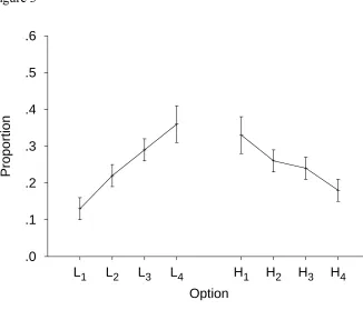
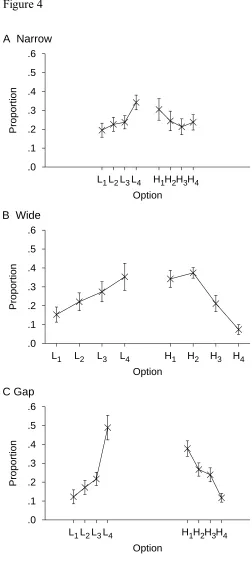
The proportion of times each option was selected is shown in Figure 4. In the narrow
condition, option L4 was selected significantly less than half the time, t(18) = 4.02, p = .0008
(2 = .47), as was the H
1 option, t(18) = 3.42, p = .0031 (2 = .39), replicating the results of
Experiment 1B. In the wide condition, option L4 was selected less than half the time, t(18) =
2.04, p = .0565 (2 = .19), although this difference is only marginally significant. The H 1
option was selected significantly less than half of the time, t(18) = 3.52, p = .0024 (2 = .41).
The key result is that doubling the spacing of the options did not eliminate the context effect.
In the gap condition, L4 was not chosen significantly less than half of the time, t(17) = 0.17, p
= .8665, but H1 was, t(17) = 2.99, p = .0082 (2 = .34).
The differences between the conditions were examined with a two-way (Condition x
Option Set) univariate analysis of variance (ANOVA), with the mean rank of the option
selected as the dependent measure. (It was not possible to run a Condition x Option Set x
Option ANOVA, as the selection of options was not independent: The proportion of times
each option was selected must sum to 1.) There was no significant main effect of condition,
F(2, 53) < 1.00. There was a significant main effect of set, F(1, 53) = 56.16, p < .0001 (2
= .51). Participants chose options with higher ranks in the low-options condition compared
with the high-options condition. The interaction was also significant, F(2, 53) = 4.00, p = .
0241 (2 = .13). The tendency to prefer L
than the other conditions. To examine the interaction further, we ran a one-way univariate
ANOVA with condition as a factor and the difference in ranks between the low and high
options as the dependent measure. Ryan REGWQ post hoc tests revealed that the tendency to
respond with high-ranking low options and low-ranking high options (i.e., the central
tendency) was significantly smaller for the narrow condition, with no difference between the
wide and gap conditions.
There was a marginally significant positive correlation between the mean rank of the
options selected in the low- and high-options trials in the narrow-option spacing condition, r2
= .20, t(17) = 2.07, p = .0543. This replicates the correlation seen in Experiment 1B. This
correlation was not seen in the wide, r2 = .01, t(17) = 0.45, p = .6574, and gap conditions, r2 =
.05, t(16) = 0.95, p = .3570. A correlation of r2 .35 can be detected with 80% power in this
design. Despite the failure to find positive correlations in the wide and gap conditions, there is
reason to think the positive correlations seen in the narrow condition of this experiment and in
Experiment 1B are reliable: We have replicated the correlation in the replication of
Experiments 1A and 1B reported in the discussion of Experiment 1B and also in a further,
unpublished study.
As in Experiment 1B, we investigated whether there was an effect of the option set
offered on the previous trial on the option selected on the current trial. A two-way (Condition
x Previous Option Set) ANOVA was run, with the rank of the option selected on the current
trial as the dependent measure. There was no significant main effect of condition, F(2, 53) =
1.38, p = .2601. As in Experiment 1B, there was no significant main effect of the previous
option set, F(1, 53) < 1.00 (mean rank of option selected on current trial with low options on
the previous trial = 2.51, SE = 0.05, vs. a mean rank = 2.50, SE = 0.07, with high options of
the previous trial). (A single t test for the difference in mean ranks between the low- and
high-option sets can detect a difference of .17 with a power of 80%.) There was no significant
Discussion
The effect of the options offered as CEs seen in Experiment 1B was replicated in the
narrow condition of Experiment 1C. Doubling the spacing of the options in the wide condition
did not eliminate the effect. However, there was a greater tendency to select lower options
from the high set and higher options from the low set in the wide and gap conditions when the
difference between the means of the option sets was larger. We consider two possible
accounts of this result. First, increasing the set mean spacing may have caused participants to
rely more on some representation of the absolute utility of each prospect. Perhaps this might
be because they realized that the options were quite different from some approximate
representation of the utilities of the prospects. However, in this case one might have expected
the effect to be larger in the wide rather than the gap condition as the wide condition
contained the more disparate options. In fact, the difference, although nonsignificant, was in
the opposite direction. A second explanation is that increasing the spacing of the set means
should have increased a consistency effect where participants tried to give consistent answers
across the low- and high-option sets. Both explanations offer an account of the lack of a
correlation between the rank of the options selected across the low- and high-option sets for
the wide and gap conditions. Consistency between the low- and high-option sets should have
caused participants to select low options from the high set and high options from the low set,
as should an increased reliance upon the prospects' absolute utilities. Thus, consistency should
have caused a negative correlation that would have acted in opposition to the positive
correlation observed in Experiment 1B and the narrow condition here, leaving a net zero
correlation.
Experiment 1D
Experiment 1D aimed to discriminate between the two explanations of the tendency to
select L4 options from the low set and H1 options from the high set seen in the wide and gap
and high sets, then repeating the experiment with option set as a between-participants variable
should have eliminated the effect. Alternatively, if the wider spacing somehow caused
participants to rely more on some representation of absolute utilities, then the greater central
tendency should also have been seen in the wide spacing condition even if a given participant
saw only low options or only high options. For this reason, in Experiment 1D, option set
manipulated between participants.
Method
Participants. Sixty professionals attending a conference at the University of Warwick
were approached on the campus and asked to participate. Participants' ages ranged between
20 and 40 years, with a mean of 27 years. An approximately equal number of male and female
participants took part.
Design and procedure. Spacing (narrow or wide) and option set (low or high) were
manipulated between participants: Fifteen participants took part in each condition. In the wide
condition, the low options were set at .10, .20, .30, and .40 of the expected value of each
gamble. The high options were set at .60, .70, .80, and .90 of the expected value. In the
narrow condition, the interval between options was halved. The low options were set at .30, .
35, .40, and .45 of the expected value. The high options were set at .55, .60, .65, and .70 of
the expected value. In other respects, the procedure was the same as in previous experiments.6
Results
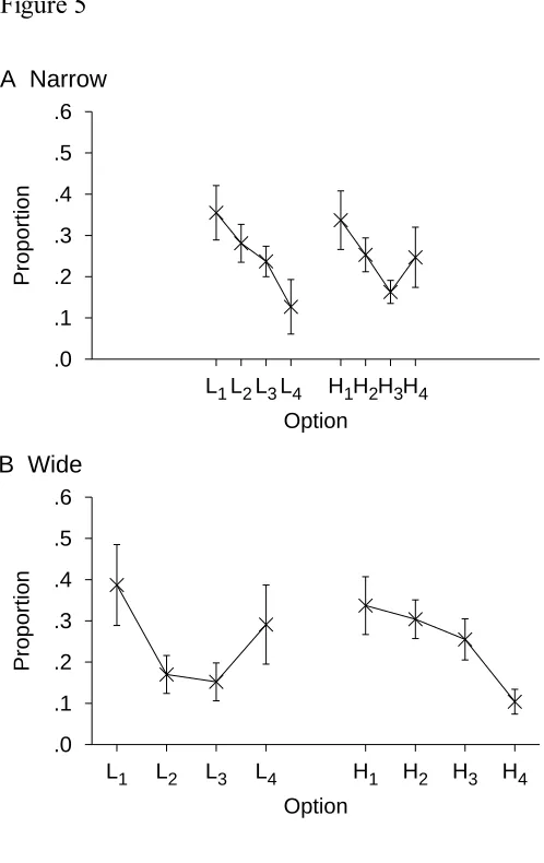
The proportion of times each option was selected is shown in Figure 5. Overall, there
was a preference for the lowest options. This was caused by some participants stating that
they did not gamble and then selecting the lowest option on every trial. In the narrow
condition, option L4 was selected significantly less than half the time, t(14) = 5.69, p = .0001
(2 = .70), as was the H
1 option, t(14) = 2.31, p = .0368 (2 = .28), replicating the results of
Experiment 1A. In the wide condition, option L4 was selected less than half the time, t(14) =
2.17, p = .0477 (2 = .25), as was the H
the spacing of the options did not eliminate the context effect. As in Experiment 1C, a
two-way (Spacing x Option Set) ANOVA was run, with the mean rank of the option selected as
the dependent measure. There was no main effect of spacing, F(1, 56) < 1. In contrast with
Experiment 1C, there was no main effect of option set, F(1, 56) < 1, and no interaction, F(1,
56) < 1. As option set was manipulated between participants the correlation across option sets
and the effect of the option set on the previous trial could not be examined.
Discussion
In Experiment 1C, where option set was manipulated within participants, there was a
greater tendency to prefer L4 and H1 when the options were widely spaced. However, such a
tendency was not evident here, when option set was manipulated across participants. Thus,
not all of the central tendency evident in Experiment 1C can be attributed to participants
relying more on some representation of absolute utilities: Instead, at least some of this effect
must be due to consistency across option sets.
Summary of Experiments 1A-1D
To sum up thus far, Experiment 1A demonstrated that the options presented as CEs
had a large effect on CE judgments for simple prospects. In Experiment 1B, the set of options
was manipulated within participants to investigate whether the results of Experiment 1A might
be due to participants adjusting their CE estimates over the course of the experiment to fit in
with the options offered. However, the context effect remained. In Experiment 1C, the spacing
of the options was increased to investigate the limits of this prospect relativity. However, even
when the options were widely spaced, there was an effect of option set. A greater tendency to
prefer high options from the set of low options and low options from the set of high options
was seen when options were more widely spaced. In Experiment 1D, the greater tendency was
not observed when the different option sets were presented across participants. This suggests
that the tendency was due, at least in part, to participants attempting to be consistent across
representation of absolute utilities.
Experiment 2
In Experiments 1A-1D, the set of options offered as CEs affected the CE selected.
Experiment 2 was designed to demonstrate the same effect of restricting the range of CE
options in a task where it was optimal for participants to report CEs truthfully. Although
psychologists typically assume that participants are honest when providing hypothetical CEs,
economists are typically concerned with providing a system of incentives that ensures it is
optimal for participants to provide truthful CEs. Hence, the results above may be criticized
from an economic perspective.
There is evidence that psychologists are correct in their assumption that participants
are typically honest in their judgments. For example, Lichtenstein and Slovic (1971)
demonstrated preference reversals in choices between two prospects and in CE estimates for
those prospects in situations where decisions were hypothetical and in situations where there
was an incentive system (see also Tversky, Slovic, & Kahneman, 1990). Preference reversals
have also been demonstrated with ordinary gamblers playing for high stakes in Las Vegas
(Lichtenstein & Slovic, 1973; see also Grether & Plott, 1979). For further discussion of these
and other similar findings, see Hertwig and Ortmann (2001) and Luce (2000, pp. 15-16).
However, because of the potential importance of the findings from Experiments 1A-1D for
models of economics, we include this experiment where the incentive system had been
designed to motivate participants to provide truthful CEs.
The design follows a solution to the cake-cutting problem, where a cake must be
divided fairly between two children. One solution is to allow one child to cut the cake into two
pieces and the other child to select the piece. The first child should cut the cake exactly in half,
otherwise the other child will take the larger piece of cake, leaving the first child with the
smaller piece.
an amount that could be be won with a known, fixed probability. For example, they might split
£1,000 into a sure amount of £300 and the prospect "60% chance of £700." Participants knew
that the other person (who was not the experimenter) would select either the prospect or the
sure amount, taking the better of the two, leaving the participant with the other. Thus, it was
optimal for participants to split the given amount so that they had no preference between the
resulting fixed amount and the resulting prospect. Note that this procedure works only if each
participant assumes that the chooser has the same level of risk preference as himself or herself.
To this end, participants were told to assume that the chooser did have the same risk
preference as they did.
This procedure is more simple than other methods used to elicit truthful CEs, for
example, the first price auction, or the Becker, DeGroot, and Marschak (BDM; 1964)
procedure. In the BDM procedure, participants are given the chance to play a prospect and
are asked to state the minimum price at which they would sell the prospect. A buying price is
then randomly generated by the experimenter, and if it exceeds the selling price, then the
prospect is bought from the participant. If not, then the participant plays the prospect. It is the
case that it is optimal for participants to state a selling price that is the CE of the prospect,
though it is unlikely that many participants realize this.
Method
Participants. Participants were psychology undergraduates from the University of
Warwick who had not participated in Experiments 1A-1D. Ages ranged from 18 to 25 years,
with a mean age of 20 years. The majority of participants were female. Seventeen participants
took part in the free-choice condition of the experiment. Nineteen further participants took
part in the restricted-choice conditions. Participants were paid £5, plus performance-related
winnings of up to £4.
Design. In each trial of the free-choice condition, participants divided a given amount
"p chance of z." Probability p was known to participants before splitting amount x.
Participants were told that one trial in the experiment would be selected at random at the end
of the experiment and that a second person would take either the fixed amount or the prospect
for himself, leaving the participant with the other option. Under the assumption that the
chooser had the same risk preference as they did, it was explained to participants that the
chooser would choose the option with greater utility, leaving the participants with their less
preferred option, if they did not split the amount to make options of equal utility. It was
therefore optimal for participants to split the amount x into amounts y and z such that y and a
"p chance of z" were equivalent for them, that is, that y was the CE for the prospect "p chance
of z."
The restricted-choice conditions differed by offering participants a choice from a set of
four pre-split options rather than giving them a completely free choice. That is, values for y
and z were presented, and participants selected one pair that could be played at the end of the
experiment. It could be argued that participants might reasonably think that the pairs of y and
z values presented might provide them with information about the chooser's risk preferences.
For this reason, two people were used in running the experiment. One person was responsible
for administering the tests and the other for making the choice at the end of the experiment.
The intention was to keep the roles of the experimenter and the person making the choice at
the end of the experiment separate in participants' minds to minimize the degree to which
participants would think that the options provided information about the chooser's risk
preference.
It was hypothesized, as in Experiments 1A-1D, that the set of pairs of values for y and
z presented would influence participants' choices. To investigate this, we varied one
between-participants factor. The set of values for y and z were selected such that either y was always
greater than the mean free-choice value of y and z was smaller than the mean free-choice value
1A-1D. The precise option sets were constructed as follows. The mean and standard deviation
of the free-choice amount were calculated for each prospect (see Appendix C). The two sets
of equally spaced options (for the high-value and low-value conditions) were calculated as
described for Experiment 1A. As in Experiment 1A, if participants were not influenced by the
set of choices, then the distribution of responses across the options should not have been
biased towards the free-choice splitting. There were 32 trials in the experiment, made by
crossing four values of p (.2, .4, .6, and .8) with eight values of x (£250, £500, ... , £2,000).
Procedure. All conditions of the experiment began with written instructions. It was
explained to participants that they were playing a gambling game and that they should try to
win as much money as possible. They were told that a single trial would be randomly selected
at the end of the experiment and used to determine their bonus. They were told the purpose of
the experiment was to investigate how much people thought various prospects were worth. It
was emphasized that it was optimal for the participants to split the money so they thought the
amount for certain was equal in worth to a chance on the prospect. Participants were told that
if they allocated funds so that either the amount for certain was worth more than the prospect
or vice versa, then the chooser would take the better option, leaving them with less than if
they had allocated the money so the prospect was worth the certain amount. They were told
that although they could not be certain what the chooser would do, they should assume that
the chooser would behave as they would themselves.
Participants were given five practice trials. One of the trials was chosen at random, and
it was explained that if the chooser chose the fixed amount, then the prospect would be
played, and the participants would get the winnings. They were also told that if instead the
chooser took the prospect, they would get the fixed amount. Note that this discussion was
hypothetical and that participants were not actually told what the chooser's preference would
be.
were presented in a random order to each participant. An example page from a free-choice
condition booklet is shown in Figure 6A. In the restricted-choice conditions, presplit options
were presented as in Figure 6B. When the experiment was completed, one trial was chosen at
random and played to determine each participant's bonus (using an experiment exchange rate
of 0.0024).
Results
Participants took between half an hour and one hour to complete the booklet. It seems
that the introduction of a bonus caused participants to deliberate on their answers for much
longer than in Experiments 1A-1D. One participant from the free-choice condition was
eliminated from subsequent analysis for showing a completely different pattern of results to
other participants, suggesting he had misunderstood the task. The participant had decreased
the value of the fixed amount y as the chance of the prospect amount p increased (i.e., he had
responded as if prospects with a higher chance of winning were worth less to him). Fourteen
out of 512 trials (16 participants x 32 trials) where the initial amount had been incorrectly
split, were deleted and treated as missing data.
For the free-choice splits, as the total amount x increased, participants' allocation of the
fixed amount y increased. As the probability p of winning the prospect increased, participants'
estimates of the value of the prospect y also increased. Thus, participants' responses seemed
lawful and sensible, indicating that the task made sense to them.
The choices made in the restricted-choice conditions are shown in Figure 7.
Participants did prefer end options over central options in both conditions, as would be
expected if participants were not influenced by the option set. However, if there were no effect
of context, L4 and H1 should have been chosen over half of the time. L4 was chosen
significantly less than half of the time, t(9) = 3.47, p = .0070 (2 = .57), as was H
1, t(8) = 4.20,
p = .0023 (2 = .69). Thus, the proportion of times each option was selected differed
influenced by the options available.
Discussion
The results of the restricted-choice conditions in Experiment 2 replicate the prospect
relativity finding shown in Experiment 1 under a more rigorous procedure. When participants
were presented with a range of presplit total amounts, so that the CE options were either
always lower or always higher than the free-choice value, the context provided by the presplit
options influenced their choice of CE.
Experiment 3
The demonstration of apparent prospect relativity in risky decision making suggests
that the representation of the utility dimension may be similar to that of perceptual
psychological dimensions, where context effects have also been demonstrated. Empirical
investigations in absolute identification (Garner, 1953; Holland & Lockhead, 1968; Hu, 1997;
Lacouture, 1997; Lockhead, 1984; Long, 1937; Luce, Nosofsky, Green, & Smith, 1982;
Purks, Callahan, Braida, & Durlach, 1980; Staddon, King, & Lockhead, 1980; Stewart, 2001;
Stewart et al., 2002a; Ward & Lockhead, 1970, 1971), magnitude estimation, matching tasks,
and relative intensity judgment (see, e.g., Jesteadt, Luce, & Green, 1977; Lockhead & King,
1983; Stevens, 1975, p. 275) have shown that perceptual judgments of stimuli varying along a
single psychological continuum are strongly influenced by the preceding material. If the
representation of utility is similar to the representation of these simple perceptual dimensions,
then preceding material might be expected to influence current judgments, as it does in the
perceptual case.
Simonson and Tversky (1992) provided several cases where preceding material does
indeed influence current judgments in decision making. For example, when choosing between
pairs of computers that vary in price and amount of memory, the trade-off between the two
attributes in the previous choice affects the current choice. Indeed, preference reversals can be
preceding material on judgments concerning a single dimension (utility) rather than the
trade-off between two dimensions. Participants simply provided CEs for simple prospects of the
form "p chance of x." We then examined the effect of preceding prospects on the CE assigned
to the current prospect.
Method
Participants. Fourteen undergraduates from the University of Warwick participated
for payment of £3. All participants had previously taken part in the free-choice condition of
Experiment 2.
Design. Participants were asked to state the value of a series of prospects. Participants
had previously taken part in a task where estimating the value of prospects truthfully
optimized their reward, compared with overestimating or underestimating the value of a
prospect. Participants were instructed to continue providing CEs in the same way.
Ten sets of 10 simple prospects of the form "p chance of x" were constructed. Figure 8
shows the values of p and x for each prospect. Each set of prospects lying on the same curve
(these are hyperbolas) shares a common expected value. (The slight deviation of the crosses
from the line is caused by rounding the values of p and x.) Prospects were chosen in this
fashion simply because it produces an equal number of prospects with each expected value.
The order in which prospects were presented was random and different for each participant.
We hypothesized that the preceding prospect should affect the value assigned to the
current prospect as follows. If the previous prospect had a low expected value, then we
expected that the current prospect would be overvalued. Conversely, if the previous prospect
had a high expected value, then we expected that the current prospect would be undervalued.
This prediction was motivated by the contrast effects observed in the analogous perceptual
task, magnitude estimation.
Procedure. Participants were told that they would be asked to value prospects and that
Experiment 2). Participants completed a booklet with a separate prospect on each page,
together with a space for their valuation.
Results
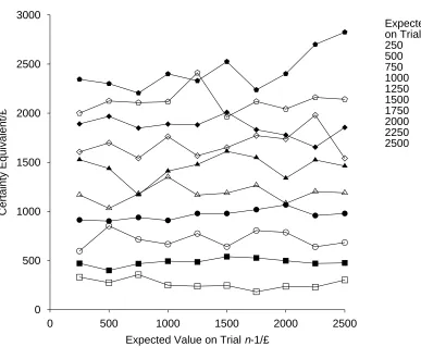
Figure 9 plots the mean value of prospects, as a function of the expected value of the
previous prospect, for each possible expected value of the current prospect. CEs given to a
prospect increased as the expected value of the prospect increased. The response was, on
average, 97% of the expected value (SD = 36%) showing slight risk aversion, on average. The
expected value of the previous prospect had no effect on the value assigned to the current
prospect (i.e., the lines in Figure 9 are flat).
To examine possible sequence effects more closely, we completed a linear regression
for each participant to see what proportion of the variability in the current response could be
explained by the previous prospect's expected value after the effects of the attributes of the
current prospect had been partialled out. The previous prospect's expected value was a
significant predictor of the current response for just 1 of the 14 participants, no more than
would be expected by chance. For this participant, r2 = .04, and for all other participants r2
< .04. Similar analyses for the previous (a) response, (b) x, and (c) p also showed no
sequential dependencies. (For this design, an r2 .08 can be detected with a power of 80%.)
Across all participants, the mean slope of the best fitting regression lines did not differ
significantly from zero for any predictor from the previous trial.
Discussion
In perceptual tasks where a series of stimuli are presented and a judgment is made after
each stimulus, the response to the current stimulus is shown to depend on the stimuli (or
responses; the two are normally highly correlated) on previous trials. In other words, the
response on the current trial is systematically biased by (some aspect of) the previous trial.
Some authors (e.g., Birnbaum, 1992) have suggested that judgments about risky prospects
dependencies like those shown in the analogous perceptual judgment tasks. There was little
carryover of information from one trial to the next. This finding is consistent with Mellers et
al.'s (1992) result, where the buying prices of a set of critical prospects were at most only
slightly influenced by the expected value of (previously encountered) filler prospects.
Experiment 4
Experiments 1 to 3 investigated the effect of context in CE judgment tasks. Careful
discussion by Luce (2000) highlighted the difference between judged CEs, where participants
provide a single judgment of the value of a prospect, and choice CEs, derived from a series of
choices between risky prospects and fixed amounts. For example, for the kinds of prospects
with large amounts and moderate probabilities used here, judged CEs are larger than choice
CEs (see, e.g., Bostic, Herrnstein, & Luce, 1990). The preference reversal phenomenon (see,
e.g., Lichtenstein & Slovic, 1971) is evidence that there is often a discrepancy between
choice-based and CE-choice-based methods of assessing utility (see also Tversky, Sattath, & Slovic, 1988).
Indeed, Luce went as far as to advocate developing separate theories for judged and choice
CEs.
Experiment 4 investigated context effects in a choice-based procedure rather than a
judged CE-based procedure. Participants made a single choice from a set of simple prospects
of the form "p chance of x" where the probability of winning was traded off against the
amount that could be won. The context was provided by manipulating the range of values of p
(and therefore of x) offered.
Method
Participants. Ninety-one undergraduate and postgraduate students from the University
of Warwick took part. Ages ranged from 18 to 40 years, with a mean age of 26 years. An
approximately equal number of male and female participants took part. None had previously
participated in any other experiment described in this article. Payment was determined by
Design. Participants were each offered a set of simple prospects of the form "p chance
of x." Within the set, the probability of winning and the win amount were traded off against
one another, and thus the choice was between a large probability of winning a small amount
through to a smaller probability of winning a larger amount. Ten prospects were used: "50%
chance of £50," "55% chance of £45," ..., "95% chance of £5."
If utility is assumed to be a simple power function of x, as is standardly assumed in
economics, with exponent - that is u(x) = x - the EU of each prospect can be calculated.7
Figure 10 plots utility as a function of the probability of winning p for different curvatures of
the utility function (values of . For a risk-neutral person ( = 1.0), for whom utility is
proportional to monetary value, the probability of winning for the prospect with the maximum
utility is p = .5. For a risk-averse person ( < 1.0), the prospect with maximum utility has a
larger probability of winning a smaller amount; the maximum falls at higher p for lower . The
key observation is that the prospect with maximum utility in the set is determined by the level
of risk aversion . Thus, a participant's choice of prospect can be mapped directly onto a
degree of risk aversion.
There were three between-participants conditions in the experiment. In the free-choice
condition, all 10 prospects were presented. In two other conditions, the choice of prospects
was limited to either the first or the second half of the prospects available in the free-choice
condition. In the more risky condition, the prospects ranged from a "50% chance of £50" to a
"70% chance of £30." In the less risky condition, the prospects ranged from a "75% chance of
£25" to a "95% chance of £5."
Procedure. Each participant was presented with a sheet listing a set of prospects. The
prospects were presented in an ordered table, with a row for each prospect and columns
headed "chance of winning" and "amount to win." Probabilities were presented as percentages.
Participants were asked to choose one prospect from the set to play. Before making their
prospect was played, and participants were paid according to its outcome, multiplied by an
experiment exchange rate (0.002).
Results
The results are displayed in Table 1. Blank cells indicate that the prospect was not
available for selection in that condition. Two hypotheses were tested. The first was that
participants are sensitive to the absolute values of prospect attributes and are unaffected by the
choice options. According to this hypothesis, in the restricted choice conditions, participants
should have chosen the prospect in the set that was nearest to the prospect they would have
chosen under free-choice conditions. For example, in the more risky condition, only 5
participants selected the prospect "70% chance of £30" (less risky prospects were not
available), but in the free-choice condition, 3 + 6 + 3 + 1 + 5 + 1 = 19 participants selected the
prospect "70% chance of £30" or one less risky. A 2 x 2 contingency table was constructed to
test the hypothesis that there was no difference in the proportion of people selecting the
prospect "70% chance of £30" or one less risky between the two conditions. The difference in
proportions was significant, Fisher's exact p = .0002. An analogous table was constructed to
test the difference between the less risky and free choice conditions. Again, the difference in
proportions was significant, Fisher's exact p = .0029. In conclusion, we can reject the
hypothesis that participants in the restricted-choice conditions chose the prospect in the set
nearest to the prospect they would have chosen under free-choice conditions and were
otherwise uninfluenced by the set of options.
The second hypothesis tested was that, although there may be some effect of the
choices available, there would still be some effect of the absolute magnitude of prospect
attributes. If so, we would expect a tendency for participants in the most risky condition to
choose the least risky prospect available and vice versa. However, if participants' choices were
determined solely by the set of available prospects, then the distribution of responses across
risky conditions. There was no significant difference, 2(4, N = 61) = 2.89, p = .5767. In other
words, there is no evidence that the absolute riskiness of a prospect had any influence on the
choices made in each of the restricted-choice conditions. For this chi-squared test, a difference
in J. Cohen's (1988) w = 0.45 - which corresponds to a 2(4) = 27.45 - can be detected with
80% power.
Discussion
Participants were asked to select a single prospect from a set to play. Within the set,
the probability of winning a prospect was reduced as the amount that could be won was
increased. Thus, each participant faced a choice between prospects offering small amounts
with high probability through to larger amounts with a lower probability. In the restricted
conditions, participants were offered only a subset of the prospects available. If participants'
preferences were unaffected by the set of options provided, they should simply have chosen
the prospect closest to the prospect they would select under free-choice conditions. However,
the distribution of choices differed significantly from those expected under this prediction.
Instead, the set of options available seemed to determine participants' preferences, and there
was no significant evidence that participants were sensitive to the absolute level of risk implicit
in a prospect. In conclusion, the level of risk aversion shown by a participant was shown here
to be a function of the set of prospects offered.
We know of only one other experiment where the effects of the context provided by
the choice set has been shown to affect the prospect chosen. In an unpublished study by
Payne, Bettman, and Simonson (reported in Simonson & Tversky, 1992), participants were
asked to make a choice between a pair of three-outcome prospects. Adding a third prospect
that was dominated by one of the original prospects but not the other significantly increased
the proportion of times the (original) dominating prospect was selected over the (original)
nondominating prospect. This effect has also been seen when making nonrisky decisions
a pen from a lesser known brandname increased the proportion of participants selecting the
famous brand pen and reduced the proportion selecting the $6 (see Simonson & Tversky,
1992, for this and other examples). The notion of trade-off contrast, where participants who
are assumed to have little knowledge about the trade-off between two properties, deduce what
the average trade-off is from the current or earlier choice sets, can account for this type of
data.
However, it is not immediately obvious how the notion of trade-off contrast might
account for the results of Experiment 4. Across both contexts, the trade-off between
probability and amount was constant (as the chance of winning the prospect was increased by
5%, the amount to win fell by £5). Instead, it seems that participants had no absolute grip of
the level of risk implicit in each prospect in the choice set and instead chose a prospect with
reference to its riskiness relative to the other prospects in the set. This demonstration of
prospect relativity in choice is consistent with that described in earlier experiments, where CE
judgments were used.
Experiment 5
Our final experiment was designed to investigate the extent to which a choice between
two prospects is affected by preceding context. Thus, this experiment mirrors Experiment 3,
but with actual choices rather than CE judgments. On each trial, participants chose between a
sure amount of money and a prospect offering a larger amount with a known probability. Let
us informally call a trial risky (or safe) to the degree that participants are expected to prefer
the risky prospect (or the sure amount of money). For example, we expected people to prefer
the risky prospect over the sure amount more often in (a) a "50% chance of £100" or £10 for
sure compared with (b) a "50% chance of £100" or £40 for sure. Half of the trials, the
common trials, were given to all participants and were designed so that the sure amount was
such that a typical, moderately risk-averse participant would be indifferent between the sure
were manipulated between participants. For half of the participants, the filler trials were
constructed so that only a very risk-averse individual would be indifferent to the sure amount
and the risky prospect. For these risky trials, most participants should have favored the risky
prospect. For the other half of the participants, the filler trials were constructed so that only
relatively risk-neutral participants would favor the risky prospect. For these safe trials, most
participants should have favored the sure amount. The intention was to assess whether the
riskiness of the filler trials would affect choices on the common trials. If participants
represented current prospects relative to previous prospects, then the common trials should
have seemed relatively safe if the filler trials were risky, and participants should have favored
the safe, sure amount. Conversely, if the filler trials were safe, then the common trials should
have seemed relatively risky, and participants should have favored the risky prospect.
Method
Participants. Thirty-five undergraduate and postgraduate students from the University
of Warwick took part in the experiment and were paid £5 for participating in this and three
other related experiments. Ages ranged from 18 to 30 years, with a mean of 22 years. Two
thirds of participants were female.
Design. Thirty-six trials were generated, each of which comprised a simple prospect of
the form "p chance of x" and an amount offered for certain. The amounts £100, £200, £300,
£400, £500, and £600 were crossed with the win probabilities of .1, .2, .4, .6, .8, and .9 to
give 36 prospects. Half of the trials were selected at random and consistently used to set the
context. For half of the participants, the fixed amount offered on these trials was low, and for
the other half of the participants, the fixed amount was high. The other half of the trials was
common to both groups, and the fixed amounts were at an intermediate level.
A sure amount was generated by using Equation 2.
y=x p
1
(2)
a hypothetical power law utility function, u(x) = x. = 1 for a risk-neutral person. Smaller
values of denote greater risk aversion. For each condition, six values of were used. The
values 0.50, 0.55, and 0.60 were used to generate sure amounts for the common trials. Risky
fillers were generated using the values 0.35, 0.40, and 0.45, which made the prospects on the
experimental trials seem comparatively unattractive. Safe fillers were generated using the
values of 0.65, 0.70, and 0.75. (For the population used in this experiment, we observed
values of in this range in an unpublished study from our laboratory. The values of were
deduced from choices between simple prospects and sure amounts.) The assignment of values
of to trials was such that a given value of occurred only once for each probability and only
once for each prospect amount. Otherwise, the assignment was random and the same for all
participants.
Procedure. Participants were given brief oral instructions. They were told that they
would have to imagine making choices between playing a prospect to receive an amount of
money and taking a smaller amount for sure. Each pair of options was presented on a separate
page of a 36-page booklet and appeared as follows:
Which option do you prefer?
10% chance of £300
£12
Participants were told to mark the option they would prefer and move on to the next
page. They were also made aware that there was no objective right answer and that choice
was a matter of personal preference.
Results
The dependent measure was the mean proportion of trials on which the prospect was
preferred to the sure amount. With safe fillers, participants selected the risky prospect
significantly more often in the experimental trials (mean = .53, SE = .04) than in the filler trials