Partitioning of Spatial Data in Publish Subscribe Messaging Systems

(1)

University of Twente

Master Thesis

Partitioning of Spatial Data in

Publish-Subscribe Messaging Systems

Author:

Rik van Outersterp

Supervisors:

dr. ir. M.J. van Sinderen

dr. R.B.N. Aly

dr. ir. N.C. Besseling

(2)

(3)

Abstract

A global trend to gather and query large amounts of data manifests itself more and more in our daily lives. This data includes that of spatial data, which increases the need for big data systems that can process this type of data efficiently regardless of preferences of end-users or the amount of data. The growing trend of big spatial data increases the need for expansion of knowledge about how such systems can be scaled up to satisfy both the increasing supply and demand of such data. Publish-subscribe messaging systems are capable of handling large amounts of data. Publishers send data to intermediary brokers, from which subscribers can retrieve the data. On these brokers data is stored in topics, which can be used to retrieve data efficiently based on a subscribers preferences. Topics can consist of multiple partitions in which the data is stored, which may improve load balancing and fault tolerance if multiple servers are used. A partitioning method defines in which partition data is stored on a broker. Partitioning of spatial data is a challenge, since spatial data is more complex than non-spatial data.

In this thesis we investigate how spatial partitioning methods can help to scale up publish-subscribe messaging systems for processing big spatial data. For this we present a case study consisting of Apache Kafka, an open-source publish-subscribe messaging system. In the case study the Kafka system processes road traffic data.

In our research we discuss existing spatial partitioning methods. We show how one of these, Voronoi, can improve processing of spatial data in a publish-subscribe system when compared to a system without spatial partitioning. In addition, we propose a new spatial partitioning method based on Geohash to overcome several drawbacks of Voronoi.

(4)

(5)

Introduction

1.1 Spatial data

Spatial data refers to objects in multidimensional space. These data objects can vary from a single point to a multidimensional polygon. When the space in which data is located is geographical, spatial data is often referred to as geospatial data. Examples of geospatial data are tweet messages of Twitter with the sender’s location, satellite images of the earth, or GPS data of cars on the highway.

Spatial data has some unique properties in comparison to non-spatial data [1], including the following.

Complex structure. Spatial data has a complex structure in which a data object can vary from a single point to a complex polygon in multiple dimensions, which usually cannot be stored efficiently in a traditional relational database.

Dynamic. Spatial data is often dynamic, because insertions and deletions are interleaved with up-dates of existing data, though this may not be specified within the insertion or deletion. Therefore structures that handle spatial data should support this behaviour without declining performance.

Open operators. Many spatial operators are not closed. This means that the outcome of

operations cannot be predicted beforehand, e.g. an intersection of two polygons can return any number of single points, dangling edges, or disjoint polygons.

Due to these properties, traditional data processing systems cannot process spatial data with similar efficiency as non-spatial data [1]. This problem holds especially for systems that process a large amount of data, i.e. big data systems based on techniques as Hadoop or MapReduce. These systems do not support these properties by default and for them the only way to process spatial data with more efficiency is to treat it as non-spatial data or to use handling functions for spatial data around these non-spatial systems. An example of a handling function is Geohash, a technique that hashes the latitude and longitude coordinates into a character string, such that it can be used as an indexing technique within a key-value environment.

However, both approaches treat spatial data as non-spatial data or use handling functions that do not take advantage of the properties of spatial data and therefore are not able to achieve the same efficiency that can be accomplished when processing non-spatial data. This is a growing problem, since a global trend to gather and query large amounts of data, including spatial data, manifests itself more and more in our daily lives. Examples of such uses are projection of spatial data on a visual map or calculation of an estimated time of arrival (ETA) for road traffic. These use cases are described in more detail in Section 2.3.

1.2 Big spatial data systems

To overcome the problem of less efficiency, extensions such as Hadoop-GIS and SpatialHadoop were developed. These systems are specialized in processing big spatial data and are capable of processing spatial data with similar efficiency as their traditional counterparts process non-spatial

(8)

6 Chapter 1. Introduction

data. They achieve this by focusing on how to process spatial data in an efficient way by improving partitioning and indexing techniques.

According to [2], a design for systems to handle big spatial data efficiently should consist of four main system components: language, indexing, query processing, and visualization. These components are described in more detail below and an example of such a system is visualized in Figure 1.1.

Language. A high level language allows non-technical users to interact with the system.

Indexing. Although it is referred to as the indexing component, it is not only responsible for indexing data, but also for partitioning data. Because partitioning and indexing are closely related, they are often used interchangeable in the literature. We define partitioning data as how data can be divided such that it is stored efficiently, and indexing data as organizing data such that it can be retrieved efficiently. For example, in a distributed environment a two-level structure can be used, where data is first partitioned across the machines, and then indexed locally on each machine.

Query processing. The query processing component consists of the spatial operations that are executed on the spatial data using the constructed spatial indexing and/or partitioning.

Visualization. Data output can be visualized by generating an image, such as a map or a graph.

Although [2] proposes that big spatial data systems should contain of all four components, we argue that effective scaling up of spatial data systems to big spatial data systems is dependent on only two of these components, namely the query processing and indexing components. Both components are responsible for processing data as efficiently as possible, while the other two com-ponents (language and visualization) are not necessarily required: systems can work without a high level language (although this might require trained users for interacting with the system) and query results do not always have to be visualized in an image, e.g. the previously mentioned use case of calculating an estimated time of arrival (ETA). Missing one or more of these components can also be seen in Hadoop-GIS. According to [3], Hadoop-GIS consists of only three of these components, namely the language, query processing, and indexing component.

Figure 1.1: (a) The indexing component is responsible for storing the input data into the database. (b) A user sends a request in a high level language. (c) The request in high level language is translated to a query. (d) Querying the database using the indexing component. (e) Query results are sent to be visualized. (f) A visualization of the results is returned to the user.

1.3 Publish-subscribe messaging systems

(9)

Chapter 1. Introduction 7

Publish-subscribe messaging systems use asynchronous communication as messages are tem-porarily stored on an intermediary message broker and not sent directly from publishers to sub-scribers. Because of this, a publish-subscribe messaging system is said to be a loosely coupled environment. A major advantage of a loosely coupled environment is its scalability: publishers and subscribers are completely unaware of each other’s existence and as they do not have to con-sider each other by keeping track of each other’s status, location, and preferences, the amount of publishers and subscribers can be higher than in peer-to-peer like systems. However, when publish-subscribe systems are scaled up towards large-scale sizes, their scalability will get limited by the message broker and its ability to handle large amounts of data.

Figure 1.2: Schematic view of publish-subscribe messaging systems.

1.4 Research problem & questions

From the previous sections the following can be concluded. Spatial data in itself has properties that makes it more difficult to process by traditional systems that do not take advantage of these properties, thus traditional systems process spatial data with less efficiency than non-spatial data. This really becomes a problem since there is a growing trend of gathering and processing big spatial data. For this data to be processed efficiently, big spatial data systems are developed, which aim to process spatial data as efficiently as traditional big data systems process traditional data. We argued that only two of the proposed main components for big spatial data systems are required in all cases for scaling up spatial data systems, namely the query processing and indexing components. An existing type of system that can handle big data and is scalable for growing data needs, is that of publish-subscribe messaging systems. However, these systems are originally not designed for big spatial data and it is therefore unclear how publish-subscribe systems can be scaled up in order to be able to process the growing amounts of big spatial data.

In this research we investigate if, and if so how, the upscaling of publish-subscribe messaging systems can be improved for big spatial data processing. We do this by applying a required com-ponent of big spatial data systems in a publish-subscribe messaging system. For this research we chose to apply only one of the most important components of big spatial data systems as a first contribution to the research field of spatial data in publish-subscribe messaging systems. We de-cided to limit our focus to the indexing component to investigate its effectiveness through a spatial partitioning method, because an optimized partitioning method improves the query performance and therefore the interaction with the system. Thus, we want to investigate if spatial partitioning can be applied to publish-subscribe messaging systems, and if so, which methods can be applied and how these perform in comparison to a system without spatial partitioning applied.

We formalize the research problem into the following research question as the objective for this research.

How can spatial partitioning methods help to scale up publish-subscribe messaging systems for pro-cessing big spatial data?

In order to provide an answer to this question, we first answer the following subquestions.

(10)

8 Chapter 1. Introduction

Publish-subscribe messaging systems and how spatial partitioning can be applied in them, are discussed in more detail in Chapter 3.

Which spatial partitioning methods exist that can be applied in publish-subscribe messaging sys-tems?

In Chapter 3 we present several spatial partitioning methods and discuss their applicability.

What is a suitable use case to evaluate applicable methods and how do these methods perform in this use case in comparison to a system without spatial partitioning?

In Chapter 2 we present a case study with multiple use cases for spatial data. One of these use cases is used in the experiments as described in Chapter 6. Models of the evaluated methods (Voronoi and Geohash) are described in Chapters 4 and 5.

Our research is intended to provide insight in how spatial partitioning methods can help to im-prove the scalability of publish-subscribe messaging systems in order to process big spatial data. As the amount of available spatial data increases, it increases the need for expansion of knowledge about how such systems can be scaled up to satisfy both the increasing supply and demand of this data. We provide this insight by investigating the applicability of an existing method and how it performs against a proposed spatial partitioning method called Geohash.

1.5 Outline

The outline of the thesis is as follows.

Chapter 2 presents a case study for this research that consists of a publish-subscribe messag-ing system. From this case study we define a suitable use case for the remainder of this research.

Chapter 3 discusses publish-subscribe messaging systems in more detail and how spatial partition-ing methods can be applied in these systems. In this chapter we also present several partitionpartition-ing methods.

Chapter 4 defines one of the presented spatial partitioning methods (Voronoi) in a model that is used in the experiments of this research.

Chapter 5 proposes a new spatial partitioning method based on Geohash. This method is de-fined in a model that is used in the experiments of this research.

Chapter 6 discusses the experiments of this research and found results.

(11)

Chapter 2

Case Study

This chapter presents the case study for this research. For this case study the Connect 2 system of Simacan is used. Simacan, a subsidiary of OVSoftware, is an IT company in the Netherlands that is specialized in gathering geospatial road traffic data and making it accessible and useful for its clients. In order to accomplish these goals, Simacan has developed several tools for its clients to access the gathered data in a user-friendly interface, e.g. easily readable traffic updates or visual representation of traffic on a map. For these products Simacan gathers roughly three types of geospatial traffic data:

• Traffic data per segment or measuring point. These data consists of traffic velocity, intensity, or incidents in predefined road segments or at road measuring points.

• Floating car data. These data consists of a single vehicle’s velocity, position, and direction.

• Other traffic related data. This includes weather information and charge points for electric or hybrid vehicles.

Currently, the focus of Simacan is the segment or measuring point traffic data, which is gathered from multiple public and private sources, including TomTom, the Dutch National Data Warehouse for Traffic Information (NDW), and the Dutch Ministry of Infrastructure and Environment (Rijk-swaterstaat).

Simacan aims to advance the functionality of its current system, Connect 1. Concrete examples of advanced functionality are storing data from a larger covered geographical area and from a larger time period (increasing the amount of historic data). Mainly due to the use of a relational database, the current system lacks the scalability capacity to achieve these aims: calculations made on the data would require to much resources and time to complete. Therefore they are limited to the scope of the Netherlands and a history of up to four hours back. They also aim at (a more advanced) support of routes, which can be defined by a client. In this scenario only relevant data regarding a defined route is pushed (in real-time) to the client, instead of, for example, publishing a list of all traffic related events in the Netherlands.

In their aim to achieve these goals a new system, Connect 2, is in development. In the next sections this system is described in detail.

2.1 Background

In this section we discuss several techniques that are used in Simacan’s Connect 2.

2.1.1 Apache Kafka

Apache Kafka, hereafter referred to as Kafka, is a publish-subscribe messaging system rethought as a distributed commit log [4]. It was originally developed by LinkedIn, but donated to Apache, although most developers of Kafka are still from LinkedIn.

The general concept of Kafka can be described as follows. Publishers send messages to one or more intermediary message brokers and subscribers can retrieve messages that are stored on this brokers. In Kafka publishers are called producers and subscribers are called consumers. Similar

(12)

10 Chapter 2. Case Study

to other publish-subscribe messaging systems, messages are categorized in topics. Each topic can consist of multiple partitions in which the messages are stored, see Figure 2.1. Compared to other messaging systems, Kafka consists of so-calleddumb brokers: they only store the messages and do not care who reads them (they also do not push the messages to consumers) or even who publish them for that matter.

Kafka runs on Apache ZooKeeper, an open-source server that includes various standard services in order to let Kafka be as simple as possible [5]. ZooKeeper can be used to configure Kafka and its components. It also keeps track of the state of all components within Kafka, e.g. which broker a replication leader is or which consumers are still alive and communicating with the cluster.

We will now describe each component of Kafka in more detail.

Producers. Producers publish messages to a topic. During this process, producers are respon-sible for choosing the partition on which a message needs to be be stored. By default this is determined by a hash-mod of a key, but producers can use a custom partitioning method. When such a key is not given, the message will be sent to a random partition. Because of the producers being responsible for choosing a partition for each message, they are responsible for load balancing messages to the various brokers, although this can only be achieved by a partitioning method that is designed for load balancing. It does not matter if a producer cannot see the corresponding broker initially: all brokers can be discovered by a producer from any single broker.

Producers have three levels of acknowledgement when sending messages to a broker. Requesting more acknowledgements improves the fault tolerance, but it also requires more communication and resources as messages are not dismissed after sending until enough acknowledges are received.

• No acknowledgement (0). This means that a producer cannot guarantee that messages are actually received by a broker.

• Acknowledgement from n replicas (1..n). In this case a producer can guarantee that a message will be received by 1..n brokers.

• Acknowledgement from all replicas (-1). This means that a producer can guarantee

that a message is stored on all brokers it should be stored on.

Consumers. Consumers subscribe to topics and process published messages from those topics that they pull from the brokers. Since the brokers are dumb, consumers have to maintain track of their state (offset) themselves, i.e. consumers have to know which messages they did read and which not. Consumers can be grouped into consumer groups. For consumers within a consumer group applies that a consumer group reads a message only once. Thus consumers divide the load by retrieving messages for the whole group.

Broker. A broker is a server in a Kafka cluster and stores messages that are published by producers. A machine can consist of multiple brokers. A Kafka broker is not the same as a usual message broker, because it does not send a message to the designated receiver: it remainsdumbby receiving a message, store it in the topic and partition it is told to, send a copy of the message when requested by a consumer, and delete the message after a certain time or to make space for new messages. A broker is responsible for persisting the messages for a configurable amount of time, but it is dependent on the disk capacity. Messages are stored in an append-only log. When producers send a message, a sequential write is performed by the broker for the new message. Analogue to this, a sequential read is performed to determine all messages that have to be send to a consumer from a certain offset. This is actually one of the key features of Kafka, as sequential reads may be faster than random reads, especially when stored in the page cache. Note that messages are not deleted when read by consumers: messages are stored by brokers for a configurable amount of time, and this only depends if there is enough disk space available.

(13)

Chapter 2. Case Study 11

used by consumers to maintain track of which messages they have read. The messages within a topic are not totally ordered, but messages within a partition are order on the time of arrival.

[image:13.595.130.434.215.368.2]

A disadvantage of Kafka is that the number of partitions cannot be easily changed, since they are determined when creating a topic. In addition, existing messages cannot be moved to a new partition where they may belong in a new partitioning method, leaving two options. The first option is that publishers send those messages again to the new partition, leaving it up to the consumer to handle any duplicates. This however raises not only the problem of how to handle duplicates, but also how many messages should be send again. Another option is to leave it completely to the consumers to use both partitioning methods for a while to retrieve messages from the old partition. Again, this raises the problem how long this situation is required before unnecessary messages are retrieved, let alone how these should be handled.

Figure 2.1: Anatomy of a topic.

Partitioning of the topics can have two major advantages:

• Load balancing. Using an equal partition size and distribution of the partitions over the brokers, load balancing can be optimized, especially when storing data. In this case, each broker has to store the same amount of data, which costs the same amount of disk writes, I/O transactions, RAM, and disk space.

• Predictability. Using an equal partition size and distribution of the partitions over the bro-kers, predictability in several areas can be improved. First and foremost is the predictability of the required storage per partition on a broker. Having equal sized partitions on brokers increases the ability to determine how long data can be stored on a broker. This can be use-ful when not only the latest data is requested, but also older (historical) data. Considering historical data it can increase storage efficiency, since no larger partition can exist that limits the time frame of historical data.

Secondly, the prediction of estimated data transfer improves. When a partition is accessed, all messages from a certain offset on that partition are sent. Any additional filtering on the messages is left to be handled by the subscriber. When the partitions have similar size, a subscriber can predict the amount of bandwidth and temporarily storage that is needed for the messages.

Replication. Partitions can be replicated on other brokers for fault tolerance. In that case a partition has one broker acting as the leader and zero or more brokers as followers, called replicas. The leader handles all read/write requests, while all replicas passively follow the leader’s actions. When a leader fails, one of the replicas will become leader through a selection process handled by ZooKeeper. It should be clear that for optimal fault tolerance the replicas exist on different physical machines.

(14)

[image:14.595.118.514.65.204.2]

(a) (b)

Figure 2.2: Examples of location referencing by TMC (a) and OpenLR (b) [6].

2.1.2 Location referencing

Location referencing is the process of describing a location [6]. The description of a location can vary from a single street name to a point given in 3-dimensional coordinates that is as accurate as possible. These examples already show that methods and precision can widely vary. Regarding geospatial traffic data GPS coordinates seems the way to go at first glance, but when a road segment must be described it shows some drawbacks. A single GPS coordinate on a crossing of roads does not give any information about which road it refers to, let alone the direction. In order to overcome these drawbacks, several methods are developed. In this section two of the most well-known methods are introduced: Traffic Message Channel and OpenLR.

Traffic Message Channel

Traffic Message Channel (TMC) is a widely used location reference method for traffic data [6]. It describes a road, traffic jam, or something else traffic related by giving a start and an end point. These points can be looked up in a TMC table, resulting in the exact location that is referenced.

Despite the simple nature of TMC, it has one major drawback. It is not possible to describe roads that are not in the TMC table, which limits the coverage to only those roads that are in the TMC table.

An example of TMC can be found in Figure 2.2a.

OpenLR

OpenLR is a location reference method for traffic data originally developed by TomTom before made available as an open source project [7]. The major advantage of OpenLR over TMC is that it does not need a table with indexed roads. Similar to TMC it describes a location using start and end points. However, OpenLR uses latitude and longitude for these points. Optionally it describes via-points, characteristics of the road between the points, and the length of the road between the points. Therefore it can describe every road in existence, including those not covered by TMC, which makes the coverage practically 100 percent.

The major advantage of OpenLR is also its major drawback. Due to its flexibility a location reference in OpenLR needs more bits than one in TMC, and translation from and to a record in OpenLR costs more computational power. In order to reduce the needed resources for handling OpenLR messages in our research, we limit the necessary data for determining the location of a message to the first location reference point. This is based on the fact that OpenLR messages describe road parts between road connections. Thus, if one would describe a route in OpenLR, they use a road segment completely from the beginning or not at all: it is not possible to start halfway.

(15)

2.1.3 Web Map Service (WMS)

Web Map Service (WMS) is a protocol for creating a map with georeferenced data from a geo-graphic information system (GIS) [8]. A WMS request consists of WMS parameters and and image parameters. WMS parameters include, for example, the WMS version, requested layers (roads, cities, rivers, etc.), and coordinates. Image parameters describe properties for the returned image, such as format (e.g. PNG, GIF or JPEG), width, and height. An example of a WMS request is shown in Listing 2.3. As can be obeserved, a WMS request is executed on top of HTTP. The (xmin, ymin) and (xmax, ymax) coordinates of the requested area’s bounding box are included in

the request. We refer to this bounding box as the WMS window that covers the requested area. In Listing 2.3 the coordinates are given in EPSG:900913, which is different to the more familiar WGS-84 latitude and longitude system. The supported coordinate systems may differ per WMS server.

Currently handling a WMS request is the only implemented method of the Connect 2 system.

GET /wms

?SERVICE=WMS &REQUEST=GetMap &VERSION= 1 . 3 . 0 &LAYERS= &STYLES=

&FORMAT=image / png &TRANSPARENT=true

&HEIGHT=256 &WIDTH=256

&REFRESHINTERVAL=60000

&ANTICACHE=0.06480319829190706−1464250087472−472 &DATAURL=h t t p :// e x a m p l e . com/ l o o k u p

&URL=h t t p :// e x a m p l e . com/wms

&LAYERCONTAINER=[ o b j e c t O b j e c t ] &VISIBLEINLOCATIONSUMMARY=true

&CRS=EPSG: 9 0 0 9 1 3

&BBOX= 3 1 3 0 8 6 . 0 6 7 8 5 6 0 8 1 9 4 , 6 8 8 7 8 9 3 . 4 9 2 8 3 3 8 , 4 6 9 6 2 9 . 1 0 1 7 8 4 1 2 2 9 , 7 0 4 4 4 3 6 . 5 2 6 7 6 1 8 4 HTTP/ 1 . 1

[image:15.595.156.412.488.652.2]

Listing 2.1: Example of WMS request.

Figure 2.3: WMS response example.

2.2 Connect 2

(16)

2.2.1 From source to Kafka

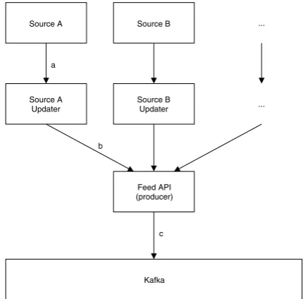
[image:16.595.205.424.114.326.2]

The process of data from a source to the Kafka cluster in shown in Figure 2.4.

Figure 2.4: Schematic overview of Connect 2, from source to Kafka.

Data from a source is sent to the Updater service corresponding with the source (a). Each source has its own road segment set that could change from day to day. The size and characteristics of these data sets differ per source, e.g. for the Netherlands TomTom has about 200.000 segments, while Rijkswaterstaat has less than 25.000 measuring points. For each road segment, that can have a length between a few tens of meters and a few kilometers, multiple properties are monitored, such as velocity, incidents, or intensity of the segment’s traffic. In general these properties are updated and published every minute, although this does not necessarily mean that Simacan retrieves a source’s complete data set every minute. Fortunately several sources have their own optimizations when it comes to sending updates and as a result the worst case scenario of retrieving all data sets in their entirety is practically never approached. For example, TomTom only sends the current velocity of a segment if the current velocity differs from a predefined default velocity when no special circumstances are applied, which is defined as the freeflow velocity.

The Updater service receives data from the source, performs some error handling and translates the received data into Simacan’s own standard format. This format is a JSON message, of which an example is shown in Listing 2.2. As shown, the complete message consists of the following fields.

• id The identifier of the message. Currently the encoded binary 64 string of the OpenLR data acts as the identifier.

• location The location reference in OpenLR encoded in a binary 64 string.

• feed The source of which the message originated.

• pub time src The time at which the message was published by the source.

• received time The time at which the message was received by the updater service.

• message The message related to the location reference, including data of what the speed at the location is, the location’s freeflow, the travel time over that segment, the quality of the provided travel time and speed as confidence, and if the road is blocked or not.

(17)

{

” i d ” : [ 1 0 0 , ”CwKUWCR5jRt8H/ubBbobEA==” ] ,

” l o c a t i o n ” : [ 2 0 0 0 0 , ”CwKUWCR5jRt8H/ubBbobEA==” ] , ” f e e d ” : [ 5 0 , ”tomtom−h d f l o w−dev ” ] ,

” p u b t i m e s r c ” : 1 4 5 6 4 0 7 6 9 0 0 0 0 , ” r e c e i v e d t i m e ” : 1 4 5 6 4 0 7 7 3 4 0 3 6 , ” m e s s a g e ” : [ 6 5 0 ,

{

” s p e e d ” : [ 1 0 0 0 0 , 7 6 ] , ” f r e e f l o w ” : [ 1 0 0 0 0 , 7 6 ] , ” t r a v e l t i m e ” : [ 3 0 0 0 1 , 8 7 ] , ” c o n f i d e n c e ” : [ 4 0 0 0 0 , 6 7 ] , ” r o a d B l o c k e d ” :f a l s e }]

}

Listing 2.2: Example of Simacan’s JSON message

2.2.2 From Kafka to client

[image:17.595.153.408.308.525.2]

The process of data from the Kafka cluster to a client in shown in Figure 2.5.

Figure 2.5: Schematic overview of Connect 2, from Kafka to client.

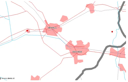
Data is continuously read from the Kafka brokers by a Map Server, which acts as a consumer in Kafka terms (d). The data that is received is immediately sent to the OpenLR Service (e). This service decodes the OpenLR data using the internal map, that is defined by map-links. The decoded data is visualized by the Map Server and kept in memory for two minutes. A client can sent a WMS request to the Map Server to retrieve the data. Since this data is the newest data available and generated not more than a couple of minutes before, Simican refers to this data as real-time data.

2.3 Use cases

Simacan has multiple use cases in which data currently is made available to its customers. As we shall see, these use cases can be divided into area or route based.

(18)

lower left corner and upper right are used to define this window. Currently only real-time data is visualized on a map, but also data from an earlier time (frame) can be visualized if the necessary methods for this are implemented on the consumer side.

Estimated Time of Arrival. When a route is defined, an estimated time of arrival (ETA) can be calculated. The difficulty in determining an ETA lies in the fact that the current situation on a part of the route may no longer apply by the time one reaches it. Therefore a combination of real-time data (data describing the current situation) and bought-in profile data (data that describes the usual traffic situation at a certain time based on historical data) is used when calculating the ETA.

[image:18.595.186.443.275.447.2]

Time-distance diagrams. In a time-distance diagram the traffic situation of a route is shown over a certain time. For example, on a route from A to B the average velocity of traffic is determined for every 1 kilometer for every 5 minutes. Each grid tile is then colored following a color scheme. The resulting image can be used by traffic experts to define the evolution of traffic jams or other traffic situations (Figure 2.6).

Figure 2.6: Example of a time-distance diagram that indicates two traffic jams [9].

Events in area and/or on route. Incoming events can be pushed to a client based on its route or area. These events can vary from traffic jam alerts to speed cams. Usually these messages come from different sources. Such event alerts are only useful when used real-time.

2.3.1 Conclusions

The use cases above show that there are multiple applications in which the collected traffic data is used. Each use case requests data from an area, a route, or a combination if a route is in multiple areas or multiple routes are in a single area. A possible future use case, in which data about a route and its surroundings is queried, also fits in this division as a combination of route and area based use case.

Although each use case also has a different time frame to request data from, this will not be considered in the remainder of this research. Historical or real-time are relative terms: all data is from the past and it is independent from the spatial partitioning from how far back the data needs to be retrieved.

(19)

Chapter 3

Spatial Partitioning in

Publish-Subscribe Messaging

Systems

In this chapter we discuss publish-subscribe messaging systems and what research has been done with regards to the application of spatial partitioning in such systems. Thereafter we present several existing spatial partitioning techniques. In these sections we provide an answer to how spatial partitioning can be applied in publish-subscribe messaging systems and which applicable methods already exist. The answer to these questions will be summarized at the end of this chapter.

3.1 Publish-subscribe messaging systems

When using multiple applications in a software environment, it may be necessary that applications have to communicate with each other. However, it is not practical for each application to have specified how to communicate with every other application. If that would be the case, many applications communicating with each other would end up in a so-called spaghetti architecture.

As a solution asynchronous communication consists of a loosely coupled environment in which applications send messages to an intermediary instead of directly to each other. One such environ-ment is a publish-subscribe messaging system [10], in which applications that create information publish messages and applications that are interested in that type of information subscribe to it, hence the name publish-subscribe. These types of applications are referred to as publishers and subscribers respectively. Messages are published to an intermediary message broker, which forwards the messages to subscribers, based on their subscriptions.

Two important types of publish-subscribe messaging systems are topic-based (also referred to as channel-based) and content-based. In topic-based publish-subscribe, messages are published to topics. Subscribers have subscriptions to one or more topics, receiving messages published to topics to which they subscribe. In content-based publish-subscribe, subscribers only receive messages if they apply to properties as defined by the subscriber. Because messages have to be queried against each subscriber’s properties, content-based costs more processing and resource usage than topic-based [11]. A hybrid of the two types is also possible; in such a system a subscriber only receives messages from topics it subscribes toand apply to properties as defined by the subscriber.

Publish-subscribe systems have two major advantages. As already mentioned, publish-subscribe is a loosely coupled environment. This means that publishers and subscribers are not aware of each other’s existence and can function without each other’s existence, unlike a tightly coupled environment such as a client-server architecture.

The second major advantage is that of scalability. Because the only communication publishers and subscribers have is with the intermediary broker, many publishers and subscribers can operate in the same environment. Communication can therefore be done in parallel and without updates about other nodes in the system, in contrast to systems in which a server needs to send updates about all clients to each client.

(20)

18 Chapter 3. Spatial Partitioning in Publish-Subscribe Messaging Systems

3.2 Spatial Publish Subscribe (SPS)

In [11] and [12] publish-subscribe for virtual environments (VEs) is discussed. In these environ-ments multiple nodes move within a virtual space while sending and/or receiving updates about the space around them, i.e. nodes can be subscribers, publishers, or both at the same time. For example, nodes are users in an online game who send updates about their actions and receive up-dates about actions of other users within their area of interest. [11] refers to these operations as the

event-process-update cycle: events are received by an intermediary that processes them and sends their results to nodes in the VE, whereafter new events are received and the cycle continues. This cycle can be executed in two ways: by spatial multicast or by spatial query. In spatial multicast messages are sent to nodes that are subscribed to an area within the VE. A node subscribes to an area of the VE when its area of interest overlaps with the area. In spatial multicast the VE is completely divided in multiple areas and therefore spatial multicast can be considered as the topic-based method. In spatial query nodes define properties which they query at times, e.g. the location of other nodes within its area of interest. Since these nodes only receive messages that apply to defined properties, this can be considered as the content-based method. A hybrid of the two approaches is possible as well, as presented by [13]. In this paper a model is presented for both spatial multicast (the spatial event model) and spatial query (the spatial subscription model). The spatial event model consists of the three most important aspects of a spatial event: who, when, and where. The spatial subscription model is used by subscribers to express their interest in spa-tial events, defined by i.a. a spaspa-tial predicate (within or distance). The hybrid between spaspa-tial multicast and spatial query is presented as a notification model that consists of a combination of the two other models.

Both spatial multicast and spatial query have their disadvantages. Implementation of spatial multicast faces the difficulty of finding the right area shape and size to divide the VE in. Further-more, spatial multicast sends messages to all nodes which have their area of interest overlapping with an area, regardless of the message actually being in their area of interest. Nodes will therefore need to spend time and resources filtering these irrelevant messages.

The major disadvantage of spatial query is that of its limited scalability. For n nodes that are required to answer a query, querying may takeO(logn) time [11], which limits the number of supportable nodes heavily. Furthermore, it may result in new nodes or updates not being queried or received fast enough.

In [11] and [12] it is argued that spatial multicast and spatial query do not satisfy basic require-ments for VEs on their own, but they do represent needed aspects of a complete system. Spatial Publish Subscribe (SPS) is presented as such a system that tackles the limitations of spatial query and spatial multicast, but can als support both methods. SPS provides nodes the ability to have both a subscription and a publication area, which is considered a subscription or publication point when the area’s size is 0. The intermediary message broker is referred to as an interest matcher, whose responsibilities are to record publication and subscription requests and to match published messages with subscriptions, sending the messages to the interested subscribers. Because of taking the area of interest into account in subscriptions, SPS is able to be more flexible and precise than spatial multicast. As for spatial query, a node in SPS does not need to query for updates as long as its subscription does not change.

3.3 Spatial partitioning methods

Although publish-subscribe systems such as SPS are designed for high scalability, supporting spatial publish-subscribe on a large-scale requires load distribution among the nodes. Since these nodes exist in a spatial environment, load distribution can be accomplished through partitioning of the spatial environment and its data, i.e. spatial partitioning. In SPS spatial partitioning is applied to the spatial environment in which the publishers and subscribers were located. However, it may not always be the case that publishers and subscribers have a spatial location themselves, and it may be that the data they send is spatial.

(21)

Chapter 3. Spatial Partitioning in Publish-Subscribe Messaging Systems 19

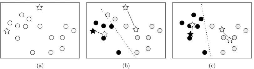
[image:21.595.79.485.67.177.2]

(a) (b) (c)

Figure 3.1: A space with two random added points as starting point of 2-means (a) and the first two repositions of these points (b and c). [14]

3.3.1 k-means

A partitioning method that is often referred to is k-means [14]. The idea of k-means is that data points within a multi-dimensional space are associated with the closest of theknewly added points. This association is accomplished as follows. In a space consisting of a number of points,k points are randomly added (Figure 3.1a). For every point in the space the nearest of these k points in determined (Figure 3.1b). Then thesekpoints are recalculated based on the points that are closest to them: thekpoints are placed in a spot where the distance between them and their associated points is the smallest (Figure 3.1b). Afterwards, for each point again the nearest of thek points is determined, which are calculated once more (Figure 3.1c). This process is repeated until the k

points do not acquire a new position to be placed at or after a predefined number of iterations. For the best possible outcome k-means is executed multiple times, each time with different starting locations of the k points. This requirement is therefore one of the major drawbacks of k-means: it does not guarantee that the optimal result that can be found using this method is actually found in practice, since it requires infinite executions to cover all possible starting locations forkrandom added points. Another disadvantage of k-means is that one cannot decide the location of thekrandom added points.

3.3.2 kd-tree

One of the most known partitioning methods is that of kd-tree [15]. The name of this method refers to two main properties of this method: the result of executing the kd-tree algorithm can be drawn as a tree and the kd-tree algorithm works similar regardless of the amount of dimensions

k. Although this thesis focuses only on spatial partitioning in two dimensions, it should be noted that despite kd-tree being able to work in higher dimensions, it only seems to work efficiently in the lower dimensions [16].

The idea of kd-tree is to split a space (node) that consists of data points into two subspaces (child nodes) in order to build a balancing tree in which every leaf node consists of a single data point. The general algorithm for this construction of a kd-tree fornpoints in ak-dimensional space (Figure 3.2a) works as follows, iterating over thekdimensions. In every dimension the median of the points in a node is determined and the node is split at the median (Figure 3.2b). Then for every child node the new median in the next dimension is determined and the node is split again (Figure 3.2c). This process is repeated until every node contains only a single point. Splitting at the median ensures that the resulting tree remains balanced.

We see that despite using both k in their name, the k in kd-tree refers to the number of dimensions, while thekin k-means refers to the number of newly added points. Another difference between the two algorithms is that kd-tree guarantees that the optimal result that can be found using this method is actually found. However, in order to guarantee this, kd-tree does need to be executed for all possible sequences of the dimensions. For example, in two dimensions this sequence can be either starting with division over the x-axis followed by division over the y-axis (as depicted in Figure 3.2) or starting with division over the y-axis followed by the division over the x-axis.

3.3.3 Voronoi

(22)

20 Chapter 3. Spatial Partitioning in Publish-Subscribe Messaging Systems

[image:22.595.250.380.515.618.2]

(a) (b) (c)

Figure 3.2: A two dimensional space (a) with the first two iterations of kd-tree (b and c). [16]

in VEs [11] and [12]. Due to the nodes being moveable in a VE, VSO is required to continuously adjust the cells of a Voronoi diagram in which the space of a VE is divided and in which the nodes move around.

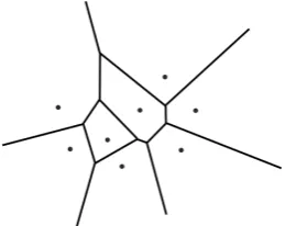
A Voronoi diagram, shown in Figure 3.3, is the result of Voronoi, a spatial partitioning method that divides space according to thenearest neighbour-rule: each point, called a site, is associated with the region that is closer to it than to all other points in the space [17]. This means that a Voronoi diagram requires a pre-defined set of sites, in which each site has their own region without any other sites. The regions are separated by an edge that is exactly on the equal Euclidean distance between two sites. Region on the boundary of the diagram may have an arbitrary infinite size if the divided space has no boundaries by itself. A vertex defines the location where three or more edges meet, and thus the Euclidean distances are equal between the corresponding three or more sites. Now it can be observed that a vertex is the center of a circle that touches at least three sites, but does not enclose any site: otherwise a vertex would be located elsewhere. In summary, a Voronoi diagram withnsites hasnregions that are separated by at most n₂edges, although the actual number of edges would be much lower when the number of sites increases [17]. When the number of sites is high, most of them would have multiple regions between them that hide their separating edge. The number of vertices is at most in the same order of vertices, but can also be none if all sites are located in a straight line.

Although we focus on two dimensional Voronoi diagrams in this research, it should be noted that, similar to k-means and kd-tree, Voronoi diagrams can be applied to multi-dimensional space, which would result in multi-dimensional regions.

Figure 3.3: Example of a Voronoi diagram with 8 sites [17].

(23)

Chapter 3. Spatial Partitioning in Publish-Subscribe Messaging Systems 21

3.4 Conclusions

In Section 3.1 we discussed publish-subscribe messaging systems. The two important advantages of publish-subscribe are the loosely coupled architecture and, partly because of that, scalability of these type of systems. Important to note is that in general publish-subscribe is either topic-based or content-based.

We then presented a publish-subscribe mechanism for spatial virtual environments called Spatial Publish Subscribe (SPS) in Section 3.2. In SPS nodes can be both publisher and subscriber which communicate with an interest matcher. However, being able to support SPS on large-scale, load distribution is necessary. This can be achieved by dividing the nodes over multiple interest matchers. Since this partitioning takes place over nodes in a space, this is referred to as spatial partitioning.

Before we presented several spatial partitioning methods in Section 3.3, we argued that the way that spatial partitioning is used in SPS may not be applicable to other publish-subscribe systems, as it is not always the case that subscribers and publishers have a spatial location: it may also be in the data itself.

(24)

(25)

Chapter 4

Voronoi Model

In Section 3.3.3 we presented Voronoi as a spatial partitioning method. In this chapter we describe how a Voronoi diagram can be constructed and how Voronoi can be applied as a spatial partitioning method in a publish-subscribe messaging system.

4.1 Construction of a Voronoi diagram

In this section we present three algorithms that are used for the construction of Voronoi diagrams. Recall from Section 3.3.3 that the construction of a Voronoi diagram requires a given set of points that are referred to as Voronoi sites.

4.1.1 Fortune’s algorithm

Fortune’s algorithm is a sweep line algorithm in which a straight sweep line L sweeps over the Voronoi sitesS in one direction [19]. When a sites∈S is passed byL, a beach lineB defines the line on which every point is equidistant to both L and the passed site, as shown in Figure 4.1a. Because Lis a straight line, B results in a parabolic curve. Where beach lines of two sites meet, a Voronoi edge is created as the Euclidean distance between each site and this meeting point is equal (Figure 4.1b). Note that any sites that are not yet passed byLdo not affect points that are passed byL.

(a) (b)

Figure 4.1: Illustration of Fortune’s algorithm for one site (a) and multiple sites (b) [20]. The beach lineB marks all points that have an equal distancedto the Voronoi site and sweep lineL.

4.1.2 Lloyd’s algorithm

In Lloyd’s algorithm a Voronoi diagram is created in a space such that each site is located at the center of its Voronoi cell [21]. The algorithm shows some similarities to k-means, which was described in Section 3.3.1. Lloyd’s algorithm starts with k sites in a space. For these k sites a Voronoi diagram is constructed (Figure 4.2a). Then for each Voronoi cell the center is determined and allksites are moved to the center of their cell. Then a new Voronoi diagram is constructed using the new locations of the k sites (Figure 4.2b), after which the center of each cell is determined,

(26)

24 Chapter 4. Voronoi Model

and so on. This process is repeated until each site is located at the center of its Voronoi cell (Figure 4.2c).

[image:26.595.131.517.511.652.2]

(a) (b) (c)

Figure 4.2: A two-dimensional space is divided in a Voronoi diagram (a). Each site is relocated to the center of its cell, resulting in a new Voronoi diagram (b). This is repeated until all sites are located on the center of their cell [22].

A clear difference to Fortune’s algorithm is that Lloyd’s algorithm can only be used if the positions of the Voronoi sites are not of any interest. This can be argued as either a drawback or an advantage, based on the requirements for Voronoi diagram. However, a clear drawback in comparison to Fortune’s algorithm is that Lloyd’s algorithm needs multiple iterations to achieve its purpose and each iteration a new Voronoi diagram is constructed.

4.1.3 Delaunay trangulation

A Voronoi diagram is the dual of a Delaunay triangulation [23]. Therefore, a Delaunay triangulation can be used to construct a Voronoi diagram. In geometry, a Delaunay triangulation is a type of triangulation, which is a planar object that is divided into triangles. A Delaunay triangulation contains a set of points P such that no points exist within the circumcircle of any triangle in the object (Figure 4.3a). A Voronoi diagram of P is constructed by determining the centers of the circumcircles of all triangles (Figure 4.3b). The centers are then connected with each other such that they include exactly one pointp∈P in each region they form. The connections between the centers are the edges of the Voronoi diagram, with the centers being the vertices (Figure 4.3c).

(a) (b) (c)

Figure 4.3: Construction of a Voronoi diagram from a Delaunay triangulation. Given a Delaunay triangulation (a) the centers of all circumcircles are determined (b). The centers are the vertices in the Voronoi diagram (c). Only four of the twelve circumcircles and centers are shown [23].

4.2 Voronoi spatial partitioning algorithm

(27)

Chapter 4. Voronoi Model 25

For a data message it determines the nearest site by calculating the Euclidean distance between the message’s location, which in our research is defined by the first location reference point in a message as discussed in Section 2.1.2, and each site. In terms of time complexity, this algorithm is O(n). The message is then sent to the partition corresponding to the nearest site. Listing 4.1 shows our partitioning algorithm.

Set<S i t e> s e t O f S i t e s ; // s e t o f a l l s i t e s i n Voronoi diagram

S i t e l o c a t i o n ; // l o c a t i o n from message

S i t e currentNN ; // c u r r e n t n e a r e s t n e i g h b o u r

currentNN . C o o r d i n a t e s = (MAX, MAX) ;

foreach ( S i t e s i n s e t O f S i t e s )

i f d i s t a n c e ( l o c a t i o n , s ) < d i s t a n c e ( l o c a t i o n , currentNN ) currentNN = s ;

Listing 4.1: Pseudo code producer inO(n)

Application of WMS requests

In Section 2.3.1 we decided to use the use case of WMS requests for our experiments to measure the performance of spatial partitioning methods. WMS requests can be handled by a subscriber in the Voronoi model as follows. Recall from Section 2.1.3 that a WMS request defines a square window that is defined by four pairs of latitude and longitude coordinates. In order to call the correct partitions, it is required to calculate which partitions overlap with the requested window. Due to the irregular shapes of the Voronoi cells, the only approach to do this is by spatial intersection. For this the window is compared to each Voronoi cell and returns true if it overlaps. Since all messages have to be retrieved from a partition, the shape and size of the overlapping is not required.

Figure 4.4 shows the process wherein overlap between the WMS request window and partitions is illustrated (Figure 4.4a), resulting in the partitions from which messages need to be retrieved (Figure 4.4b). The received messages are then filtered such that only the relevant messages remain, resulting in an image of the requested area (Figure 4.4c).

The process described shows that it is necessary for the subscriber to know the layout of the Voronoi diagram. During our experiments our subscriber used an open-source Java library based on Llyoyd’s algorithm [24]. In this library a Voronoi diagram is computed using a Voronoi power diagram, as described in [25]. In a power diagram a Voronoi site has a weight that influences the size of its cell. By setting these weights to 0 for all sites, an ordinary Voronoi diagram is constructed since sites are not pulled towards the center of their cell. Thus only one iteration of Lloyd’s algorithm is performed when constructing the Voronoi diagram.

(28)

(29)

Chapter 5

Geohash Model

In this chapter we propose Geohash as a spatial partitioning method. Geohash is a technique that hashes a location’s latitude and longitude coordinates into a single text string. This technique can be visualized as dividing the surface of the Earth into separate planes, i.e. spatial partitioning of Earth’s surface. To our knowledge, despite this approach no research has been done on the application of Geohash as a spatial partitioning method. In this chapter we describe Geohash in detail, how it can be applied as a spatial partitioning method, and what its main differences are compared to Voronoi and other spatial partitioning methods.

5.1 Geohash

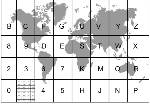
[image:29.595.131.431.474.681.2]

Geohash is a technique that allows a pair of geographical coordinates to be encoded into a single text string, called a geohash [26]. It was put in the public domain by Gustavo Niemeyer in February 2008 [27] [28]. The objective of Geohash is to have short strings of locations on Earth that can be used in URLs. This is accomplished by processing the latitude and longitude bitwise in base 32. Details of this process and the other way around are discussed in Sections 5.2 and 5.3. It is important to note that withGeohashwe refer to the technique of encoding a coordinate pair into a single string, whilegeohash refers to this string that represents the encoding of a coordinate pair.

Figure 5.1: Geohash example

Geohash can be visualized as a division of Earth into 32 planes, each of which can be divided again into 32 planes, and so on. Each plane is associated with a unique geohash and each division results in an additional character for its string. Figure 5.1 shows this division, where a second division is shown in the plane associated with geohash 1. We refer to these divisions as Geohash levels by defining level x the division that results in geohashes of length x. In short, we use

(30)

28 Chapter 5. Geohash Model

Geohash-x to define the level that consists of geohashes of length x. Thus, Figure 5.1 shows Geohash-1 and a part of Geohash-2. We define an implementation with geohashes of a shorter length as a lower Geohash level. For example, the highest Geohash level that consists of a geohash that covers the Netherlands in its entirety, describes therefore the longest geohash that completely covers the Netherlands (namely u1). Lower Geohash levels, and therefore shorter geohashes, would have the same results in our experiments since they consist of the same amount of geohashes when it comes to covering the Netherlands (namely one), while higher Geohash levels, and therefore longer geohashes, covers only parts of the Netherlands.

Although there is no official maximum (one can make a string as precise as they desire), in practice, including the official website geohash.org [29], usually a maximum of 12 characters is used, which results in an area of 3,7 by 1,9 cm around the equator, see Table 5.1.

Length of geohash Width Height 1 5.009,4 km 4.992,6 km 2 1.252,3 km 624,1 km 3 156,5 km 156,0 km 4 39,1 km 19,5 km

5 4,9 km 4,9 km

6 1,2 km 609,4 m

7 152,9 m 152,4 m

8 38,2 m 19,0 m

9 4,8 m 4,8 m

10 1,2 m 59,5 cm

11 14,9 cm 14,9 cm 12 3,7 cm 1,9 cm

Table 5.1: Approximate area size of a plane around the equator corresponding to a geohash of a certain character length [30].

This approach of Geohash can be used to define bounding boxes around spatial objects, a technique that can be easily applied to current systems without any modifications to their internal structure, since its resulting hash can be used as a key in a key-value system. As a result Geohash supports efficient updating, because no costly data structures such as trees or Voronoi diagrams are used.

Another advantage of Geohash emerge from the fact that spatial partitioning methods as Voronoi need (pre-defined) data points to divide an area, and those data points can be argued over. Geohash does not require any data apart from the area, i.e. Geohash is independent of any data set. This has as advantage that an area can be divided before any data is known.

In addition, because of Geohash hashing technique, it can be used as a simple and highly efficient filtering technique based on the prefixes in the hashes. When prefixes of hashes are common, the locations that those hashes represent are geographically close to each other as well. However, it is not guaranteed that locations that are close to each other result share a common prefix in their hashes. This drawback of Geohash can be illustrated by the following problems [31].

• Edge-Case Problem. Locations that are located on opposite sides of a covered area are close to each other geographically, but do not have a common prefix. It should be noted that this problem only appears in case of an area that is continuously at the edges. E.g. points in the far west and the far east when covering earth, (Figure 5.2).

• Z-Order Problem. Due to the Z-order traversal in which Geohashes are stored, points can be stored close to each other while not being close to each other geographically, or vice versa. E.g. areas 7 and 8 in Figure 5.3 are stored close to each other despite being geographically far from each other, while areas 7 and E are close to each other geographically but not in storage.

(31)

Chapter 5. Geohash Model 29

are usually stored on receiving time and not in another, location dependent index. The Edge-Case Problem may still exist in the design of our experiments, but does not play a role in our research due of the scope of our experiments being limited to the Netherlands, thus the covered area is not continuously at the edges.

Figure 5.2: Visualization of the Edge-Case Problem of Geohash.

Figure 5.3: Visualization of the Z-Order Problem of Geohash [31].

5.2 Encoding algorithm

The Geohash encoding algorithm constructs a geohash from a pair of latitude and longitude co-ordinates. The base 32 character mapping that is used for encoding and decoding is shown in Table 5.2.

Decimal 0 1 2 3 4 5 6 7 8 9 10 11 12 13 14 15 Base 32 0 1 2 3 4 5 6 7 8 9 b c d e f g Decimal 16 17 18 19 20 21 22 23 24 25 26 27 28 29 30 31 Base 32 h j k m n p q r s t u v w x y z

Table 5.2: Base 32 character mapping, used for encoding and decoding of geohashes.

The idea behind the encoding algorithm is that the longitude and latitude coordinates are used alternately to define the bits that make up a character, starting with the longitude coordinate. Since base 32 is used, five bits are required for each character. During execution of the algorithm the interval in which the coordinates is located is reduced. The more iterations are executed, the more precise the interval is, resulting more bits and thus more characters (i.e. a longer string).

(32)

The algorithm works as follows. Remember that we start with the longitude coordinate. When all steps are completed, the next iteration will be executed with the latitude coordinate, and so on.

1. The first step is to determine the middle value of the current interval.

2. If the current coordinate value is higher than the middle, a bitwise inclusive OR is executed between the current character bitschandbits[b], wherebits= 16,8,4,2,1. The result of this execution is stored in ch.

3. The current interval is changed to the half in which the coordinate value is included.

4. If we have not yet done five iterations of this algorithm, i.e. b < 4, the value of b will be increased by 1. Otherwise the value ofchdefines a base 32 character, which is added at the end of the current geohash. Both the values ofb andchare set to 0 afterwards.

The used implementation of this algorithm in Java can be found in the encode() method in Appendix A.

Example. Suppose we have the following longitude/latitude coordinates: lon= 6.851656 and

lat= 52.244048. As described above, we set the character bitschand current bitbto 0: ch=b= 0. The current coordinate intervals are lonInt = (−180,180) and latInt = (−90,90) for longitude and latitude respectively. We now show the first two iterations of the algorithm.

Iteration 0

1. Define middle midof current intervallonInt= (−180,180): mid= 0. 2. It holds thatlon > midsince 6.851656>0, thusch|bits[b] = 0|16 = 16.

3. Sincelon > mid, we change the current interval to the higher half: lonInt= (0,180)

4. We increase the current bit: b= 1.

Iteration 1

1. Define middle midof current intervallatInt= (−90,90): mid= 0. 2. It holds thatlat > midsince 52.244048>0, thusch|bits[b] = 16|8 = 24.

3. Sincelat > mid, we change the current interval to the higher half: latInt= (0,90)

4. We increase the current bit: b= 2.

We leave it up to the reader to show that the first character will be u, and the geohash can be calculated tou1kc5ytpxhmj.

5.3 Decoding algorithm

Similar to the enconding algorithm of Geohash as described in Section 5.2, base 32 is used for decoding geohashes into latitude and longitude coordinates. The base 32 character that is used can be found in Table 5.2.

(33)

Chapter 5. Geohash Model 31

1. Take the first bit. If low (0), set the lower half of the current interval as the new interval. If high (1), set the higher half of the interval as the new interval. E.g. if 1 is the first latitude bit, (0,90) is the next interval.

2. Repeat for every bit.

The implementation of this algorithm can be found in thedecode() method in Appendix A.

Example. Suppose we have the following geohash: u1kc5ytpxhmj. As described above, we set the current coordinate intervals tolonInt= (−180,180) andlatInt= (−90,90) for longitude and latitude respectively. Then we rewrite the geohash using Table 5.2 and number the resulting bits. The resulting bit sequence and numbering can be found in Table 5.3.

Base 32 u 1 k ...

Decimal 26 1 18 ...

Bits 1 1 0 1 0 0 0 0 0 1 1 0 0 1 0 ... Bit # 0 1 2 3 4 5 6 7 8 9 10 11 12 13 14 ...

Table 5.3: Decoding of first three characters of the geohashu1kc5ytpxhmj.

Recall that the even numbered bits belong to the longitude coordinate and all odd numbered bits belong to the latitude coordinate. We now show the first five iterations for each coordinate.

Longitude bits: 10000, which starting intervallonInt= (−180,180).

1. The first bit is 1, so we change the interval to the higher half of the current interval: lonInt= (0,180).

2. The next bit is 0, so now we change the interval to the lower half of the current interval:

lonInt= (0,90).

3. Again, the next bit is 0, thus: lonInt= (0,45).

4. Again, the next bit is 0, thus: lonInt= (0,22.5).

5. Again, the next bit is 0, thus: lonInt= (0,11.25).

Latitude bits: 11001, which starting intervallatInt= (−90,90).

1. The first bit is 1, so we change the interval to the higher half of the current interval: latInt= (0,90).

2. The next bit is 1 again, thus: latInt= (45,90).

3. The next bit is 0, so now we change the interval to the lower half of the current interval::

latInt= (45,67.5).

4. The next bit is 0 again, thus: latInt= (45,56.25).

5. The next bit is a 1, thus: latInt= (50.625,56.25).

We leave it up to the reader to show that the geographical coordinates of the geohash will be 6.851656 longitude and 52.244048 latitude.

5.4 Geohash applied as a spatial partitioning method

(34)

5.4.1 Spatial partitioning method application

The first step of applying Geohash as a spatial partitioning method is to define the geohashes that cover the area, e.g. by calculating the geohashes of the areas outer borders and filling up the geohashes inbetween. Depending on the exact calculation to define the area’s geohashes, duplicate geohashes may result. Therefore, the resulting list of geohashes should be filtered such that only unique geohashes remain with a given length. This amount of geohashes will be equal to the amount of partitions and each geohash is associated with exactly one partition. This association is stored in a list. Now the publisher and subscriber determine partitions as follows. They calculate a geohash from the given coordinates using the encoding algorithm described in Section 5.2. Then the resulting geohash is looked up in the list of association between geohashes and partitions to retrieve the associated partition.

Application of WMS requests

In Section 2.3.1 we decided to use the use case of WMS requests for our experiments to measure the performance of spatial partitioning methods. WMS requests can be handled in the Geohash model as follows. Recall from Section 2.1.3 that a WMS request defines a square window that can be defined by four pairs of latitude and longitude coordinates. In order to call the correct partitions, it is required to calculate which partitions (or geohashes) overlap with the requested window. Because both the window and the visualization of the partitions are rectangular shapes, there are two approaches by which the correct partitions can be determined. Both approaches make use of the structured way geohashes are created and do not require an expensive spatial intersect as used by Voronoi.

Figure 5.4: The process of selecting the required Geohash partitions for a WMS request, resulting in an image of the requested area.

The first approach is to use a matrix structure. Using this approach one could start in any corner of the WMS window and walk through the matrix to the point diagonal of it via the two neighbouring points. For example, in our implementation we started at the left upper corner of the WMS window and walked down and right through the matrix until we found the bottom left corner and upper right corner respectively. Then we walked right and down respectively until we found the bottom right corner. Afterwards, the geohashes in between are added, e.g. by a floodfill algorithm.

The second approach is to calculate the geohashes of each corner and the geohashes in between using the structure of geohashes. This works similar to the approach above, but it calculates geohashes on-the-fly instead of using a memory costly structure. For example, one could start with the upper left corner and work towards the upper right corner until it finds the geohash of the given pair of latitude and longitude coordinates. It then does the same for the row below, until it finds the geohashes of the bottom corners.

Partitioning of Spatial Data in Publish Subscribe Messaging Systems

University of Twente

Master Thesis