Optimizing the material flow at Bosch : supplying the Deventer plant with materials for making heating boilers

(1)

Optimizing the material flow at Bosch

Supplying the Deventer plant with materials for making heating boilers

Graduation Thesis

Anton Dijkstra, BSc

Supervisors:

Prof.dr. J.L. Hurink M.J. Brouwer

Dr. J.W.C. van Ommeren K. van der Rijst

(2)

(3)

3

Preface

With this thesis I finish my master Applied Mathematics at the University of Twente. The last 9 months I have worked at Bosch in Deventer with much pleasure. At the beginning of this assignment, the goal was vague: Improve and simplify the current situation with some kind of mathematical model. During the 9 month period, more restrictions became apparent. Wishes and other improvements were constantly suggested, which resulted in a model that changed continuously.

Next to making a model to describe the situation at Bosch, I have learned to program it in Virtual Basic for Applications, which was new for me. Thanks to this new learned skill, the model could be tested with historical data. I am very proud of the final version of this model and of the results that it produced. It was a big bonus for me that my model was implemented at Bosch. This meant that I not only had to pitch my ideas to the highest bosses at the

Deventer plant to convince them of the success of this model, but also that I had the chance to implement my own ideas. This was a great experience for me.

During my study, I always had affection with the world of logistics. This resulted in a minor Production and Logistic Management and many courses in my master about Industrial Engineering and Management. This graduation assignment was a perfect mix between

logistics and mathematics. It was a real world example of applying mathematics. All the time people ask me what I want to do when I am done studying. Thanks to among others this assignment, I found out that I want to go in the logistic world.

I want to give many thanks to my coworkers at Bosch, which treated me as a worthy

colleague. A special thanks goes out to my supervisors at Bosch: Maarten Brouwer, Koos van der Rijst and Marc Weulink. Next to that, I want to thank Johann Hurink for supervising my graduation, especially with reviewing my thesis. I know that I gave him a hard time

(4)

4

1. Introduction

This thesis describes the case of supplying the production process of one of the leading manufacturers of heating boilers in the Netherlands. The materials for the heating boilers are provided by multiple suppliers. These wholesalers supply the manufacturer by truck, which causes a large number of trucks delivering materials to the factory. These trucks cannot arrive at the same time, due to the limited capacity at the factory to unload the trucks. This means that the arrival times of all the trucks have to be adjusted to each other. At the same time, it has to be guaranteed that the production does not get to a standstill, due to the fact that the materials for production are not present at the time they are needed. To prevent this, coordination is needed between the arrival times of the trucks and the composition of the corresponding orders. In this thesis a model is developed which coordinates the determination of the arrival times of the trucks and the composition of the orders.

In the following more details on the manufacturer are given and the concrete setting of the relevant case is explained in more detail. Next to a description of the current situation at the manufacturer, both sub problems, the composition of the orders as well as the determination of the arrival times of the trucks, are elaborated. The subsection ends with a more detailed problem statement for this thesis. After that, background information is given about the way how the orders are composed within the considered factory. The system used for the

composition of the orders creates a link between the materials that are used in the production of the heating boilers and the materials that are ordered. This is done in a way that the

production does not come to a standstill. The section ends with an overview on how the remainder of the thesis is built up.

1.1. The manufacturer

The manufacturer of heating boilers on which this case is based is Bosch. This manufacturer has many divisions, each of which produces different products from laundry machines and screen wipers to heating boilers. The division Bosch Thermotechnology (TT) is responsible for the latter. This division has the mission to design and produce energy efficient solutions for heating, cooling and hot water. To achieve this mission, Bosch TT produces heating systems, heat pumps, commercial boilers, air conditioning and ventilation systems, solar thermal systems, domestic hot water heaters and more. Hereby, Bosch TT produces under different brands; Bosch, Buderus, Junkers, Vulcano, Worchester, e.l.m. LeBlanc, Dalkon, IVT and Nefit.

Bosch TT has over 20 production sites over the whole world, from which 16 are in Europe. At the Bosch production plant in Deventer heating boilers are assembled. The materials needed for this assembly are coming from The Netherlands, Germany, Turkey, some other European countries and Asia.

The predecessor of Bosch TT in Deventer, Nefit, was the first to launch a central heating boiler with high efficiency, the Nefit Turbo. In 1992, Nefit and Fasto B.V. went on together to get a better focus on the market and in 1997 half of the shares were sold to Buderus

(7)

7

1.2. Problem description

In this subsection the case of supplying the Bosch TT division in Deventer with materials is described in more detail. First an introduction is given of the current processes at the Deventer plant. Then, the problem of supplying the factory is described in more detail. This leads to the problem statement.

At the Bosch TT plant in Deventer the production of heating boilers is done following a “just in time” management. Just in time management is a type of production where commodities are only produced when there is a demand for that type of commodity. This means that the materials are ordered dependent on which commodities are produced. A consequence of the just in time management is that the inventory level of materials as well as finished goods is low. This reduces space and holding costs. A disadvantage of just in time management is that a small disruption in the delivery of the materials could cause a standstill in production. To prevent this, a good coordination between Bosch, the suppliers and the transport company HSL is required. The latter delivers the materials from the different suppliers to the Deventer plant.

Currently, the material flow is arranged such that the materials of the suppliers are stored at a local depot of HSL. This transport company delivers the material regularly to the Deventer plant. To optimize this material flow a system called Milkrun is going to be used. The

Milkrun system consists of an order part and a delivery part. An order consisting of materials that were just used for the production of heating boilers is send to the supplier. This is done following the just in time philosophy. The supplier needs time to process the order and pick the materials such that a truck from HSL can transport those materials directly to the Deventer plant. When those materials are delivered and unloaded from the truck, the materials are used for the productions of new heating boilers and the cycle starts over again.

The choice for the Milkrun system makes determining the arrival times of the trucks of HSL a complex task. The reason for this is that in the whole supply chain the inventory level is low, which means it is more critical that the trucks deliver the materials on time in order to prevent a standstill in production. A restriction that makes this even more complicated is the fact that at the Deventer plant, there is only one dock to load and unload materials. This means that only one truck can arrive at a time. Next to that, unloading the trucks takes some time such that the unloading of the next truck can start only after that the unloading of the previous truck has been completely finished. One of the goals of the model developed in this thesis is to automatically determine when the trucks must deliver their materials to the Deventer plant.

Next to the most crucial restriction of having only one dock, there are some other restrictions which are described in the next section. In the following, some more details about the problem of supplying the Deventer plant are given which are needed to formulate the problem

(8)

8

First, the structure of the orders is explained. An order consists of materials that were just used in the production of heating boilers. Due to the just in time management, this relates directly to the demand of heating boilers. The demand consists of long-term customer orders and short-term customer orders. The long-term customer orders create the season pattern, but do not change often. The short-term customer orders come in a week in advance and causes that the demand for heating boilers changes every week. As a consequence, the amount of materials needed for the heating boilers also changes every week. Due to this and the just in time management, the orders differ every time.

An order consists of a list with all the materials that have to be delivered and the amount that is needed per material. These amounts have to be such that the total order can be delivered by one truck. This means that all the amounts of material together must not exceed the capacity of the truck. This can be regulated by choosing the moments that the order is send to the supplier. For this is assumed that all the materials that are on the current order are those that are used in production from the moment that the previous order is send until the moment the current order is send. By regulating these moments, the composition of the orders can be established. Concrete, a Kanban system is used to implement this strategy. In section 1.3 more details are given about this system.

Before going into more detail about the problems with the delivery, a small note has to be made. There is a difference between two types of materials: Small volume materials and great volume materials. The great volume materials are produced by suppliers nearby and are transported by HSL directly from the suppliers to the Deventer plant. The other (small volume) materials are gathered, stored and delivered to the Deventer plant by another

transporting company called Veenstra. The trucks that deliver small volume materials are not regarded in this model, but their schedule is considered as input for this model. The reason for this is that the schedule for these trucks is more or less the same every week and that in the nearby future the whole operation regarding small volume materials is going to change, such that scheduling those trucks would become useless.

The most crucial problem with the delivery is that there is only one dock to unload the trucks as discussed at the beginning of this section. Next to that, the impact of the changing demand on the trucks of HSL is great. Those trucks usually deliver six to seven times a day to the Deventer plant, but that can increase to ten times a day. Furthermore, trucks from Veenstra deliver five times a day. Those trucks deliver the small volume materials at fixed times to the Deventer plant. This is not the case for the trucks of HSL. Moreover, other suppliers deliver materials in between the arrivals of the trucks of HSL and Veenstra. Although these suppliers do not use the dock used by HSL and Veenstra, unloading these trucks takes up precious time and man hours. As a consequence, scheduling the arrival times of the trucks of HSL is

difficult.

At the beginning of this section the coordination between the composition of the orders and the arrival times of the trucks was discussed. In the current situation, this is reached by linking the two in the following way. The time between the moment when the order is send and the time when the truck arrives is fixed per supplier. This means that if the moments when the orders are being sent are determined, the arrival times of the trucks are fixed. This

(9)

9

The goal of this research is to find a good coordination between two aspects, which leads to a feasible supply and which reduces costs as much as possible. In order to reduce the transport costs, Bosch wants to minimize the number of trucks. To achieve this, the goal is to utilize the trucks optimally. As a consequence, the trucks must have a high occupancy. Next to that, the transport costs can be reduced by minimizing the waiting time of the trucks at the Deventer plant. This is achieved by scheduling the arrival times of the trucks in a good way.

Finally, to reduce the production costs, the factory must not come to a standstill. Otherwise losses are made by not reaching the demand of heating boilers. This leads to the problem statement:

How must the Deventer plant be supplied with great volume materials such that the total costs are minimized?

This problem can be divided into different parts:

When must the great volume materials be ordered? When must the trucks arrive?

Which amount of great volume materials must be ordered?

These questions regard the optimization of the number of trucks. A requirement in this is that the production does not come to a standstill. The problem that is tackled in this thesis is referred to as the Bosch supply problem or the simply supply problem.

1.3. Background

In this subsection a detailed description is given about how the orders are filled. For this, Bosch uses a system called Kanban. The Kanban system is a production control method that links the usage of materials in production and the amount of materials that is ordered. Knowledge about this system is needed to answer one of the questions of the problem

statement. In the following, an introduction is given why Bosch chooses this system to fill the orders. Then, the original Kanban system is explained and the application at the Deventer plant is described.

The demand for heating boilers changes every week. Because of this, the amount of materials needed for the assembly of heating boilers changes strongly. To ensure that the production does not come to a standstill, a couple of options are available. One option is having a high inventory level to compensate the strong change in demand. Another option is having a short lead time such that the materials are replenished rapidly. Bosch chooses for the option of a short lead time, because the space at the Deventer plant is limited and because having a high inventory level leads to high holding costs.

To achieve a short lead time, Bosch uses a Kanban system. The Kanban system is described by Y. Sugimori et al. in [SKCU77]. The Kanban system was developed by the vice president of the Toyota motor company, Mr. Taiichi Ohno, around 1953. It makes sure that the

(10)

10

In the Toyota factory there was a production area, where parts were produced and an

assembly area, where all the parts were assembled. The supply from the production area to the assembly area was done by containers holding the parts produced at the production area. Each container got a Kanban card attached to it before sending the container to the assembly area. Whenever the workers at the assembly area were finished assembling all the parts from the container, the Kanban card was sent back to the production area. This would indicate that all the parts from the container were used for assembling the Toyota cars and new parts were needed in order to continue assembling cars. The workers at the production area then sent a new container holding the same parts to the assembly area and attached the same Kanban card on it again.

The Kanban system at Bosch is slightly different, but is based on the Kanban system developed 60 years ago. The Kanban system at the Deventer plant is used between the production area and the department of internal logistics. At this department, all the materials from the different suppliers are delivered, before they are distributed among the production area. From the department of internal logistics, the order is also sent to the supplier. During the unloading of a truck, all pallets get a Kanban card attached to it. The Kanban cards consist of two parts. One of those is the information part, where information about the material, such as a special material number, the supplier and the number of pieces on a pallet are shown. The second part is a barcode which, if scanned, reveals all the information that is also displayed on the Kanban card. All the pallets are stored temporally before they are distributed among the production area.

The production area at the Deventer plant consists of four production lines. One main line, which is a conveyer belt that runs through the factory and three smaller standalone production lines, where workers have to pass the heating boilers manually. These lines are all different in the way that each production line has its own workers and working hours. It can happen that the workers at one production line work 6 hours a day and the other ones 8 hours. Even the number of shifts can vary between one or two shifts a day. Each production line is divided into sections. Each section assembles its own part to the cascade of the heating boiler. So each section needs its own materials, which have to be delivered to them by the workers of the department of internal logistics.

Each section has a box where all empty Kanban cards are collected. Every 15 minutes a worker of the internal logistics department makes a round passing by every section at the production area collecting the Kanban cards from the collection boxes. At the same time this worker delivers the material that was stored temporally, to each section. When the worker is finished making his round, he scans all the Kanban cards that he collected. The information that is associated with the barcodes on the Kanban cards is recorded in the Enterprise

Resource Planning (ERP) system. For each order, data from the ERP system is used to make a list of materials and amounts that needs to be ordered. This list is made in the following way: Every time a Kanban card is scanned, the corresponding material and amount is stored together with the supplier. Hereby, each material has its unique supplier. At the time an order has to be placed at a supplier, a worker extracts a list with the materials and amounts

(11)

11

The total amount of materials on the order should not exceed the capacity of truck. Might it be case that the total amount of materials does exceed the capacity of one truck, a special extra truck has to deliver the remaining amount. This not only jeopardizes the assembly of heating boilers due to an increased chance on a standstill in production, but also costs more than a standard truck. This means that selecting the moments an order is send is crucial.

1.4. Overview

This subsection gives an overview of the structure of this thesis. To answer the questions of the problem statement, a model is developed, which is called the Integrated Supply Model (ISM).

In the next section, the developed Integrated Supply Model is described. This is divided into several parts. The first part is about delivery process of the materials. The second part describes the order process of the materials. The third part is about the scheduling of the trucks. After that, a subsection is devoted to the Kanban process, which is used to specify the quantities of materials that are ordered. The latter is determined with help of the Kanban system, discussed in section 1.3. The main problem that has to be tackled in the order process, is that the orders do not exceed the capacity of the truck, while in the truck arrival scheduling process the main problem is the limited number of docks to unload the trucks. The Kanban process incorporated in the Integrated Supply Model must ensure that the production does not come to a standstill.

In the third section, two approaches are described to solve the Integrated Supply Model. The approaches are different by making different assumptions, which are explained in that section. After that, the limitations and potential of the two approaches are discussed. Finally, the model of one of the two approaches is improved for the implementation at the Deventer plant. This improved model is also discussed.

In the fourth section, the implementation and results of both approaches are discussed. Next to that, the implementation and results of the improved model are presented. First, the input and output of the two models for the two approaches are given. After that, the results for those two models are given. Furthermore, the results of the improved model are given and compared to the other models. Moreover, the improved model is used for a real world implementation. The adaptions due to this real world implementation are given next. Finally, the results of the improved model implementation in the real world situation are given.

(12)

12

2. Integrated Supply Model

In this section the Integrated Supply Model (ISM) for solving the Bosch supply problem is explained. The ISM coordinates the determination of the arrival times of the trucks and the composition of the orders. With help of the ISM the questions of the problem statement can be answered. The ISM is divided in separate parts, each of which covers a different part of the Milkrun system, explained in the previous section. First the delivery of materials is discussed and then the order process is considered. After that, the scheduling of the trucks at the dock is covered. This concludes the timing of placing the orders. The remainder of this section is dedicated to specify the quantities that are assigned to an order. These quantities are determined with help of the Kanban system described in the previous section. This section ends with a summary of the Integrated Supply Model and gives an insight how the ISM is solved.

Before the different processes are explained in more detail, the notion of an order is defined more precisely: An order 𝑖 consists of a list of materials 𝜇₁, … , 𝜇_𝑚 and their corresponding amounts 𝛼₁𝑖, … , 𝛼𝑚𝑖 . The assumption is made that each material 𝜇𝑗 has a unique supplier and all the materials of an order have to have the same supplier. The supplier belonging to order 𝑖

is denoted by 𝑠_𝑖. As a consequence of these assumptions, each order is send to only one supplier. Furthermore, the amounts of the order have to be such that the total order can be delivered by one truck.

2.1. Delivery process

In this subsection, a more detailed description is given of the delivery process. Furthermore, the concerning restrictions are discussed.

A delivery is triggered by an order 𝑖 that is send to the corresponding supplier 𝑠𝑖. The moment that order 𝑖 is send to the corresponding supplier is called the “Call off Point”, denoted by

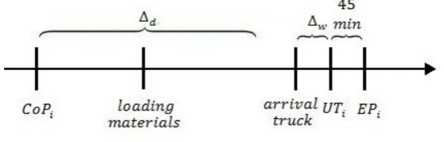
𝐶𝑜𝑃_𝑖. After a Call off Point the corresponding supplier processes the order. This means that the required materials are picked such that those materials are ready to be loaded into the truck. At the moment that a truck of the transporting company, HSL, arrives at the supplier, the materials are loaded into the truck. That truck delivers the materials directly to the Deventer plant. Depending on if there is another truck that uses the dock at that moment or not, the oncoming truck either has to wait until the dock become free or can directly start to unload the materials. The possible waiting time of the truck at the Deventer plant is denoted by ∆_𝑤. The goal is to reduce this waiting time to zero by scheduling the trucks in a smart way. If the dock is free, the truck starts unloading the delivery of order 𝑖. This time is denoted by

𝑈𝑇𝑖. After the unloading of the truck the materials are distributed to the designated areas in production. This is done by the same workers that unloaded the truck. The unloading of a truck and the distribution to the production areas takes about 45 minutes. This means also that during that time no other trucks can unload their materials. The moment that all the materials of order 𝑖 are distributed among the production area is denoted by 𝐸𝑃_𝑖. The times 𝑈𝑇_𝑖and 𝐸𝑃_𝑖

are related by the following equation:

(13)

13

The time that it takes to deliver the materials to the Deventer plant is called the delivery time. It is defined as the time from the Call off Point until the time that the truck begins unloading the materials. The minimum delivery time is the least amount of time that it takes to deliver the materials to the Deventer plant and is denoted by ∆_𝑑. Due to a positive waiting time or due to a chosen strategy, the real delivery time can be longer than the minimum delivery time. Hence, the waiting time can be a part of delivery time. This leads to (2.2).

𝑈𝑇𝑖≥ 𝐶𝑜𝑃𝑖+ ∆𝑑 _(2.2)

An overview of the delivery process is given in Figure 2.1. It shows a time line where the delivery process from the Call off Point to the moment the truck is finished unloading the materials are displayed. There is a difference between the arrival of the truck at the Deventer plant and the moment the truck starts unloading, namely the waiting time ∆𝑤. Despite of this difference, in the following every time the arrival of the truck is mentioned, the waiting time is omitted, such that the arrival of the truck and 𝑈𝑇𝑖 are at the same time. In the next

[image:13.595.137.461.334.438.2]

subsection, the order process is explained in more detail and the restrictions concerning the order process are given.

Figure 2.1: Time line of the delivery process

2.2. Order process

In this subsection, a more detailed description is given of the order process. Furthermore, the restrictions concerning the order process are discussed. The order process is the process from the moment that the material is being used until the order is send to the supplier, the Call off Point. First, the process is explained for a single order. After that, the order process of consecutive orders for the same supplier is discussed.

At the Call off Point, the order is send to the corresponding supplier, but before that can be done, the order has to be filled. As mentioned in the previous section, Bosch uses an Enterprise Resource Planning (ERP) system to record the materials that are being used in production. This is done with help of the Kanban system, which is explained later in this section. The order is filled with all the materials from which the Kanban card is recorded in the ERP system before the Call off Point and which have not been processed by a previous order. Note that this is not the same as the amount of materials that are being used until the Call off Point due to the following reason: As discussed in the previous section, after a

(14)

14

Only then, the ERP system records that the material is being used. The maximum amount of time between the moment a material is being used and the moment the corresponding Kanban card is scanned, is denoted by ∆_𝑘.

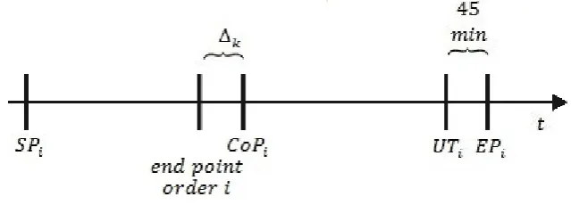
The above has the consequence that the materials that are being used after 𝐶𝑜𝑃_𝑖− ∆_𝑘 may go on the next order, because the corresponding Kanban cards may not be recorded into the ERP system before the Call off Point. In the following, we assume that the time 𝐶𝑜𝑃_𝑖− ∆_𝑘is the separation point between two consecutive orders, meaning that all material used until this time is assumed to be processed by order 𝑖. Hence, from this point in time, the materials used in production are assumed to be processed by order 𝑖 + 1. This point is time is called the start point of an order. At the same time, this is also the end point of the previous order. The start point of order 𝑖 is denoted by 𝑆𝑃𝑖. Shifting the above to get the equation for 𝑆𝑃𝑖 leads to the following:

𝑆𝑃𝑖 = 𝐶𝑜𝑃𝑖−1− ∆𝑘 _(2.3)

An overview of the order process is given in Figure 2.2. It shows a time line where the order process of order 𝑖 from the start point of the order to the moment the truck is finished

[image:14.595.137.457.364.479.2]

unloading the materials are displayed. Note that the end point of order 𝑖 is equal to the start point of order 𝑖 + 1.

Figure 2.2: Time line of the order process

Multiple orders

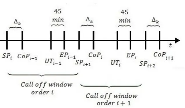
In the above, the order process of a single order was described. In the following, several consecutive orders for the same supplier are considered.

(15)

[image:15.595.157.475.78.264.2]

15

Figure 2.3: Time line of the order process of multiple orders

2.3. Scheduling trucks

In the previous subsections the order and delivery processes were described. To ensure that the trucks do not arrive at the same time, their arrival times must be regulated. In this subsection the process of scheduling the trucks at the Deventer plant is discussed.

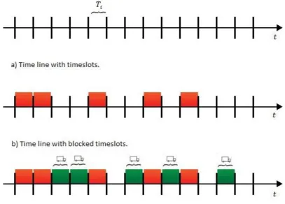
At the moment the truck arrives at the Deventer plant to deliver the materials, the truck could start to unload. This takes 45 minutes and within this time no other truck can unload materia ls at the Deventer plant. This is because there is only one dock present at the Deventer plant for unloading these materials and the truck that is being unloaded uses this dock completely. Hence, the dock is occupied for 45 minutes after a truck starts to unload materials. Based on the above, within the Integrated Supply Model timeslots of 45 minutes can be used. The reduction to a limited and quite small number of timeslots reduces the number of solutions to the scheduling problem for the unloading of the trucks. In the following the 𝑖-th timeslot is expressed as 𝑇𝑖.

Within the ISM, only the trucks of HSL are being scheduled. However, not all possible timeslots may be available for the trucks. This can be due to the opening hours of the suppliers, the lunch break of the workers in the department of internal logistics or due to an arrival of a truck of Veenstra. This results in a list of timeslots that are blocked and only the remaining timeslots are available for the trucks of HSL to deliver the materials. Possible approaches to schedule the trucks of HSL described in the Section 3. An important restriction is that the trucks of one supplier must arrive in the same sequence as the orders are sent to the suppliers. This means that the truck corresponding to order 𝑖 arrives earlier than the truck corresponding to order 𝑖 + 1. This leads to (2.4).

𝑈𝑇_𝑖 < 𝑈𝑇_𝑖+1

(2.4)

The timeslots are illustrated in Figure 2.4. In part a), the timeslots are shown without

(16)

16

[image:16.595.80.488.173.465.2]

As mentioned earlier, the trucks are scheduled following one of the approaches described in the next section. However, for this schedule, it remains to specify how the Call off Points are determined as they determine the amount of materials that is on the corresponding order. Hereby is important that the total amount of materials has to fit into one truck. In the next subsection more details on this process is given.

Figure 2.4: Time line with timeslots

2.4. Kanban process

In the previous subsections the timing of an order has been described. It remains to specify which quantities are assigned to an order. Hereby it is important that the amount of materials on an order must be such that it does not exceed the capacity of the truck. Furthermore, the production must not come to a standstill. In this subsection, first the method to measure the space that materials take up in a truck is explained. After that, the capacity restriction is formulated. Then, the method to ensure that the production does not come to a standstill is discussed and the accompanying restrictions are formulated. An important factor to ensure this is the number of Kanban cards available in the system. At the end of this subsection, first the replenishment time is explained and afterwards the other factors that are needed to

(17)

17

The start points of the Call off windows must be chosen such that the total amount of materials in the corresponding Call off windows fit into one truck. The space in a truck is expressed in floor places, which is the space one pallet takes up. To measure if the total amount of materials does not exceed the capacity of the truck, the floor place index is used.

The floor place index states how many floor places one piece of a material takes up in a truck. Hereby it has to be taken into account that, for some materials, the pallets can be stacked on top of each other, depending if the material is rigid enough. For example if 4 pieces of material 𝑗 go on one pallet and 2 pallets can be stacked on top of each other, one piece of material 𝑗 has a floor place index of 1/8.

The number of floor places an amount 𝛼_𝑗 of material 𝑗 with floor place index 𝑓𝑝𝑗 takes up, is denoted by 𝑓𝑝_𝑗(𝛼_𝑗) and can be calculated by 𝑓𝑝_𝑗(𝛼_𝑗) = 𝛼_𝑗∗ 𝑓𝑝_𝑗. This is not rounded up, because the different materials can be stacked on top of each other. The capacity of a truck,

𝐶𝐴𝑃, is also expressed in number of floor places. For each order, the total number of floor places that all the materials on that order take up, must be less than the capacity of the truck. If 𝛼_𝑗𝑖, … , 𝛼_𝑚𝑖 _{denotes the ordered quantities on order}_𝑖_{, this leads to the following constraint:}

∑ 𝑓𝑝𝑗( 𝑚

𝑗=1

𝛼_𝑗𝑖) ≤ 𝐶𝐴𝑃

(2.5)

Constraint (2.5) discusses the capacity restriction of the quantities that are assigned to an order. The other restriction is that the production must not come to a standstill. To ensure this, it is important to know the quantities of materials that are used in production. With these quantities, the amount of materials that must be ordered such that the same inventory level is maintained, can be determined.

Denote by 𝑞_𝑗(𝑡) the quantity of materials used in production at moment 𝑡 and let the amount of material 𝑗 that is used in production between two moments in time 𝑡1 and 𝑡2be denoted by

𝑄𝑗([𝑡1, 𝑡2]). Then the following is true:

𝑄_𝑗([𝑡₁, 𝑡₂]) = ∫ 𝑞_𝑗(𝑡)𝑑𝑡

𝑡2

𝑡1 (2.6)

Let the inventory level of material 𝑗 at moment 𝑡 be denoted by 𝐼𝑗(𝑡). The materials that are on order 𝑖 are delivered to the Deventer plant at 𝑈𝑇𝑖. 45 Minutes later all the materials are delivered to the corresponding section at the production area. At that moment, denoted by

𝐸𝑃_𝑖, the inventory levels are restocked. The next moment that the inventory levels get restocked is at 𝐸𝑃_𝑖+1. In between those moments the inventory levels only decreases due to the quantity of materials that are used in production. Because the production comes to a standstill if the inventory level of any material becomes zero, the following constraint ensures that this does not happen:

(18)

18

To record the quantities of materials that are being used in production, Bosch uses the Kanban system as discussed in Section 1.3. The Kanban system works with Kanban cards that record the materials that are being used and must be ordered again. The quantities 𝛼_𝑗𝑖 of material 𝑗 on order 𝑖 are the materials that are being used between 𝑆𝑃_𝑖 and 𝑆𝑃_{𝑖 +1}. This is expressed in (2.7):

𝛼_𝑗𝑖 = 𝑄𝑗([𝑆𝑃𝑖 , 𝑆𝑃𝑖+1]) _(2.8)

Note that 𝑆𝑃𝑖+1 is not a moment in the future since it lies before 𝐶𝑜𝑃𝑖 , the Call off Point of order 𝑖 , as shown in Figure 2.3. This means that the Kanban system is based on quantities of materials that are used in the past instead of in the future. A consequence of this is that first, a material has to be used before it is ordered, while the expression of (2.7) is based on ordering the materials that are needed in the future.

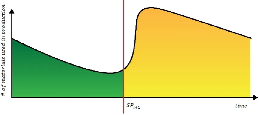
The above leads to a problem, which can be explained using Figure 2.5. In this figure the quantity of materials used in production during some time period are given and the red line indicates the end point of order 𝑖. Note that this is the same as the start point of order 𝑖 + 1. As the amount of materials used in production changes strongly at this Call off Point, a problem may occur. All the materials used during the green period are reordered within order

𝑖, but the production needs all the materials used within the yellow period to produce all the required heating boilers. Obviously, this may lead to a standstill if the inventory levels are not high enough to cope with this increased quantity of materials.

[image:18.595.82.514.391.582.2]

Figure 2.5: The problem of the Kanban system

(19)

19 Replenishment time

Although the Kanban system is based on the materials used in the past, a proper choice of the number of Kanban cards per material can ensure that the inventory levels remain high enough to prevent a standstill in production. For determining this number of Kanban cards, the

replenishment time is important. It measures the time that it takes to order and deliver the materials. The replenishment time is recorded from the moment a material is used in production until the material is delivered to the same section in production.

Measuring the replenishment time exactly for each material individually is often difficult and therefore the maximum replenishment time is taken for each order. This maximum

replenishment time of order 𝑖, denoted by 𝑅𝑇_𝑖, is given as the time between 𝑆𝑃_𝑖 and 𝐸𝑃_𝑖. Hence, it measures the first possible time that a material, that is on order 𝑖, is used in

production and it ends with the time that all the materials are delivered to the corresponding section in production. This leads to:

𝑅𝑇_𝑖 = 𝐸𝑃_𝑖− 𝑆𝑃_𝑖

(2.9)

[image:19.595.137.457.425.637.2]

In Figure 2.6, the replenishment time is shown. This figure shows the same time line as in Figure 2.3. Note that during the replenishment time, both the truck of order 𝑖 as well as the truck of order 𝑖 − 1 arrives to deliver materials.

Figure 2.6: Replenishment time

Number of Kanban cards

(20)

20

The determination of the number of Kanban cards is discussed in this subsection. However, first the importance of the Kanban cards is explained.

The Kanban card is an important factor in the Kanban system. Without these cards, no materials are ordered. Every time all the materials on a pallet are used, the corresponding Kanban card is send to the department of internal logistics to order those materials. The number of Kanban cards per material is essential to prevent that the production comes to a standstill. When there is only one Kanban card, there will be a standstill when all the

materials on the pallet corresponding to that Kanban card are being used. Hence, there should always be another Kanban card for the same material in the inventory, such that the materials on the pallet corresponding to the second Kanban card can be used in production. However, if there are too many Kanban cards of a material in circulation, the inventory level of that material becomes too high. As a consequence, the holding costs are higher and more space is needed to store all the materials.

Depending on four factors that influence how much Kanban cards are needed per material, the number of Kanban cards differs. These factors are the demand per day, the minimum order quantity, the replenishment time and the number of working hours per day. The first factor is the demand per day 𝑑 of material 𝑗, denoted by 𝐷_𝑗𝑑. In the Integrated Supply Model, this is equal to the quantity of materials that is used in production during day 𝑑. If the demand is high, there are more Kanban cards needed than if the demand is low, because the materials deplete more quickly and thus, a higher inventory level is needed. The maximum is taken over all the days of the week. The maximum demand of material 𝑗 per day, denoted by 𝐷_𝑗, is:

𝐷_𝑗 = max

𝑑 𝐷𝑗

𝑑

(2.10)

The next factor is the minimum order quantity of material 𝑗, denoted by 𝑀𝑂𝑄_𝑗. This is the amount per Kanban card. If the minimum order quantity (MOQ) is low, there are more Kanban cards needed than if the MOQ is high, because a low number of materials can be ordered, the inventory runs out more quickly. The third factor is the replenishment time, as discussed earlier. If the replenishment time is high, there are more Kanban cards needed than if the replenishment time is low. The last factor is the working hours per day of material 𝑗, denoted by 𝑊_𝑗. This is the number of hours per day that material 𝑗 can be used for production. This depends on the production line(s) at which the material is used. The working hours are used to scale the replenishment time such that only relevant hours are measured.

The number of Kanban cards of material 𝑗 needed for order 𝑖, denoted by 𝐾_𝑗𝑖, is based on the quantity of materials that are used in production during the replenishment time, that is from

𝑆𝑃𝑖 until 𝐸𝑃𝑖. The actual number of Kanban cards is achieved from this quantity by dividing it by the number of materials per Kanban card, 𝑀𝑂𝑄𝑗:

𝐾_𝑗𝑖 = ∫ 𝑞𝑗(𝑡)𝑑𝑡 𝐸𝑃𝑖

𝑆𝑃𝑖

(21)

21

Remember from (2.6) that the integral from (2.11) is equal to 𝑄_𝑗([𝑆𝑃_𝑖 , 𝐸𝑃_𝑖]). The actual number of Kanban cards of material 𝑗 needed to prevent running out of material 𝑗, denoted by

𝐾_𝑗, is the maximum number of Kanban cards over all orders:

𝐾_𝑗 = max

𝑖 𝐾𝑗

𝑖

(2.12)

The problem with these calculations is that 𝑆𝑃_𝑖, 𝐸𝑃_𝑖 and 𝑞_𝑗(𝑡) vary on a daily basis. To overcome this, an approximation is used. An upper bound is chosen for the determination of the number of Kanban cards. This upper bound is also used by Bosch and is described by Y. Sugimori et al. in [SKCU77].

For the upper bound of (2.12), the replenishment time, 𝑅_𝑗, is taken as the maximum replenishment time of all orders of the next week consisting of material 𝑗:

𝑅_𝑗 = max

{𝑖|𝑗∈𝑖}𝑅𝑇𝑖 _(2.13)

The number of Kanban cards of material 𝑗, denoted by 𝐾_𝑗, is now calculated in the following way:

𝐾_𝑗 = 𝐷𝑗 𝑀𝑂𝑄𝑗

∗ 𝑅𝑗

𝑊_𝑗 + 1 (2.14)

The four factors in (2.14) are consistent with observations made above about the number of Kanban cards. Furthermore, the term 𝐷𝑗

𝑀𝑂𝑄𝑗 is number of Kanban cards of material 𝑗 per day.

The term 𝑅𝑗

𝑊_𝑗 is the number of replenishments per day. The resulting number of Kanban cards,

𝐾_𝑗, is corrected with a safety factor which ensures that there are enough Kanban cards such that the production certainly does not come to a standstill.

2.5. Overview

(22)

22

In the Integrated Supply Model three decision variables are present: The Call off Point, the moment of the truck arrival and the number of Kanban cards. The Call off Point must be chosen such that the order does not exceed the capacity of the truck. The moment of the truck arrival must be chosen such that the truck delivers materials at a time when the workers at the Deventer plant can unload the truck. If the number of Kanban cards is fixed, an upper bound of the replenishment time can be determined.

If two of these decision variables are known, the third can be calculated. If the Call off Point and the moment of the truck arrival are known, the replenishment time can be calculated. With the replenishment time, the number of Kanban cards can be determined.

If the number of Kanban cards is known, the maximum replenishment time can be calculated. If the Call off Points are also determined, the upper bound on the arrival times can be

calculated by adding the maximum replenishment time to the Call off Points. This moment is an upper bound of the time that every material is delivered to the section at the production area. Thus, if for order 𝑖, 𝐶𝑜𝑃𝑖 is known, an upper bound of 𝐸𝑃𝑖 can be determined and from (2.1) it is known that 𝑈𝑇_𝑖= 𝐸𝑃_𝑖− 45 𝑚𝑖𝑛. If the arrival times of the trucks are known instead of the Call off Points, the lower bound of the Call off Points can be determined by reversing the above calculations.

In the next section two approaches are explained, based on these decision variables. The first approach determines the times at which a truck should ideally deliver the material. This ideal moment is when the truck has a full load. If the truck cannot deliver the materials at that moment, another less ideal moment is determined. After fixing the arrival time, the Call off Point is fixed as ∆_𝑑 before the truck arrival time.

The second approach determines the next Call off Point as the last moment for which the capacity of the truck is not exceeded. If this ideal Call off Point is reached, the truck delivers the corresponding materials as soon as possible after the Call off Point, accounting for the moments when the truck cannot deliver materials to the Deventer plant.

With both approaches, the number of Kanban cards is determined such that the inventory level is high enough to prevent a standstill in production. This means that with these

(23)

23

3. Approaches

In the previous section, the Integrated Supply Model for solving the Bosch supply problem was explained. In this section two approaches for solving the supply problem are explained. The first approach focusses on the arrival of the trucks. The Call off Points are determined based on the truck arrivals, which are chosen as close to the ideal moment as possible. The second approach focusses on the Call off Points. Based on those chosen moments, the moment that the corresponding truck delivers the materials are determined. With both approaches the third decision variable, the number of Kanban cards, is determined based on the chosen Call off Points and truck arrivals. In this section, first the current approach for scheduling the trucks that deliver great volume materials is explained. Then, the assumptions for the ISM are discussed. After that, both approaches are explained. The limitations and potentials of both approaches are discussed next and finally one of the two approaches is extended to the Extended Integrated Supply Model (EISM).

3.1. Current Approach

Before explaining the two approaches developed to optimize the supply chain of Bosch, the current approach for ordering great volume materials is shortly discussed.

This approach predicts, for each day of the week, the number of trucks that are needed to deliver all the materials per supplier. The prediction is made on the basis of the production planning. The number of trucks is calculated with help of the floor place index. The day with the highest number of trucks is taken. This process is done for all suppliers such that for each supplier is known how many trucks are needed at most per day. These numbers of trucks are then used for every day of the week implying that there are always enough trucks to deliver the materials. This is done each week when a new production plan is made for the next week.

This approach obviously uses many trucks. To reduce the number of trucks, two new approaches are developed. Both approaches make use of the Integrated Supply Model described in the previous section. Before the two approaches are explained, the assumptions made are elaborated.

3.2. Assumptions

(24)

24

In Section 2.3, the scheduling of the trucks was discussed. In that section timeslots were mentioned and it was assumed that the Integrated Supply Model uses timeslots of 45 minutes. This coincides with the time that the dock is occupied by an unloading truck. The use of timeslots is not only necessary for scheduling the trucks, but also for the Call off Points and the time windows to measure the quantity of materials that are used in production. If we chose to use also timeslots of 45 minutes for these points, a limited and quite small number of timeslots is obtained. In a first step, the reduced solution space has to be chosen to be the solution space for the Integrated Supply Model. In the Extended ISM, the length of the timeslots is reduced to 15 minutes. This is done to have a better prediction of the quantity of materials that are used in production. As a consequence, the occupancy of the trucks will get higher.

The next assumption is about estimating the quantity of materials used in production. Due to agreements with HSL, the truck schedule for the whole week must be send to HSL at the end of the previous week. This truck schedule specifies a schedule of all trucks of HSL with the times when the trucks have to pick up the materials at the supplier and the times that the truck must deliver the materials at the Deventer plant. This schedule is fixed and cannot be changed during the week. As a consequence of this schedule, the Call off Points and the moments the trucks arrive must be determined a week in advance. Hence, the actual quantity of materials used in production cannot be used to determine the decision variables. Instead, a prediction has to be used to estimate the quantity of materials. This prediction is based on the production planning made a week in advance.

The production planning specifies for each day of the week the quantities of materials that are planned to be used for the production at that day. These values are calculated based on the number of production lines and the number of shifts in production. The Integrated Supply Model uses this information as input. It determines per timeslot the quantity of materials used in production by spreading the specified quantities evenly over the hours that the material is being used within the planned production scheme. Note that this number of hours can differ per material depending on the production line at which the material is used. Spreading the used materials evenly over the day is not completely accurate. The reason for this is that at some production lines multiple types of heating boilers are made. Within this mix it might occur that some types are produced more at the beginning of the day. As a consequence, the materials needed for the production of that type of heating boiler are used first, instead of that it is spread out evenly over the day.

The total quantity of materials used in production per timeslot is used to determine the Call off Points and the moments that the truck arrive at the Deventer plant. The method to determine this total quantity is shown in Figure 3.1.

As already mentioned, the prediction of the used amount of materials is not exactly the same as the actual use of materials. Next to the differences resulting from the mix at the production lines, also backlog or other unforeseen difference in production can lead to deviations.

(25)

25

The safety margin is denoted by 𝛾 ∈ [0,1] and specifies the fraction to which a truck may be filled in the planning. This means that the Call off Points are determined such that the truck should not be occupied more than 1 − 𝛾 times the capacity of the truck. When the truck is filled with the actual quantity of materials, the safety margin leaves space to cope with differences between the predicted and actual quantity of materials. In this way, all the materials still can be delivered in one truck to the Deventer plant.

This leads to the following constraint:

∑ 𝑓𝑝(

𝑚

𝑗=1

𝛼_𝑗𝑖) ≤ 𝐶𝐴𝑃 ∗ (1 − 𝛾)

(3.1)

In the next subsections, the two developed approaches are explained, but before that, the method to predict the quantity of materials used in production for each supplier is explained in more detail. The predicted quantity of material 𝑗 of supplier 𝑠 between timeslots 𝑡₁ and 𝑡₂ is denoted by 𝑃𝑄_𝑗𝑠([𝑡₁, 𝑡₂]). At each timeslot, the quantity of materials used from the first relevant timeslot until the current timeslot is calculated per material. This is used to determine the total quantity of material. The quantity of materials is expressed in number of floor places. The total number of floor places of the materials used in production of supplier 𝑠 until

timeslot 𝑡 is denoted by 𝑇𝐹𝑡𝑠. This process is shown in figure 3.1.

Figure 3.1: Method to determine quantity of materials used in production

3.3. Approach 1: Determine truck arrivals

In this subsection the first approach is explained. This approach focusses on the arrival of the trucks. The Call off Points are determined based on the moments that are chosen for the trucks to deliver the materials.

The moment a truck can start to unload the materials at the Deventer plant, 𝑈𝑇_𝑖, is derived using the Call off Point, 𝐶𝑜𝑃_𝑖, and the minimum delivery time to deliver the materials to the Deventer plant, ∆_𝑑. Remember from formula (2.2) that these times are restricted by 𝑈𝑇_𝑖 ≥ 𝐶𝑜𝑃_𝑖+ ∆_𝑑. This means that the truck corresponding to order 𝑖, that is send to supplier 𝑠, must arrive at least ∆_𝑑 time later than the time that order 𝑖 is placed. However, if the timeslot for

(26)

26

In Approach 1, the Call off Point is set exactly ∆𝑑 before 𝑈𝑇𝑖:

𝐶𝑜𝑃_𝑖 = 𝑈𝑇_𝑖 − ∆_𝑑 ∀𝑖

(3.2)

As the goal should be to have the trucks loaded as close as possible to their capacity, it still should be the goal to schedule the next Call of Point as close as possible to the preferred next Call of Point. This implies that the used arrival time of the truck, 𝑈𝑇𝑖, should be as close as possible to the truck arrival time which follows from the preferred Call of Point. Because of (3.2), this means that the Call off Point must be shifted backwards in time such that the truck arrives within a timeslot that is available.

It remains to specify how precisely the backward shifting is realized. Before that can be done, the approach is explained in more detail. For each timeslot, the method of Figure 3.1 is used to determine the total number of floor places used until the current timeslot. A matrix 𝑀 is constructed, where 𝑀𝑖,𝑗specifies when the truck should ideally arrive at the Deventer plant for each supplier 𝑖 when the last Call off Point was at timeslot 𝑗. This matrix is filled as follows: For position 𝑀_𝑖,𝑗, the total number of floor places of supplier 𝑖 at timeslot 𝑗 is used as starting point. Let 𝑝 be a counter starting at zero that goes up by one every time constraint (3.3) is not violated.

𝑇𝐹_𝑝+1𝑖 − 𝑇𝐹_𝑗𝑖 ≤ 𝐶𝐴𝑃 ∗ 𝛾

(3.3)

Eventually, this means that 𝑝 + 1 is the first number that would violate the restriction of (3.3). As a consequence, 𝑝 is the timeslot at which the truck would be as full as possible. The truck corresponding to the Call off window from timeslot 𝑗 to 𝑝 would arrive ∆_𝑑later, due to the assumption of this approach. Hence, the position 𝑀_𝑖,𝑗 is filled with 𝑝 + ∆_𝑑, the timeslot for which the truck from supplier 𝑖 arrives at the Deventer plant with a maximum load, if the previous Call off Point of supplier 𝑖 was at timeslot 𝑗. In Figure 3.2, an example of the matrix

𝑀 is shown.

Figure 3.2: An example of the matrix M(i,j)

Beginning at the start of the planning horizon, the moments that the trucks arrive at the Deventer plant are determined for each supplier. These moments come from the matrix 𝑀. The first timeslot is determined by checking position 𝑀_𝑖,1, the next Call off Point is ∆_𝑑 earlier than the timeslot shown at position 𝑀𝑖,1, 𝑘. For the next truck, position 𝑀𝑖,𝑘−∆𝑑 has to be

(27)

27

If all the trucks can be scheduled at these possible timeslots such that it results in a feasible schedule, this would lead to a schedule where the trucks are all as full as possible. But in this scheduling problem, it is possible that the assigned possible timeslots are already blocked due to lunch breaks, opening hours of the supplier or the arrival of a truck of Veenstra. If, due to a blocked timeslot or by an already scheduled truck, another truck could not arrive at the

assigned possible timeslot, it can only arrive earlier than the ideal timeslot. Otherwise, the corresponding Call off Point would be later, which means the capacity of the truck would be exceeded. The timeslot that is chosen for the arrival of that truck is the first timeslot that is closest to the ideal timeslot without violating constraint (3.1).

If a truck must arrive earlier, due to the fact that the ideal timeslot is blocked, the

corresponding Call off Point is not the only thing that changes. All the possible timeslots from the same supplier has to be determined again. Another problem that arises with the Integrated Supply Model becomes apparent when the transition has to be made between the weeks. If a truck has to arrive Monday morning, the order has to be sent the previous week. The ISM cannot cope with this. To overcome this problem, a restriction is introduced that ensures that the last truck of each supplier arrives at the Deventer plant Friday afternoon.

The scheduling problem that describes this problem is defined as follows: For each supplier 𝑖, let us define a vector of Call off Points 𝑐₁𝑖, … , 𝑐𝑛𝑖

𝑖 _with_𝑛

𝑗 the number of Call off Points of supplier 𝑖. For these 𝑐_𝑘𝑖 the following restriction must hold to ensure that the capacity restriction of the truck is not violated:

𝑚_𝑖,𝑐

𝑘𝑖 ≥ 𝑐𝑘+1

𝑖 _{+ ∆}

𝑑

(3.4)

Furthermore the last truck of all suppliers must arrive at the Deventer plant after a predetermined boundary, 𝐿:

𝑐𝑛𝑖

𝑖 _{≥ 𝐿}

(3.5)

All the Call off points 𝑐_𝑘𝑖 must be disjoint and must be unequal to a blocked timeslot. The aim is to find for all suppliers 𝑖 a sequence as specified above, where ∑ 𝑛_𝑖 is minimized. That is, minimize the total number of trucks.

This scheduling problem can be easily formulated as an Integer Linear Program (ILP), which is solved by the optimizing software called AIMMS. In the next section, the input and the implementation for this ILP is described.

3.4. Approach 2: Determining Call off Points

(28)

28

In the first approach, the delivery time was set to the minimum delivery time. By doing this, a problem arose if the truck could not deliver the materials at the preferred time. In that case, the timeslot of the truck arrival as well as the timeslot for the Call off Point was shifted backwards. This resulted in a smaller Call off window, what meant lower occupancy in the truck. The second approach solves this problem by fixing the Call off windows and shifting the timeslot that a truck can deliver the materials forwards instead of backwards.

For this approach a matrix 𝑁 is constructed. This matrix records when the Call off Points ideally has to take place for each supplier 𝑖 and timeslot 𝑗. These Call off Points are

determined in a similar way as for the matrix 𝑀. Let 𝑝 be a counter starting at zero that goes up by one every time constraint (3.3) is not violated. The next Call off Point for position 𝑁_𝑖,𝑗

is then 𝑁_𝑖,𝑝. Note that the only difference between matrices 𝑀 and 𝑁 is that matrix 𝑀 is filled with information about the moments when the truck arrives at the Deventer plant, while matrix 𝑁 is filled with information about when the next Call off Point takes place.

In detail, the second approach solves the Integrated Supply Model as follows: Beginning at the start of the planning horizon, determine the next Call off Point by checking 𝑁𝑖,1. Let the corresponding value be 𝑘. For determining the next Call off Point of the same supplier, 𝑁𝑖,𝑘 has to be checked and so on. This is done for all suppliers. In this approach, the Call off Points are now fixed and cannot be changed anymore. All that remains is to determine when the trucks can arrive at the Deventer plant. Note that in this approach not the complete matrix

𝑁 has to be calculated, but only the entrances of the calculated sequence of Call off Points. Ideally, the trucks all arrive exactly ∆_𝑑 later as the corresponding Call off Point. But, as with the first approach, it can occur that timeslots are blocked, due to reasons that are mentioned earlier. To solve this with the first approach, the truck had to arrive earlier such that the Call off Point had to be shifted backwards. As a consequence, the upcoming Call off Points had to be calculated again. By fixing the Call off Points and keeping the delivery times variable as in the second approach, if the ideal timeslot is blocked, the arrival of the truck can simply be shifted forwards until the first available timeslot is found. As a consequence, the Call off Points do not have to be calculated again. This leads to a sequence 𝑐₁𝑖, … , 𝑐𝑛𝑖

𝑖 _{of Call off Points} per supplier 𝑖, with 𝑛_𝑖 the number of Call off Points of supplier 𝑖. The next step is to

(29)

[image:29.595.200.382.69.437.2]

29

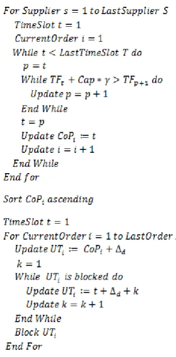
Figure 3.3: Approach two model

First, the Call off Points are determined. Afterwards, the Call off Points are sorted such that the first order is the one of which the Call off Point is first. Finally, the arrival times of the trucks are scheduled following the “Earliest release date first” technique. Note that this model accounts for the blocked timeslots and that if the arrival time of a truck is scheduled that timeslot also becomes blocked.

This approach also has a consequence. If the ideal timeslot for the arrival of the truck of order

𝑖 is blocked, the arrival time of that truck is shifted forwards in time. Because the

corresponding Call off Point is fixed, the time between the start point of the Call off window,

𝑆𝑃_𝑖 and the moment all materials are delivered to the corresponding section in production,

𝐸𝑃_𝑖, becomes longer. Remember from (2.9) that the replenishment time of order 𝑖 is 𝐸𝑃_𝑖 − 𝑆𝑃_𝑖. This means that the replenishment time becomes longer as a consequence of the second approach.

(30)

30

3.5. Discussion

In this subsection the potential and the limitations of both approaches are given. Based on this discussion, an adapted version of one of the approaches is presented in the next subsection.

The main difference between the two approaches is the length of the Call off windows. In the first approach, the Call off Points might get shifted backwards. As a result of which, the Call off windows are shortened, while with the second approach the Call off windows are always of maximum length. This means that the occupancy of the truck is higher using the second approach. Another benefit of Approach 2 is that the resulting scheduling problem is easier to solve than the scheduling problem of Approach 1, which had to be solved by optimization software.

The benefit of Approach 1 is that the maximum replenishment time is smaller or equal to the maximum replenishment time of the second approach. The reason for this is that with

Approach 1the arrival times of the trucks can only be shifted backwards, which has a positive effect on the replenishment time. With Approach 2, if a truck cannot be scheduled at the preferred timeslot, the arrival time is shifted forwards in time, which has a negative effect on the replenishment time. A longer replenishment time means more Kanban cards, which means higher holding costs and more space needed to store the materials.

A limitation of both these approaches is that they cannot cope with the transition between the weeks. For both approaches a restriction has to be formulated, which stated when the last truck of the week has to arrive per supplier. This results in trucks that arrive on Friday afternoon with low occupancy. When a transition can be made between two consecutive weeks, the truck could arrive early Monday morning, while the order was sent to the supplier Friday afternoon of the previous week. This would mean that the possible “extra” truck at the end of the week due to the restriction that states the arrival time of the last truck per supplier, can be removed. As a result, the scheduled trucks would have a higher occupancy and obviously fewer trucks are needed to deliver all the required materials to the Deventer plant.

Another limitation is that the approaches both use timeslots of 45 minutes. The length of the timeslots is not only used for the arrival times of the trucks, but also for the determination of the Call off Points and for the determination of the predicted quantity of materials used in production. These predictions would be more accurate if they were based on shorter time intervals. Above that, if the length of the timeslots would be smaller, also the Call off Points could be placed closer to the time at which the truck is as full as possible.

The last limitation is due to practical reasons. With the current approach, the trucks arrive at the same time every day. The corresponding order is also send to the supplier at regular times. This means that it is easy to remember when the orders has to be send, which means that barely any mistakes are made by the workers of Bosch as well as by the workers of the

(31)

31

After some discussion within Bosch, it has been chosen to modify Approach 2. This approach is modified to overcome some of the above mentioned disadvantages. The main reason to choose for Approach 2 is that it makes optimal use of the capacity of the trucks. Another reason is that the resulting approach has to be also implemented in the real world, as the scheduling problem, corresponding to Approach 2, is easier to solve than the scheduling problem corresponding to Approach 1. These advantages have outweighed the disadvantage of the longer replenishment times.

3.6. Extended Integrated Supply Model

In this subsection, the Extended Integrated Supply Model is presented. The EISM is an adapted version of the Approach 2 model described in Section 3.4. The changes made to the Approach 2 model are explained in the following.

One of the limitations of the Approach 2 model is that it could not cope well with the

transition between consecutive weeks. This is solved by not only determining the arrival times of the trucks for the five days of the current week, but also for the first day of the next week. In this way, if a truck has a Call off Point that takes place at Friday afternoon, it may be planned to arrive at the Deventer plant the “next” morning, just as any other truck. All the arrival times of the trucks that arrive the next week are recorded and regarded as fixed input for the truck schedule of the next week.

The limitations that the length of timeslots must be 45 minutes and that the variations of the unloading patterns per supplier are irregular, are solved within one adaption in the following way. For each supplier, the maximum number of trucks per day during the whole year is estimated. This estimation of the maximum number of trucks for supplier 𝑠 is denoted by

𝑁𝑜𝑇𝑠. For each supplier 𝑠, 𝑁𝑜𝑇𝑠 timeslots are reserved for a possible arrival of a truck of supplier 𝑠. These reserved timeslots for supplier 𝑠 are denoted by the set 𝑃𝑇𝑠. The trucks can only arrive at one of the reserved timeslots of its supplier. Note that not all the reserved timeslots have to be used for the arrival of a truck. The reserved timeslots have to be chosen such that the time between two consecutive reserved timeslots of any supplier is at least 45 minutes. This is the time that is needed to unload the truck.

The choice of the reserved timeslots is based on tests with different compositions of timeslots. The aim is to choose the reserved timeslots in a way such that the maximum replenishment time is minimized. The test with a composition that all reserved timeslots are bundled together, had the longest maximum replenishment time. With this composition, the average time between the preferred truck arrival time and the first available reserved timeslot was the longest. Eventually, a composition is chosen where the reserved timeslots are spread out over the day, while still accounting for the opening hours of the suppliers. Note that all the

reserved timeslots of the suppliers are disjoint.

It remains to specify how it is determined which reserved timeslots a supplier uses for its truck arrival and which not. To determine this, the scheduling of the trucks is slightly adapted compared with the Approach 2 model. First, the Call off Points of supplier 𝑠 are determined as with the Approach 2 model and the truck is scheduled to arrive at least ∆_𝑑 later than the corresponding Call off Point. From that point in time, the first available timeslot from the set

(32)

32

In the adapted model, the length of the timeslots on the production side has been chosen to be 15 minutes, which is the acceptable interval to determine the predicted quantity of materials. This reduced length on average leads to a higher occupancy of the trucks, as it may take 15 or 30 minutes longer until the capacity constraint (3.1) is violated.

The limitation that with the ISM the trucks arrive at irregular times is overcome by introducing the reserved timeslots. With the introduction of the reserved timeslots, the

timeslots are dedicated to only one supplier, which decreases the chances of making a mistake with sending the orders and unloading the trucks.