Parallel combinator reduction : some performance bounds

http://wrap.warwick.ac.uk/

Joy, Mike and Axford, T. H. (1992) Parallel combinator reduction : some performance bounds. University of Warwick. Department of Computer Science. (Department of Computer Science Research Report). (Unpublished) CS-RR-210

Permanent WRAP url:

http://wrap.warwick.ac.uk/60899

Copyright and reuse:

The Warwick Research Archive Portal (WRAP) makes this work by researchers of the University of Warwick available open access under the following conditions. Copyright © and all moral rights to the version of the paper presented here belong to the individual author(s) and/or other copyright owners. To the extent reasonable and practicable the material made available in WRAP has been checked for eligibility before being made available.

Copies of full items can be used for personal research or study, educational, or not-for-profit purposes without prior permission or charge. Provided that the authors, title and full bibliographic details are credited, a hyperlink and/or URL is given for the original metadata page and the content is not changed in any way.

A note on versions:

The version presented in WRAP is the published version or, version of record, and may be cited as it appears here.For more information, please contact the WRAP Team at:

Mike Joy

Department of Computer Science, University of Warwick,

COVENTRY, CV4 7AL,

UK

e-mail: [email protected]

Tom Axford

School of Computer Science, University of Birmingham,

PO Box 363, BIRMINGHAM,

B15 2TT, UK

e-mail [email protected]

Copyright © 1992 M.S. Joy and T.H. Axford. All rights reserved.

ABSTRACT

A parallel graph reduction machine simulator is described. This performs combi-nator reduction and can simulate various different parallel reduction strategies. A number of functional programs are examined, and experimental results presented comparing the amount of parallelism obtainable using explicit divide-and-conquer with the maximum amount of parallelism available in the programs.

1. Introduction

In recent years functional languages [8] have gained popularity, since translating a formal specification of a problem to an executable functional program is (relatively) straightforward. Imperative language constructs model closely the hardware structures of conventional (von Neumann) architectures. Functional languages, however, were not designed with any architecture in mind, and as a result, implementations of functional languages on present-day machines tend to be relatively slow. The question of how to speed up functional language implementations is therefore one which must be addressed in order for their benefits fully to be realised.

One way of running a program faster is to execute it on several processors simultaneously. Functional lan-guages contain no notion of "state", and many synchronization problems present with parallel imperative programs are absent from parallel declarative programs. Thus simultaneous execution of sections of a func-tional program on different processors should present relatively few problems.

There are several different approaches [16] to the problems of parallelising the evaluation of a functional program. Most of these fall into one of two categories. Firstly, the high-level program may be annotated explicitly to instruct how the parallelism should be achieved. Secondly, the source program can be anal-ysed automatically using techniques such as strictness analysis in order to determine which sections of the program may be executed concurrently. We hav e written a simulator for a shared-memory multiprocessor which can model various strategies for parallelising a functional program using combinator graph reduc-tion.

Our interest is in the implementation of functional languages using combinator graph reduction, and in par-ticular in the extent to which parallel evaluation can be exploited. To this end we have been investigating the generic properties of a fixed translation scheme. The transformation from a functional program to a combinator graph is a complex procedure which can be accomplished using various algorithms, and it was therefore important to deal with a default translation strategy.

We introduce the concept of saturation parallelism. Giv en a translation of a functional program to a com-binator graph, there are sections of the graph which can be evaluated simultaneously; if a parallel machine evaluates all such sections in parallel, then we describe that evaluation strategy as saturation parallelism. For an idealized machine with unlimited processors and zero communication costs, this strategy will pro-vide a measure of the minimum time necessary to evaluate that program, and thus propro-vide a base-line against which the performance of other parallel evaluation strategies can be measured.

This paper reports the results of experiments with different strategies for parallel evaluation. We hav e run some benchmark programs using (a) explicitly introduced parallelism and (b) saturation parallelism. The examples we have chosen are such that explicit parallelism can be introduced in a natural fashion.

2. Combinator Graph Reduction

The particular implementation method for functional languages which interests us is combinator graph reduction. We can think of a combinator as a simple function. Using combinators to evaluate a functional program involves first of all taking that program, thought of as a sugared lambda-expression, and "abstract-ing" the variables. All lambda expressions are thus removed and combinators introduced. So a program containing names and value-bindings is translated to an equivalent expression containing no names, and the resulting expression contains only combinators, together with basic data. An implementation which did not abstract names would need to keep track of the partially-evaluated expressions associated with each name, a significant communication overhead.

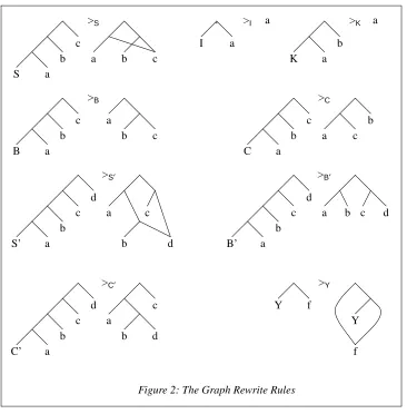
This expression can then be considered as a graph, where the application of a function to an argument is represented as a binary node, and an atomic datum or a basic combinator is a leaf node. The graph may not necessarily be a tree, as sharing of common subgraphs may take place, and in the case of recursive func-tions, that sharing may cause cycles to be introduced into the graph.

2.1. Sets of Combinators

Some preliminary observations on our choice of combinators are appropriate at this point. We work with combinators as presented originally by Curry [3] , although this formalism is not the only way of describing combinatory logic (categorical combinators, for instance, create a powerful theory which has also been used as a basis for graph reduction machines). For the purposes of this paper we identify two principal classes of combinators. Firstly, combinators which form a (small) fixed set, such as Turner’s combinators [20,21] , and secondly combinators which form an extensible set and which may be created when required, such as Supercombinators [11] .

The former class has the advantage of being simple to use and to reason about, but yields combinator expressions which are relatively large and complex [10] . The latter class requires sophisticated abstraction techniques, and typically combinators will represent compiled functions which can be run on conventional architectures fairly efficiently. In [5] Hartel presents statistics indicating that, using various metrics, the speed of evaluation (measured by combinator reduction steps) of this latter class of combinators compared with a fixed set is better by typically less than an order of magnitude.

A benefit of having a fixed combinator set is that an architecture can (in theory, at least) be devised so that the combinators are implemented in hardware. Novel coding techniques [13,15] can also be employed to reduce the space wastage inherent in a naïve implementation of such a fixed combinator set. Most current work relating to parallel combinator reduction however assumes an extensible combinator set.

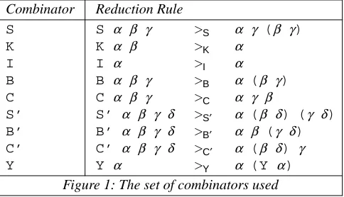
We hav e examined combinator reduction involving various fixed combinator sets. In this paper we consider one particular choice of combinators, the set originally introduced by Turner [20,21] . They are defined in Figure 1 (α,β,γ,δrepresent arbitrary expressions), where the reduction rule for each combinator is given.

Combinator Reduction Rule

S S α β γ >S α γ (β γ)

K K α β >K α

I I α >I α

B B α β γ >B α (β γ)

C C α β γ >C α γ β

S’ S’ α β γ δ >S′ α (β δ) (γ δ)

B’ B’ α β γ δ >B′ α β (γ δ)

C’ C’ α β γ δ >C′ α (β δ) γ

Y Y α >Y α (Y α)

Figure 1: The set of combinators used

. >I a

I a

>K a

K a b >S S a b c

a b c

>B B a b c a b c >C C a b c a b c

>S′

S’ a b c d a b c d

>B′

B’ a

b c

d

a b c d

>C′

C’ a b c d a b c d >Y Y Y f f

Figure 2: The Graph Rewrite Rules

2.2. Parallelism

A number of projects have recently examined parallel graph reduction for functional languages. Some of these use an extensible set of combinators, such as GRIP, MaRS, Alfalfa and the Evaluation Transformer model. Several are not based on combinators, such as Alice, Flagship, the <ν,G> Machine, the ABC-Machine and Rediflow.

Given a large combinator graph, it is likely that many nodes in the graph can be rewritten concurrently. Due to the small granularity of the combinators, combinator graph reduction is a candidate for massive par-allelism [6] . New generations of computers, such as custom-made VLSI architectures and Neural Machines place us within sight of an efficient parallel graph reduction machine.

Unfortunately, it is not always easy (or necessarily even possible) to decide which graph nodes need to be rewritten, and which do not (such as the unused arm of a conditional). The technique of lazy evaluation on a single processor will minimise the amount of work necessary to reduce a graph, but does not lend itself to identifying opportunities for parallelism on a multiprocessor.

Various strategies for parallel graph reduction have been examined, such as load balancing amongst the available processors [19] and strictness analysis [7] . Given a specific fixed combinator set, we examined the time efficiency of executing a program using two different strategies:

(i) saturation parallelism (rewriting sections of graph in parallel whenever it is possible to do so), and

Saturation parallelism is in general not a practical technique because it involves an unbounded number of processors. It is, however, useful since it gives us an indication as to the maximum amount of parallelism available in a program, against which we can measure how close to optimal speedup "real" strategies come. Explicit parallelism, on the other hand, is a powerful technique if used correctly. Its main disadvantage is that the onus is placed upon the programmer to code a program and identify the parallelism in it correctly. We hav e a upper bound on the speed of a parallel evaluation of a combinator graph, namely that with satu-ration parallelism. We hav e also introduced explicit parallelism by using a simple divide-and-conquer approach (see section 6 below). Other more sophisticated attempts at achieving parallelism would be expected to yield a performance between the upper bound of saturation parallelism and that given by our explicit parallelism.

3. The Graph Reduction Machine

The simulator takes as input GCODE [12] , which is a textual description of a graph representing a func-tional program. GCODE contains lambdas, combinators, basic operators (delta combinators), integers, real numbers, and sum-product domains. The GCODE is generated from FLIC [17] which is minimally sug-ared lambda-calculus. The input is then compiled to abstract variables and introduce combinators [20,21] . Recursion is handled by the "Y" combinator. The resulting graph is acyclic, and the reduction rule for the "Y" combinator preserves this property.

Reduction of the graph takes place by rewriting several parts of it concurrently. The usual serial lazy evalu-ation strategy is embedded within this parallel reduction strategy, in the sense that at any stage in the reduc-tion process the next reducreduc-tion step in the lazy evaluareduc-tion strategy will always be one of the several concur-rent reduction steps in our parallel strategies.

3.1. Architecture

The simulated machine has a fixed number of processors, on which may run a variable number of pro-cesses. Each process rewrites a section of graph until one of the following conditions is reached:

• that section becomes a datum (integer, floating point number, or sum-product);

• that section cannot evaluate further (when an operator is presented with too few arguments);

• that process is destroyed by another process.

A specific process will not recursively evaluate elements of a sum-product domain, but will spawn further processes if required. A process contains (inter alia) two stacks, a status value and a priority value.

Each processor is either allocated a single process and is Busy, or is awaiting a process and is Fr ee. A pro-cess may have status Running if in the propro-cess of rewriting a section of graph, Suspended if awaiting the result of another process before evaluation may proceed, or Waiting if it is able to continue running but has not been allocated to a processor.

A process is allocated a "priority", which is either Possible or Needed. A Needed process is one which is known to be required to be evaluated by the lazy evaluation strategy. A Possible process is one which may require evaluation.

Three queues of processes are maintained; one contains the Running processes, one the Waiting processes, and one the Suspended processes. The elements of each queue are ordered by process priority.

A "master process" controls the allocation of processes to processors, and will perform the administration of the processes and their allocation to processors, as follows:

• Each queue has its elements ordered by Priority, with Needed processes at the head of the queue.

• When a process in the Running queue completes execution, that process ceases to exist and the pro-cessor allocated to it becomes Fr ee.

• If a process becomes Suspended, it is placed in the Suspended queue and the processor allocated to it becomes Fr ee.

• A processor which is Fr ee is allocated to the process at the head of the Waiting queue. If the Waiting queue is empty that processor simply remains Fr ee.

• If all processors are Busy, and one of the Running processes has priority Possible, and one of the Waiting processes has priority Needed (which we may assume to be at the head of the Waiting queue), then that Possible process is swapped with the head of the Waiting queue.

The machine runs in time measured by "cycles". In one cycle a process will perform one reduction step, and the master process will handle any tasks which this may generate. At the start of each cycle the master process ensures that each processor which can be allocated a process is allocated one, and that each Run-ning process is known to be able to perform a reduction step. Each processor then causes the process allo-cated to it to perform one single combinator reduction.

At the start of a program execution, after the combinator graph has been created, a single process is created with priority Needed, which will begin to rewrite the graph using the standard lazy algorithm. Where nec-essary it will create other processes with priority Needed, or indicate to the master process that other pro-cesses with priority Possible should have priority updated to Needed. Further propro-cesses may be created as dictated by the parallel evaluation strategy.

3.2. Lazy Evaluation

It will be clear from the above description that the number of Needed graph reduction steps will be pre-cisely the number of steps necessary to evaluate a program using lazy evaluation on a single processor. Thus the number of cycles taken for the multiprocessor simulator to evaluate a program will be no more than the number of steps to evaluate a program using lazy evaluation. Our system of Queues guards against the danger of speculatively offshipped processes being evaluated instead of required processes and thereby causing performance degradation.

3.3. Shared Memory

For the purposes of this exercise we have deliberately left out of our calculations overheads associated with communication between processors. Since we wished to examine the effect of the idealised situation where unrestricted parallelism was available the effect of introducing extra metrics into the calculations would have been a distraction. The assumption of a shared-memory multiprocessor was felt to be the simplest way to simulate such an idealised machine. Indeed, the machine resources we had available to use were only just sufficient to perform the experiments reported here, and simulation of a distributed processor would undoubtedly have been infeasible.

3.4. Overheads

Much of the workload relating to moving processes between processors is left in the control of the master process. In a worst-case example, this process could do constant amount of work for each processor each cycle. By implementing the master process so that its functions are distributed about the processors, this work would then involve constant extra time per cycle. The process has been implemented in the way described for reasons of improving the clarity of the software.

4. The Parallel Evaluation Strategies

We consider two parallel evaluation strategies. These are described in terms of the creation of new pro-cesses and their allocation to specific processors; subsequent management of propro-cesses is as described above.

4.1. Strategy 1: Saturation Parallelism

For instance, consider the following combinator expression (α,β,γ,δandεrepresent arbitrary expressions):

B (B α β) (C γ δ) ε

After one reduction step, fired by the leftmostB, we get

B α β (C γ δ ε)

In this expression both theBandCcombinators have sufficient arguments. TheB-reduction will be per-formed by the same process as the previous reduction (and on the same processor), and a new process (with priority Possible) will be created to handle theC-reduction. This latter process will then be placed in the Waiting queue, and consequently reduced by another processor when one becomes Fr ee. If the parent pro-cess in due course attempts to perform the reduction it has offshipped, the parent propro-cess will be Suspended until the child has performed that reduction.

This results in a large set of processes, most of which will have priority Possible, and many of which will be short-lived. The overheads of managing large numbers of processes are high, since many of them will return results which are not required; this strategy is intended as a benchmark against which we can mea-sure the extent to which other strategies exploit available parallelism. We obtain a figure which is the mini-mum time (measured in cycles) for the graph to evaluate fully.

4.2. Strategy 2: Explicit Parallelism

Initially, only one process is created, as described in the previous section. Subsequently processes are flagged so that they will be queued to run on their parent processor only. Conceptually, each processor has its own private triple of Running, Waiting and Suspended queues.

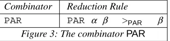
Whenever a section of code has to be sent to a different processor (when the combinator PAR [18] is encountered) a process is created and offshipped to another processor with empty Running and Waiting queues. PARis defined by the rule given in Figure 4.

Combinator Reduction Rule

PAR PAR α β >PAR β

Figure 3: The combinatorPAR

Expressionαis offshipped (if possible) to another processor;PARis typically used whenαis a subexpres-sion ofβ. If such a processor does not exist the process is placed in a Waiting queue for the first such pro-cessor to become available. If such a propro-cessor never becomes available, the spawned process will eventu-ally be performed by its parent processor.

All processes are executed on a single processor, unless annotated to be offshipped to another process. A process assigned to a specific processor will only be evaluated on that processor, as will all processes spawned by that process unless explicitly offshipped. In high-level code segments below this is indicated by the annotationoffship.

For example, consider the following expression being evaluated by process 1:

S PAR (+ β) α

After one reduction step by process 1 this yields

PAR α (+ β α)

After one more by the same process we get

where+andβwill be evaluated by process 1 andαby process 2 (say). Process 2 will be queued to run on a different processor to that running process 1. Ifβis fully reduced beforeαhas been fully reduced, then a Needed process will be created to reduceα(on the same processor as process 1) even though another pro-cess (of priority Possible) still exists to evaluateα.

PARis similar to the annotation{P}in [14] but is appropriate to a shared-memory implementation.

5. Worked Example

In this section we examine one functional program in detail, and isolate opportunities for parallelism within it. The program we have chosen is Fibonacci numbers, giv en by

fib n = if n >= 1 then (fib (n-1) + fib (n-2)) else 1

A lambda-expression representing this Fibonacci function is:

Y λfib λn IF 1 (+ (fib (- n 1)) (fib (- n 2))) (>= n 1)

Note the operatorIF† is defined by

IFfalse-case true-case condition

for consistency with the data structures in FLIC, and that all operators are Curried, that is, in prefix form. When abstraction has taken place, we arrive at the combinator expression:

Y (C’ (S’ (IF 1)) (S’ (S’ +) (C B (C - 1)) (C B (C - 2))) (C >= 1))

5.1. Saturation Parallelism

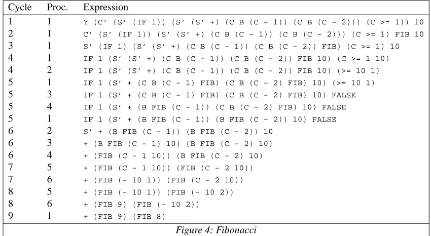
Using the nameFIBto denote this expression, and applying it to argument10, we hav e in Figure 3 the fol-lowing reduction sequences. Each line denotes the expression after one reduction step, and the symbols in the first and second columns respectively indicate the machine "cycle" and the identity of the processor which performs the reduction.

Cycle Proc. Expression

1 1 Y (C’ (S’ (IF 1)) (S’ (S’ +) (C B (C - 1)) (C B (C - 2))) (C >= 1)) 10

2 1 C’ (S’ (IF 1)) (S’ (S’ +) (C B (C - 1)) (C B (C - 2))) (C >= 1) FIB 10

3 1 S’ (IF 1) (S’ (S’ +) (C B (C - 1)) (C B (C - 2)) FIB) (C >= 1) 10

4 1 IF 1 (S’ (S’ +) (C B (C - 1)) (C B (C - 2)) FIB 10) (C >= 1 10)

4 2 IF 1 (S’ (S’ +) (C B (C - 1)) (C B (C - 2)) FIB 10) (>= 10 1)

5 1 IF 1 (S’ + (C B (C - 1) FIB) (C B (C - 2) FIB) 10) (>= 10 1)

5 3 IF 1 (S’ + (C B (C - 1) FIB) (C B (C - 2) FIB) 10) FALSE

5 4 IF 1 (S’ + (B FIB (C - 1)) (C B (C - 2) FIB) 10) FALSE

5 1 IF 1 (S’ + (B FIB (C - 1)) (B FIB (C - 2)) 10) FALSE

6 2 S’ + (B FIB (C - 1)) (B FIB (C - 2)) 10

6 3 + (B FIB (C - 1) 10) (B FIB (C - 2) 10)

6 4 + (FIB (C - 1 10)) (B FIB (C - 2) 10)

7 5 + (FIB (C - 1 10)) (FIB (C - 2 10))

7 6 + (FIB (- 10 1)) (FIB (C - 2 10))

8 5 + (FIB (- 10 1)) (FIB (- 10 2))

8 6 + (FIB 9) (FIB (- 10 2))

9 1 + (FIB 9) (FIB 8)

Figure 4: Fibonacci

Now, the first three cycles can be performed beforeFIBhas been given argument 10. Recursive calls can therefore take place in parallel, reducing the number of cycles from 9 to 6. The behaviour of this function when allowed unlimited processors is indeed 6n+O(1) cycles to evaluatefib n.

5.2. Explicit Parallelism

In order to introduce parallelism explicitly into the Fibonacci function, we use the PAR combinator, as defined above. The lambda expression we then have is:

Y λfib λn IF 1 ((λx PAR x (+ (fib (- n 1)) x)) (fib (-n 2))) (>= n 1)

This lambda expression is slightly larger than the previous one, and more combinators will be introduced by the abstraction algorithm. By a similar analysis to that in Figure 3, 17 cycles are required for each level of recursion, assuming that sufficient processors are available.

5.3. Analysis

Much of the saturation parallelism is redundant. For instance, the two arms of the IF will always be spawned, and whenfibis given small arguments, there is significant redundant computation here. Also, some of the spawned processes are very short-lived (for instance, those numbered 2 and 6 in the table above). It can be argued that the communication costs for such processes make their creation and destruc-tion undesirable. We conclude that explicit parallelism gives an acceptably efficient allocadestruc-tion of tasks to processors in this particular case, giv en the set of combinators we have elected to use.

6. Test Programs

In this section we present the results of running several programs under both strategies. The examples have been chosen so that each has significant divide-and-conquer parallelism inherent within it.

6.1. Divide-and-Conquer

6.2. Lists

The primitive functions for the list processing model are:

(i) []is the empty list.

(ii) singleton x(or alternatively[x]) is the list which contains a single elementx.

(iii) concatenate s t(or alternativelys++t) is the list formed by concatenating the listssandt.

(iv) split sis a pair of lists obtained by partitioning the listsinto two parts. It is defined only ifs con-tains at least two elements. Both lists returned are non-empty. split sis defined bysplit (concate-nate s t) = (s, t)

(v) length s(or alternatively#s) is the number of elements ofs.

(vi) element sis the only element present in the singleton lists. This function is undefined for lists con-taining more or less than one element.

Note that we model lists with++as a primitive list constructor, rather thancons.

The examples described in the following section all have natural opportunities to introduce parallelism. Those functions which employ lists in their definitions are assumed to use the divide-and-conquer list paradigm described above, where the trees implementing those lists are balanced.

6.3. Test Examples

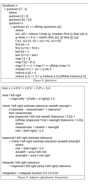
Each of the examples we used is presented here in pseudocode. The actual programs were hand-coded in FLIC. The first three have been specified as functions which take an integer argument and would be expected to exhibit time of execution linear in their argument. The fourth, quicksort, should have time quadratic in its argument. The fifth, adaptive quadrature integration, similar to an example in [4] , takes no arguments.

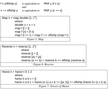
In the following examples, the annotationoffshiphas been used instead ofPARto make the code more eas-ily intelligible, where

f x (offship y) is equivalent to PAR y (f x y)

and

x ++ offship y is equivalent to PAR y (x ++ y)

Map n = map double [1..2n] where

double x = x + x map f [] = [] map f [x] = [f x]

map f (l ++ r) = map f l ++ offship (map f r) Figure 5: Map

Reverse n = reverse [1..2n] where reverse [] = [] reverse [a] = [a]

reverse (a ++ b) = reverse b ++ offship (reverse a) Figure 6: Reverse

Hanoi n = hanoi n 0 1 2 where

hanoi 0 a b c = []

Quicksor t n = quicksor t [2n..1]

where

quicksor t [] = [] quicksor t [n] = [n] quicksor t s

= quicksor t a1 ++ offship (quicksor t a2) where

(a1, a2) = reduce f (map (g (median (first s) (last s))) s) g medn x = if (x > medn) then ([x], []) else ([], [x]) f (s1, s2) (t1, t2) = (s1++t1, s2++t2)

first [n] = n first (s++t) = first s last [n] = n last (s++t) = last t map f [] = [] map f [x] = [f x]

map f (l ++ r) = map f l ++ offship (map f r) median m n = (m + n) div 2

reduce p [n] = n

reduce p (s ++ t) = p (reduce p s) (offship (reduce p t)) Figure 8: Quicksort

func x = 4.0*x3+ 3.0*x2+ 2.0*x + 5.0

area f left right

= (right-left) * ((f left) + (f right))/ 2.0

check f left right estimate tolerance newleft newr ight = if(estimate−newestimate)2< tolerance2

then newestimate

else (trapezoid f left mid newleft (tolerance / 2.0)) + (offship (trapezoid f mid r newr ight (tolerance / 2.0))) where

newestimate = newleft + newr ight mid = (left+right) / 2.0

trapezoid f left right estimate tolerance

= check f left right estimate tolerance arealeft arearight where

mid = (left+right) / 2.0 arealeft = area f left mid arear ight = area f mid right

integrate f left right tolerance

= trapezoid f left right (area f left right) tolerance

Integration = integrate function 0.0 2.0 0.01 Figure 9: Adaptive Quadrature Integration

7. Results

7.1. Maximum Speedup

We look first at the relation between the maximum possible speedup (as measured by saturation paral-lelism), and that produced by introducing explicit parallelism. For the purposes of this section, we assume an unbounded set of processors.

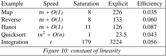
Figure 10 contains statistics relating to the execution time (measured in cycles) of the programs detailed above. Column 2 gives the actual time for the program to run (n, where appropriate, is the argument to the function). Columns 3 and 4 detail the value of t (from column 2) for the two strategies. The final column gives the ratio of columns 3 and 4, and represents the fraction of the available parallelism utilised by the "explicit" strategy.

Example Speed Saturation Explicit Efficiency

Map tn + O(1) 8 226 0.035

Reverse tn + O(1) 8 133 0.060

Hanoi tn + O(1) 11 126 0.087

Quicksort tn2+ O(n) 1 23.5 0.043

Integration t 179 3224 0.056

Figure 10: constant of linearity

A combinator expression derived from a lambda expression will, by definition, contain a number of combi-nators together with other operators mentioned in the lambda expression. In order to evaluate the expres-sion, some or all of the combinators and operators will, at some time during the evaluation, be presented with their required number of arguments. As an expression evaluates, sub-expressions will be created which can therefore be reduced concurrently (for instance, after anScombinator has been fired).

The principal reason for the high speed of saturation parallelism is the detection of all of these concurrent sub-expressions. When parallelism is explicitly described, only some of the processes which can be evalu-ated in parallel are in fact offshipped.

Our results indicate that a speedup typically of more than an order of magnitude can be accomplished by successfully detecting such sub-expressions, compared to the inherent divide-and-conquer parallelism in the original functional program. It will be apparent that many of the sub-expressions will have a very short lifetime, and therefore such parallelism could only be usefully captured on an architecture with small pro-cess creation and communication overheads.

Suppose, on the other hand, we had an implementation where our functional program is coded so that the defined functions are implemented as basic operators in their own right. Then we would expect no such extra parallelism to exist. The speedup effected by saturation parallelism is a feature of the granularity of the combinators and operators to which the functional program is compiled.

7.2. Utilisation of a Fixed Processor Set

We now look at the performance given a fixed set of processors. We use two measures. Firstly speedup, namely

lazy_reduction_steps / cycles

(where lazy_reduction_steps is the number of reductions where pure lazy evaluation is performed on a sin-gle processor) and secondly "efficiency", being

number of processors×time taken

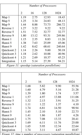
7.2.1. Saturation Parallelism

Number of Processors

2 16 128 1024

Map 1 1.19 2.75 12.93 18.43

Map 5 1.25 3.34 24.83 48.13

Map 9 1.44 8.88 73.73 286.72

Reverse 1 1.27 3.22 9.22 9.22

Reverse 5 1.51 7.52 32.77 32.77 Reverse 9 1.80 13.12 93.31 249.86

Hanoi 1 1.15 2.35 8.83 11.26

Hanoi 5 1.38 7.63 25.09 45.06

Hanoi 9 1.42 8.62 68.61 240.64 Quicksort 2 1.14 2.26 9.60 50.18 Quicksort 3 1.18 2.62 10.88 40.96 Quicksort 4 1.21 2.69 10.37 45.23 Integration 1.15 5.14 27.39 94.21

Figure 11: speedup (saturation parallelism)

Number of Processors

2 16 128 1024

Map 1 1.68 5.82 9.90 55.56

Map 5 1.60 4.79 5.16 21.28

Map 9 1.39 1.80 1.74 3.57

Reverse 1 1.57 4.97 13.88 111.06

Reverse 5 1.32 2.13 3.91 31.25

Reverse 9 1.11 1.22 1.37 4.10

Hanoi 1 1.74 6.81 14.50 90.94

Hanoi 5 1.45 2.10 5.10 22.73

Hanoi 9 1.41 1.86 1.87 4.26

Quicksort 2 1.75 7.08 13.33 20.41

Quicksort 3 1.69 6.11 11.76 25.00

Quicksort 4 1.65 5.95 12.34 22.64

Integration 1.74 3.11 4.67 10.87

Figure 12: time×number of processors (saturation parallelism)

With the saturation strategy, and where the size of problem being solved is sufficiently large, speedup is roughly half the number of processors employed. In other cases, the speedup factor is typically 20% of the number of processors available.

For the first three functions, where the number of steps necessary fully to evaluate the functions are small, the amount of available speculative parallelism is also small, and the parallel efficiency is high. Quicksort, however, requires a relatively large number of reduction steps, and there is ample opportunity for specula-tive parallelism. We therefore, not surprisingly, find that a much greater proportion of the processors are at any time engaged on evaluating unrequired sections of the graph.

For the function Reverse, we see identical speedups when 128 and 1024 processors are used, for arguments 1 and 5. These indicate that at most 128 processors were required.

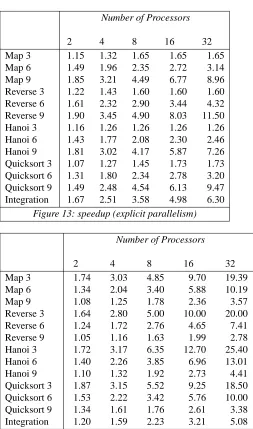
7.2.2. Explicit Parallelism

Number of Processors

2 4 8 16 32

Map 3 1.15 1.32 1.65 1.65 1.65

Map 6 1.49 1.96 2.35 2.72 3.14

Map 9 1.85 3.21 4.49 6.77 8.96

Reverse 3 1.22 1.43 1.60 1.60 1.60 Reverse 6 1.61 2.32 2.90 3.44 4.32 Reverse 9 1.90 3.45 4.90 8.03 11.50 Hanoi 3 1.16 1.26 1.26 1.26 1.26 Hanoi 6 1.43 1.77 2.08 2.30 2.46 Hanoi 9 1.81 3.02 4.17 5.87 7.26 Quicksort 3 1.07 1.27 1.45 1.73 1.73 Quicksort 6 1.31 1.80 2.34 2.78 3.20 Quicksort 9 1.49 2.48 4.54 6.13 9.47 Integration 1.67 2.51 3.58 4.98 6.30

Figure 13: speedup (explicit parallelism)

Number of Processors

2 4 8 16 32

Map 3 1.74 3.03 4.85 9.70 19.39

Map 6 1.34 2.04 3.40 5.88 10.19

Map 9 1.08 1.25 1.78 2.36 3.57

Reverse 3 1.64 2.80 5.00 10.00 20.00

Reverse 6 1.24 1.72 2.76 4.65 7.41

Reverse 9 1.05 1.16 1.63 1.99 2.78

Hanoi 3 1.72 3.17 6.35 12.70 25.40

Hanoi 6 1.40 2.26 3.85 6.96 13.01

Hanoi 9 1.10 1.32 1.92 2.73 4.41

Quicksort 3 1.87 3.15 5.52 9.25 18.50 Quicksort 6 1.53 2.22 3.42 5.76 10.00 Quicksort 9 1.34 1.61 1.76 2.61 3.38 Integration 1.20 1.59 2.23 3.21 5.08 Figure 14: time×number of processors (explicit parallelism)

With explicit parallelism, we would expect poor performance when the number of processors exceeds the available parallelism in the program. This is indeed the case. However, with relatively few processors, par-allel efficiency is high.

We obtain a speedup of typically 50% of the number of processors utilised. These figures can be compared with those obtained in [9] where Hudak and Goldberg report processor utilisation and speedup for a divide-and-conquer factorial on a distributed memory machine. A direct comparison cannot be made, for two rea-sons; they use a metric which includes communication costs for their simulated machine configured as a torus with up to 128 processors, and their algorithm for offshipping processes is simply the divide-and-conquer paradigm. Their heuristic produces a speedup factor typically 50% of the number of processors used. For our simulated machine, when the size of the problem being evaluated is large compared to the number of available processors, and where the problem naturally allows divide-and-conquer parallelism, we also obtain a speedup of around 50% of the number of processors utilised.

speculative Possible processes, and the speedup factor, which will always be at least 1, will be a measure of the efficiency with which ones offshipment algorithm accurately detects the correct subgraphs to evaluate in parallel.

8. Conclusions

We hav e examined combinator graphs derived from a number of benchmark programs, and obtained experi-mental results relating to running the program on a parallel machine. Our aim was to compare the number of parallelism opportunities and the idealized speedup factors when using various different strategies for introducing parallel evaluation. Many problems lend themselves naturally to divide-and-conquer paral-lelism. We hav e assumed that the problems are sufficiently large to ensure efficient utilization of our machine.

We hav e demonstrated that by using a "fine-grained" set of combinators one can compensate for the granu-larity of the operators used, and the consequent large number of basic reduction steps needed to evaluate a function, by employing massive parallelism. We hav e also confirmed that explicitly introducing divide-and-conquer parallelism with a small number of processors, and using the same machine, enables a speedup approaching linear in the number of processors used. Our machine provides a vehicle for modelling paral-lelism at both small and large scale.

Our results show that there is potentially a large amount of parallelism present in functional programs writ-ten in the divide-and-conquer style, but the problem size must be larger than the number of processors if good speedups are to be possible. As we have ignored the overheads of process creation and interprocessor communication, our figures are essentially upper bounds on the parallelism that can be achieved in this way. Nev ertheless, the explicit divide-and-conquer parallelism is large-grain parallelism, particularly in the earlier stages of the division part of divide-and-conquer, and not likely to be much affected by overheads. On the other hand, the extra parallelism obtained with saturation parallelism is typically fine-grain paral-lelism, and probably realisable only if process creation overheads are very small indeed.

The present analysis is applicable only to shared-memory architectures. Further work remains to be done on using a similar approach for distributed memory architectures, and on larger and more realistic applica-tions using the divide-and-conquer paradigm.

References

1. L. Acker and D. Miranker, “On Parallel Divide-and-Conquer,” Report TR-91-27, Department of Computer Sciences, University of Texas at Austin, Austin, TX (1991).

2. T.H. Axford and M.S. Joy, “List Processing Primitives for Parallel Computation,” Computer Lan-guages, 19, 1, pp. 1-17 (1993).

3. H.B. Curry, W. Craig, and R. Feys, Combinatory Logic, volume 1, North-Holland, Amsterdam, NL (1958).

4. M.I. Greenberg, “An Investigation into Architectures for a Parallel Packet Reduction Machine,” Tech-nical Report UMCS-89-1, Department of Computer Science, University of Manchester, Manchester, UK (1989). PhD Thesis.

5. P.H. Hartel, “Performance of Lazy Combinator Graph Reduction,” Software - Practice and Experi-ence, 21, 3, pp. 299-329 (1991). Also Report D-27, Fakulteit Wiskunde en Informatika, Universiteit van Amsterdam (1989).

6. W.D. Hillis and G.L. Steele, “Data Parallel Algorithms,” Communications of the ACM, 29, 12, pp. 1170-1183 (1986).

7. G. Hogen, A. Kindler, and R. Loogen, “Automatic Parallelization of Lazy Functional Programs” in ESOP’92 - 4th European Symposium on Programming, Rennes, France, ed. B. Krieg-Brückner, pp. 254-268, Springer-Verlag, Berlin, DE (1992). Lecture Notes in Computer Science 582.

8. P.R. Hudak, “Conception, Evolution, and Application of Functional Programming Languages,” ACM Computing Surveys, 21, 3, pp. 359-411 (1989).

10. P.R. Hudak and B. Goldberg, “Serial Combinators: "Optimal" Grains of Parallelism” in Functional Programming Languages and Computer Architecture, ed. J.-P. Jouannaud, pp. 382-399, Springer-Verlag, Berlin, DE (1985). Lecture Notes in Computer Science 201; ISBN 3-540-15975-4; Proceed-ings of. Conference at Nancy.

11. R.J.M. Hughes, “Super-Combinators” in Conference Record of the 1980 LISP Conference, Stanford, CA, pp. 1-11, ACM, New York (1982).

12. M.S. Joy and T.H. Axford, “GCODE: A Revised Standard Graphical Representation for Functional Programs,” ACM SIGPLAN Notices, 26, 1, pp. 133-139 (1991). Also Research Report 159, Depart-ment of Computer Science, University of Warwick, Coventry (1990) and Research Report CSR-90-9, School of Computer Science, University of Birmingham (1990).

13. J.R. Kennaway and M.R. Sleep, “Director Strings as Combinators,” ACM Transactions on Program-ming Languages and Systems, 10, 4, pp. 602-626 (1988). Also University of East Anglia Report SYS-C87-06.

14. P.W.M. Koopman, M.C.J.D van Eekelen, and M.J. Plasmeijer, “Operational Machine Specification in a Functional Programming Language,” Technical Report no. 90-21, Department of Informatics, University of Nijmegen, Nijmegen, NL (1990).

15. K. Noshita and T. Hikita, The BC-Chain Method for Representing Combinators in Linear Space, Department of Computer Science, Denkitusin University, Tokyo, JP (1985).

16. S.L. Peyton Jones, “Parallel Implementations of Functional Programming Languages,” The Com-puter Journal, 32, 2, pp. 175-186 (1989).

17. S.L. Peyton Jones and M.S. Joy, “FLIC - a Functional Language Intermediate Code,” Research Report 148, Department of Computer Science, University of Warwick, Coventry, UK (1989). Revised 1990. Previous version appeared as Internal Note 2048, Department of Computer Science, University College London (1987).

18. P. Roe, “Some Ideas on Parallel Functional Programming” in Functional Programming: Proceedings of the 1989 Glasgow Workshop, 21-23 August 1989, ed. K. Davis and R.J.M. Hughes, pp. 338-352, Springer-Verlag, London, UK (1990). British Computer Society Workshops in Computing Series; ISBN 3-540-19609-9.

19. H. Seidl and R. Wilhelm, “Probabilistic Load Balancing for Parallel Graph Reduction” in Proceed-ings IEE Region 10 Conference, pp. 879-884, IEEE, New York (1989).

20. D.A. Turner, “A New Implementation Technique for Applicative Languages,” Software - Practice and Experience, 9, pp. 31-49 (1979).