warwick.ac.uk/lib-publications
A Thesis Submitted for the Degree of PhD at the University of Warwick
Permanent WRAP URL:
http://wrap.warwick.ac.uk/130616
Copyright and reuse:
This thesis is made available online and is protected by original copyright.
Please scroll down to view the document itself.
Please refer to the repository record for this item for information to help you to cite it.
Our policy information is available from the repository home page.
"S
Quantitative Digital Image Processing in
Fringe Analysis and Particle Image
Velocimetry ( P IV )
Volume I
Thomas Richard Judge
Department of Engineering,
University of Warwick
This thesis is submitted for the degree of
Doctor of Philosophy
July 22, 1992
Declaration
This thesis is presented in accordance with the regulations for the degree of Doctor of Philosophy. It has been composed by myself and has not been submitted in any previous application for any degree. The work described in this thesis has been done by myself except where stated otherwise.
Thomas Richard Judge
Acknowledgements
I would like to give special thanks to Dr. Peter Bryanston-Cross, my supervisor, for his constant support and advice during the past three years. I would like to acknowledge the help and support of the other members of our research team; Dr. David Towers, Cathy Towers and Quan Chenggen.
I would like to thank Dr. Alan Gibbons and Darren Kerbyson for advice concerning parallel approaches to the minimum spanning tree problem.
I would also like to thank those who aided in proof reading this thesis; Louise Auchterlonie, Kay Garbett, Ruth Judge, Marcelo Funes-Gallanzi, Tim Pearce and Darren Kerbyson.
Thomas Richard Judge
Abstract
This thesis concerns the application of Quantitative Digital Image Pro cessing to some problems in the domain of Optical Engineering. The appli cations addressed are those o f automatic two dimensional phase unwrapping and the analysis of images from high speed particle image displacement ve- locimetry.
T h e first application involves subdivision of the two dimensional image of a wrapped phase map into small two dimensional areas or tiles, which are unwrapped individually, in order that discontinuities may be localised to small areas. In this case the discontinuities have a contained effect on the unwrapped phase solution.
T h e concept of minimum spanning trees, from Graph Theory, is employed to minimise the effect of such local discontinuities by computation of an un wrapping path which avoids areas likely to be discontinuous in a probabilistic manner. This approach is implemented over two hierarchical levels, the first level identifying pixel level discontinuities such as spike noise, the second ad dressing larger scale discontinuities which may not be detected by pixel level comparisons, but which can be detected by comparison of the local solutions of image areas larger than the pixel.
Contents
1 Introduction: Optical Engineering and Image Processing 19
1.1 Optical Engineering... 19
1.2 Digital Image P ro ce s s in g ... 21
2 Fringe Analysis 25 2.1 In trodu ction ... 25
2.1.1 In te rfe re n ce ... 26
2.1.1.1 A Note on N o t a t i o n ...27
2.1.1.2 Light as a Transverse W a v e ... 27
2.1.1.3 The Interference of Light Waves as Scalars . . 29
2.1.1.4 Conditions for Interference... 30
2.1.2 Producing Fringe P a tte r n s ... 31
2.1.3 Example From Real Tim e Holographic Interferometry . 35 2.1.4 A p p lica tion s... 35
2.1.5 History O f Fringe A n a ly s is ... 37
2.2 The Fringe Analysis Problem ... 38
2.3 The Analysis O f A Conventional Interferogram By Fringe Track ing ...43
2.3.1 Problems Associated W ith Fringe Tracking In Com pleting The Interferogram A n a l y s is ...44
2.4 Electronic And Quasi H eterodyn ing... 46
2.4.1 Electronic H e te ro d y n in g ...46
2.4.2 Quasi-Heterodyning... 49
2.5 The Fourier Transform T e c h n iq u e ... 53
2.6 Phase Unwrapping A lgorith m s...62
2.6.1 The Phase Fringe Counting/Scanning Approach To Phase
U nw rappin g... 62
2.6.2 Cellular-automata Method for Phase Unwrapping . . . 63
2.6.2.1 Detecting Possible Inconsistencies...64
2.6.2.2 Two-Dimensional Algorithm Description . . . 65
2.6.2.3 Cellular-automata C o n clu s io n ... 66
2.6.2.4 Modification to Original Cellular Automata A lg o rith m ... 68
2.6.3 Berlin Development of Minimum Spanning Tree Method 69 2.6.3.1 The Berlin Pixel Level Minimum Spanning Tree A lg o r ith m ... 70
2.6.3.2 Conclusion to the Berlin Pixel Level Mini mum Spanning Tree A lg o r it h m ... 70
2.6.4 Noise-immune Cut Methods of Phase Unwrapping . . . 71
2.6.4.1 Cut Method C o n c lu s io n ... 76
2.6.5 Phase Unwrapping by R e g io n s... 76
2.6.5.1 Region Method Conclusion ... 78
2.6.6 Phase Unwrapping Using a Priori Knowledge about the Band Limits of a F u n ctio n ... 78
2.6.6.1 The Band Limited Phase Unwrapping Algo rithm ...81
2.6.6.2 Band Limited Phase Unwrapping Algorithm Conclusion ... 81
2.7 C on clusion ... 81
3 The Minimum Spanning Tree Approach to Phase Unwrap ping 89 3.1 In trodu ction ...89
3.1.1 The Processing O b j e c t i v e ... 90
3.1.2 The Processing P r o b l e m ... 91
3.2 Tests for Low Modulation and Absence o f C a r r ie r ... 92
3.3 Examples of Discontinuity T y p e s ... 94
3.3.1 Aliasing I n d u c e d ...94
3.3.2 Hole in O b ject ...94
3.3.3 Absence of C a r r i e r ... 94
3.4 Adoption O f The MST Tiling Method ... 94
3.5 Graphs in Graph T h e o r y ...101
3.5.1 The Concept o f Connectedness ... 101
3.5.2 T r e e s ... 103
3.5.3 Minimum Spanning T r e e s ... 103
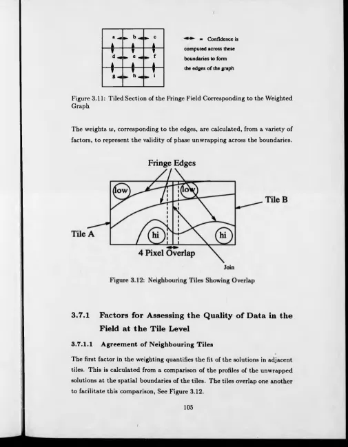
3.6 Hierarchical Phase Unwrapping Using Minimum Spanning Trees 104 3.7 High Level Phase Unwrapping, Connection o f Unwrapped Tiles 104 3.7.1 Factors for Assessing the Quality of Data in the Field at the Tile L e v e l ...105
3.7.1.1 Agreement of Neighbouring T i l e s ...105
3.7.1.2 Points of Low M o d u la tio n ... 106
3.7.1.3 Fringe D e n s i t y ... 106
3.7.1.4 Fringe Edge Termination P o in ts ... 106
3.7.1.5 M e t r i c s ... 109
3.7.2 The Minimum Spanning Tree A lg o r it h m ...110
3.7.3 Selection of an Appropriate Tile S i z e ... 112
3.8 Low Level Phase Unwrapping, Pixel to P i x e l ...116
3.8.1 The Calculation of Edge Weights at the Pixel Level . . 117
3.8.2 The Interaction of Tile Level Phase Unwrapping with the Pixel L e v e l ... 119
3.9 Examples o f Tile Level Phase U n w ra p p in g ...122
3.9.1 FFT Example o f Tile Level Phase Unwrapping...122
3.9.2 Phase Stepping Example o f Tile Level Phase Unwrappingl32 3.10 C on clu sion ...138
4 Image Capture and Processing 149 4.1 The CCD C am era...149
4.2 Capturing the Image of a S c e n e ...152
4.2.1 The Effect o f Intensity Quantization ... 153
4.3 An Experiment to Investigate the Distribution of Noise in a Particular Camera/Digitiser P a i r ... 158
4.3.1 Effect of the Camera Response Upon the Accuracy of Fringe Analysis Techniques... 165
4.3.2 Image Data F orm a t...166
4.4 Spatial Smoothing ... 166
4.4.1 Discrete Linear O p e ra to r...167
4.4.2 Nonlinear O p e ra to r...168
4.4.2.1 Median F i l t e r s ...169
4.4.2.2 Median Filter P roperties...170
4.5 Example of Smoothing on a Speckle I m a g e ... 171
4.5.1 Speckle ... 171
4.5.2 Electronic Speckle Patterns ...172
4.6 Edge D e t e c t i o n ...175
4.7 Industrial Requirements for a Fringe Analysis S y s t e m ...183
4.8 System Development by Other Researchers in Fringe Analysis 187 4.9 The Development Process for the FRAN Fringe Analysis System 189 4.10 High Speed Sequential M icroprocessors... 190
4.11 Parallel P r o c e s s in g ...191
4.12 Fringe Analysis in P a r a lle l...193
4.13 Parallel Minimum Spanning Tree Algorithm for Phase Un wrapping and its Im p lem en tation ... 196
4.14 C o n clu s io n ... 200
5 Example Fringe Analysis Applications 205 5.1 In tro d u ctio n ... 205
5.2 Deformation Measurement of a Metal D i s c ... 205
5.3 Introduction to Disc D e fo rm a tio n ...206
5.4 T h e o r y ... 207
5.4.1 Direct Deformation Measurement o f a D i s c ...207
5.4.2 Objective of Holographic Carrier Fringe Technique . . 207
5.5 Image Processing T e c h n iq u e ... 208
5.5.1 Windowing to Isolate a Side L o b e ... 208
5.6 Experimental Description and R esults... 209
5.6.1 Experimental S e t - u p ... 209
5.6.2 Correction for the Non-linearity o f the Carrier Fringes . 211 5.6.3 Results and E valuation... 213
5.7 Conclusion of Disc Deformation M e a su re m e n t... 225
5.8 Holographic Flow V is u a lis a tio n ... 226 5.9 Analysis of the Modes of Vibration o f a Vibrating Board by
Phase S t e p p in g ...231 5.10 Soldering Iron, Aliasing on An Object In The F i e l d ... 239 5.11 C on clu sion ... 253 6 P a rtic le Im a g e D is p la c e m e n t V e lo c im e t r y 256 6.1 In trod u ction ... 256 6.2 History of Particle Image Displacement V elocim etry... 263 6.3 Processing M e th o d s ...264
6.3.1 Two Dimensional Correlation and Two-Dimensional Spectrum Analysis of Young’s Fringe Pattern ... 265 6.4 Initial Semi-Automatic Data Reduction System for Transonic
PIDV via Spatial P a irin g ... 270 6.5 Improved Spatial Pairing PIDV Analysis S ystem ... 278
6.5.1 The Problem of Ambiguous Pairing and Comparison of Particle Positions ...280 6.6 Example of PIDV Analysis by 2D Autocorrelation Technique
on a Single Pair of P a r t ic le s ...283 6.7 The 2D Autocorrelation Method Applied W ith and Without
Preprocessing of the PIDV I m a g e ...287 6.8 Comparison o f Analysis by 2D Autocorrelation with that by
Spatial Pairing ... 299 6.9 Discussion o f Results for Spatial Pairing and Correlation Tech
niques ... 305 6.10 An Example o f High Speed PIDV at a Large Stand Off Dis
tance (Applied in the Transonic Wind Tunnel of A R A Bedford)307 6.11 C on clu sion ...315 7 C o n c lu s io n 319 A D o c u m e n ta tio n F or F R A N S Y S Fringe A n a ly s is S y s te m 324
A .l In trod u ction ...324 A .2 Sunview W indow In te rfa ce ... 325 A .2.1 TIF Image File D isplay...325
5
A .2.2 Pseudo Colour ...328
A .2.3 Grey S c a le ... 328
A .2.4 Printing an Image F i l e ...328
A .2.5 Reading a Project F i l e ...329
A .2.6 Creating a Project F i l e ... 329
A .2.7 Converting To Sun Raster File F o r m a t ... 330
A .2.8 Removing an Image From the C anvas... 330
A .3 The FRAN P r o g r a m ... 330
A .3.1 Project File F orm a t... 331
A .3.2 An Example Project F i l e ... 344
A .4 Converting To TIF F o rm a t... 344
A .4.1 Defaults for M k tif... 345
A .5 Converting From TIF F o r m a t ... 346
A .6 Creation of FFT Test I m a g e ... 346
A .6.1 Defaults for M k fft... 347
A .7 Displaying Information about a T IF Im a g e ... 349
A .7.1 Example Use of T i f i n f ...349
B Documentation for the Automated PIDV Image Analysis Package ( A P ) 352 B .l In trod u ction ...352
B.2 User In te r fa ce ... 353
B.3 Main M e n u ...353
B.3.1 F i l e T i f ... 353
B.3.2 File P i v ... 354
B.3.3 View T i f ... 354
B.3.4 View Vec ...355
B.3.5 Zoom I n ... 355
B.3.6 F ilte r...355
B.3.6.1 Image S ca lin g ... 356
B.3.6.2 Threshold Intensity Level for 8 Bit TIF File . 356 B.3.6.3 Particle S ize ...357
B.3.6.4 Feature S iz e ...357
List of Figures
2.1 A Transverse Wave Travelling in the Z D i r e c t i o n ... 27 2.2 Disturbance Resolved into Components along Tw o M utu
ally Perpendicular A x e s ... 28 2.3 Twym an and Green’s In terferom eter...32 2.4 The Interference of a Plane and Perturbed Wavefront, (a)
The Tw o Wave Fronts, (b) The Interference Fringe Pattern Generated. ( The intensity profile of the fringes generated is sinusoidal ) ... 33 2.5 Example Wrapped M a p ...40 2.6 Relationship o f Elements in Sector of Fringe Analysis C on
sidered ... 42 2.7 Example Problem in the Determination of Fringe Orders in
a Discontinuous F i e l d ...45 2.8 Heterodyned Twyman and Green In te r fe r o m e te r... 47 2.9 Interferometer Used in Q u a si-H eterod y n in g...50 2.10 Computer Generated Example o f Interferogram ( The Sub
ject Simulated is a Circular Disc with Pressure Applied at its Centre to Induce Deformation ) ... 54 2.11 Computer Generated Example of Interferogram ( The Sub
ject Simulated is a Tilted Flat Plate ) ... 56 2.12 Computer Generated Example of Interferogram ( The Sub
ject Simulated is a Centrally Deformed Plate which has been Tilted between Exposures ) ... 57 2.13 Real Holographic Interferogram of Centrally Deformed Plate 58 2.14 Separated Spectra o f Fringe P a t t e r n ... 59 2.15 One o f the Side Lobes Translated to the Origin . . . 60
8
2.16 2 by 2 Pixel, Path Consistency Check ... 65
2.17 A Positive Residual... 72
2.18 Two Alternative Pixel Paths for Unwrapping the Phase at Data Point x l, y l ...73
2.19 Example Cut Made Between T w o Discontinuity Sources s = +1 and s = - 1 ... 75
2.20 Field Divided into R egions... 77
3.1 Example of Aliasing Induced Discontinuity, (Original Inter-fe r o g r a m )... 95
3.2 Example of Aliasing Induced Discontinuity, (Wrapped Phase Map by FFT M e t h o d ) ...96
3.3 Example of Discontinuity Introduced by Hole in O bject, (Electronic Speckle Interferogram after Prefiltering)... 97
3.4 Example of Discontinuity Introduced by Hole in O bject, (Wrapped Phase Map by Phase Stepping with 3 Images) . . 98
3.5 Example of Discontinuity Introduced by Absence o f Carrier, (Original Interferogram )...99
3.6 Example of Discontinuity Introduced by Absence o f Carrier, (Wrapped Phase Map by FFT M e t h o d ) ... 100
3.7 Example of a G r a p h ... 102
3.8 A Disconnected G r a p h ... 102
3.9 An Example of a T r e e ... 103
3.10 A Minimum Spanning Tree of the Weighted G r a p h ...104
3.11 Tiled Section of the Fringe Field Corresponding to the Weighted G r a p h ... 105
3.12 Neighbouring Tiles Showing O v e r l a p ...105
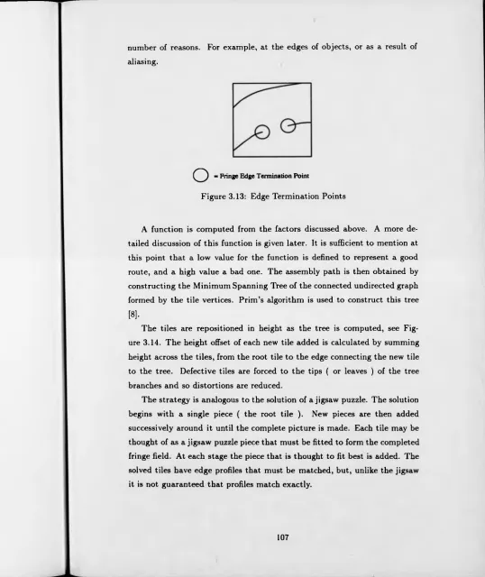
3.13 Edge Termination Poin ts...107
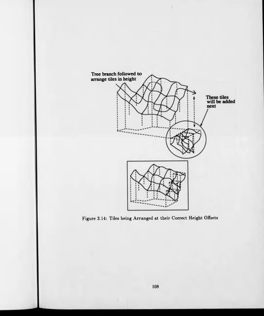
3.14 Tiles being Arranged at their Correct Height Offsets . . . . 108
3.15 Selection of Tile Size: Tile with One Broken Fringe Edge . . 112
3.16 Selection of Tile Size: Tile with T w o Broken Fringe Edges . 114 3.17 Illustration of Effect of Tile Size ... 115
3.18 Pixel Level, Computation of Edge Weights. Weights are Computed over Four Pixels for Each Pair ...118
3.19 Mountaineer Analogy in Pixel Level Phase Unwrapping . . . 119 3.20 Interaction of Tile Level Phase Unwrapping with the Pixel
L e v e l... 120 3.21 Pixel Level Phase Unwrap Circumnavigates Phase Distortion 121 3.22 Tile Level Phase Unwrap Circumnavigates Smooth Area . . 121 3.23 Wrapped Phase Map for Disc Showing Problem Areas . . . 123 3.24 Points of Low Modulation for Disc ( shown in white ) . . . . 124 3.25 Weighting Factor for Disc : Agreement between Neighbour
ing T ile s ...125 3.26 Weighting Factor for Disc : Low Modulation P o in ts ... 126 3.27 Weighting Factor for Disc : Fringe Edge Termination Points 126 3.28 Weighting Factor for Disc : Points on Fringe E d g e s ... 127 3.29 Combined Weighting Factors for D is c ... 128 3.30 Edge Detection and Minimum Spanning Tile Tree for Disc . 129 3.31 Contour Plot o f Unwrapped Numerical Phase Data ( Sam
pled at Every 5th Pixel in X ) Showing Circumvention of Shadow D is c o n tin u ity ...130 3.32 Raw ESPI I m a g e ... 133 3.33 Wrapped Phase Map for Chamber Showing Problem Areas . 134 3.34 Points of Low Modulation for Chamber ( shown in white ) 135 3.35 Weighting Factor for Chamber : Agreement between Neigh
bouring T i l e s ...138 3.36 Weighting Factor for Chamber : Low Modulation Points . . 139 3.37 Weighting Factor for Chamber : Fringe Edge Termination
P o i n t s ... 139 3.38 Weighting Factor for Chamber : Points on Fringe Edges . . 140 3.39 Combined Weighting Factors for C h a m b e r ... 141 3.40 Edge Detection and Minimum Spanning Tile Tree for Cham
ber ( Includes Low Modulation Points in Grey ) ...142 3.41 Contour Plot o f Unwrapped Numerical Phase Data for Cham
ber ( Sampled at Every 5th Pixel ) Showing Circumvention of Missed Fringe E d g es...143
10
3.42 Mesh Plot of Unwrapped Numerical Phase Data for Cham ber after Post Processing via 3 by 3 Median Filter ( Sampled at Every 5th Pixel ) ... 144 3.43 Grey Scale Image of Unwrapped Numerical Phase Data for
Chamber Showing Circumvention of Missed Fringe Edges . . 145 3.44 Octagonal tiles would allow better Consistency Testing (
across diagonals ) ... 146 4.1 CCD Cells Arranged on Rectangular G r i d ... 149 4.2 ID Slice for p-type CCD C e l l ... 150 4.3 Generation of Minority Carrier Charge Packet from Incident
Illumination (1-D S l i c e ) ... 151 4.4 Input Video Signal Gain and Offset C o n t r o l ...155 4.5 Representation of Sampling the Analog Intensity Signal . . 155 4.6 Probability Density Function of Quantization Error with
Truncation ... 157 4.7 Experimental Arrangement for Camera Noise Experiment . 158 4.8 Result of Camera/Digitiser Noise Experiment, Gain 1 . . . . 162 4.9 Result of Camera/Digitiser Noise Experiment, Gain 2 . . . . 163 4.10 Result of Camera/Digitiser Noise Experiment, Gain 3 . . . . 164 4.11 Standard Deviation of Intensity Against Mean for Varying
G a in ... 164 4.12 Section of an Electronic Speckle Pattern ( Normalised In
tensity ) 172
4.13 Section of an Electronic Speckle Pattern ( After 3 X 3 A v
erage ) 173
4.14 Section of an Electronic Speckle Pattern ( After 3 X 3 Me dian ) ... 174 4.15 Illustration of Step Edge Detection using Zero Crossing o f
2nd Derivative, ( f(x) is a step function, f2(x) is a smoothed step function ) ... 178 4.16 Typical Curves for Different Edge O perators... 179 4.17 Gaussian Smoothing Kernel ( Sigma = 5 ) ... 180 4.18 Laplacian-of-a-Gaussian Smoothing Kernel ( Sigma = 5 ) . . 181
4.19 Example Wrapped Phase Map for Edge D e te ctio n ...184 4.20 Sobel Gradient Edge Detector with Adaptive Thresholding
Applied to Wrapped Phase Map, Kernel = 3 X 3 ... 185 4.21 Laplacian o f a Gaussian Edge Detection Applied to Wrapped
Phase Map, Kernel = 9 X 9 , Sigma = 1 . 0 ... 186 4.22 Mapping o f Problem to Algorithm, Algorithm to Architecture 192 5.1 Experimental Arrangement for Recording Holograms of the
Disc b y the Carrier Fringe T ech n iq u e...210 5.2 Optical and Electronic Arrangement for Reconstruction of
the Holograms ...211 5.3 Schematic Diagram for Generation of Carrier Fringes at
Slight In clin a tio n ... 212 5.4 Double-exposure Holographic Interferogram of the Centrally
Loaded D i s c ... . 214 5.5 Holographic Carrier Fringe Interferogram of the Centrally
Loaded D is c ... 215 5.6 Wrapped Phase Map for Centrally Loaded Disc, Generated
by the F F T T e ch n iq u e ...216 5.7 Normalised grey scale plot of deformation produced by un
wrapping procedure, before correction for non linearity of carrier fringes... 217 5.8 (a) Digitised intensity data of central raster in the interfer
ogram; (b ) intensity data weighted by Papoulis window. . . 218 5.9 (a) Power spectrum o f central raster from the interferogram
with carrier and deformation (the window is indicated by the dashed dot line); (b) side lobe translated by the carrier frequency to the origin position...219 5.10 3-D perspective plot o f the out of plane displacement of the
centrally loaded disc after phase unwrapping and correction. 220 5.11 Side view o f unwrapped numerical phase data... 222 5.12 Side view o f the unwrapped and corrected numerical phase
data...223
12
5.13 Comparison between the theoretical and measured deforma tion for cross section... 224 5.14 Finite Fringe Hologram of a N AC A 0012 Aerofoil at a Freestream
Mach Number of 0.8, copyright British Aerospace PLC 1991 for p u b lic a t io n ...227 5.15 Wrapped Phase Map by ID FFT Method via FRAN for
N AC A 0012 Aerofoil, copyright British Aerospace PLC 1991 for p u b lic a t io n ...228 5.16 Edge Detection and Tile Connection Tree via FRAN for
N ACA 0012 Aerofoil, copyright British Aerospace PLC 1991 for p u b lic a t io n ... 229 5.17 Grey Scale Unwrapped Phase Map by ID FFT Method via
FRAN for NACA 0012 Aerofoil, copyright British Aerospace PLC 1991 for p u b lic a t io n ... 230 5.18 Averaged Background Image for NACA 0012 Aerofoil, copy
right British Aerospace PLC 1991 for p u b lic a tio n ...232 5.19 Wrapped Phase Map by 2D FFT Method for NACA 0012
Aerofoil at a Freestream Mach, copyright British Aerospace PLC 1991 for p u b lic a t io n ... 233 5.20 Edge Detection and Tile Connection Tree via FRAN for
2D FFT Analysis o f NACA 0012 Aerofoil, copyright British Aerospace PLC 1991 for p u b lic a t io n ... 234 5.21 Contour Plot of Unwrapped Phase Map, Every 5th Pixel,
by 2D FFT Method via FRAN for NACA 0012 Aerofoil, copyright British Aerospace PLC 1991 for publication . . . 235 5.22 Mesh Plot of Unwrapped Phase Map, Every 5th Pixel, by
2D FFT Method via FRAN for NACA 0012 Aerofoil, copy right British Aerospace PLC 1991 for p u b lic a tio n ... 236 5.23 Grey Scale Unwrapped Phase Map by 2D FFT Method via
FRAN for Finite Fringe Hologram of a NACA 0012 Aerofoil, copyright British Aerospace PLC 1991 for publication . . . 237 5.24 Original Holographic Cosinusoidal Interferogram of Vibrat
ing Board after P r e filte r in g ... 240 5.25 Wrapped Fringe Field for Vibrating B o a r d ... 241
13
5.26 Low Modulation Noise ( in White ) for Vibrating Board . . 242
5.27 Edge Detection of Wrapped Fringe Field for Vibrating Board, Showing Tiles and Connection T r e e ... 243
5.28 Grey Scale Unwrapped Fringe Field for Vibrating Board . . 244
5.29 Contour Plot of Unwrapped Phase for Vibrating Board, Ev ery 5th Pixel on Long Axis ... 245
5.30 Mesh Plot o f Unwrapped Phase for Vibrating Board . . . . 246
5.31 Soldering Iron Interferogram with Carrier F rin g e s... 247
5.32 Wrapped Phase Map O f Soldering I r o n ... 248
5.33 Edge Detection and Tile Connection Tree for Soldering Iron 249 5.34 Grey Scale Plot of Solution Showing Circumvention of Dis continuities in Area of Soldering I r o n ... 250
5.35 Contour Map Of Soldering Iron S o lu t io n ...251
5.36 Mesh Plot O f Soldering Iron S olu tion ... 252
6.1 Coding Techniques for Image V e lo c im e t r y ...259
6.2 Schematic Diagram of PID V as Applied in Transonic Wind T u n n el... 259
6.3 Interrogation of a Double Exposed Transparency (a) Pro cessing in the 2-D Image Plane via Tw o Dimensional Cor-•• relation, (b) Processing by Young’s Fringe Analysis in the Fourier Transform Plane o f the Im a g e s ... 266
6.4 Efficient Use of Spatial C o r r e la tio n ...269
6.5 Initial Semi-Automatic Data Reduction System for Tran sonic P I D V ... 271
6.6 Image Captured from Original Data Reduction System show ing Two Clear Particle P a ir s ...272
6.7 Computation of Particle Centre from Bounding Box in PIDV273 6.8 Error in Measuring Velocity Vector at a Variety o f Angles . 275 6.9 Error in Vector Measurement is Greatest at 45 Degrees . . . 276
6.10 Data Reduction System Based Upon Flat Bed Scanner . . . 278
6.11 Schematic of Particle Pairs Showing an Ambiguous Pairing P r o b le m ...280
14
6.12 Schematic o f Particle Pairs, Circles Define the Maximum Distance that a Particle could have Moved, Pulse to Pulse . 280 6.13 Schematic o f Particle Pairs, Ambiguous Pairings are Deleted
and Velocities Computed for the Remaining P a ir s ... 281 6.14 Bounding Box Test to Improve Performance o f Pairing Al
gorithm ... 283 6.15 Single Pixel Pair Image ...284 6.16 Single Pixel Pair Image 2D Power Spectrum with DC Removed285 6.17 Single Pixel Pair A u to co rre la tio n ... 286 6.18 Thrust Reverser ... 288 6.19 Whole Field View of PIDV Experiment on Thrust Reverser
showing Area of Test Image in B o x ... 289 6.20 Test I m a g e ...290 6.21 Test Image 2D Power Spectrum with DC R e m o v e d ... 291 6.22 Test Image 2D Autocorrelation ( Circle Defines Maximum
Velocity 300 m / s ) ...292 6.23 Test Image after Reducing Particle Images to Single Pixels . 294 6.24 Reduced Test Image 2D Power S pectrum ...295 6.25 Reduced Test Image 2D Autocorrelation ( Circles Define
Minimum Velocity = 100 m /s and Maximum Velocity = 300 m /s ) ... 296 6.26 Contour Plot of Central Region o f Autocorrelation for Re
duced Test Im a ge... 297 6.27 Mesh Plot o f Central Region of Autocorrelation for Reduced
Test I m a g e ...298 6.28 Part of Test Image after Reducing Particle Images to Single
P i x e l s ...300 6.29 Part of Reduced Test Image 2D Power Spectrum with DC
R e m o v e d ... 301 6.30 Part of Reduced Test Image 2D Autocorrelation ( Circles
Define Minimum Velocity = 100 m /s and Maximum Veloc ity = 300 m /s ) ... 302 6.31 Contour Plot of Central Region o f Autocorrelation for Part
of Reduced Test Im a g e ... 303
15
6.32 Mesh Plot of Central Region of Autocorrelation for Part of Reduced Test I m a g e ... 304 6.33 Result o f Test Image Analysis by Spatial Analysis Superim
posed on Test I m a g e ... 306 6.34 PIDV Vector Plot For Thrust Reverser, Pulse Separation
2.0 Microseconds, Minimum Allowed Velocity = 100 m /s, Maximum Allowed Velocity = 300 m /s, Minimum Allowed Angle ( from vertical ) = 120 degrees, Maximum Allowed Angle = 1 7 0 d e g r e e s ... 308 6.35 PIDV Histogram of Velocity for Thrust R e v e r s e r ... 309 6.36 PIDV Histogram of Velocity Vector Angle for Thrust Reverser310 6.37 Scan of PIDV Print, Mach No. 0.2, Frame No. 7, 10 Mi
crosecond Pulse Separation, Model at Incidence o f 5 Degrees 311 6.38 PIDV Vector Plot Mach No. 0.2, Frame No. 7, 10 Microsec
ond Pulse Separation, Model at Incidence of 5 Degrees . . . 312 6.39 PIDV Histogram o f Velocity, Mach No. 0.2, Frame No. 7,
10 Microsecond Pulse Separation, Model at Incidence of 5 D e g r e e s ...313 6.40 PIDV Histogram o f Velocity Vector Angle, Mach No. 0.2,
Frame No. 7, 10 Microsecond Pulse Separation, M odel at Incidence of 5 D e g r e e s ...314 A .l Example FFT Image Generated By m k f f t ... 326 A .2 Sunview Window Interface to F R A N S Y S ... 327 A .3 Image Data Display in S u n v ie w ... 328 A .4 Example FFT Wrapped M a p ...334 A .5 Example FFT Edge Detection of Wrapped Map, W ith Tree A d d e d ... 335 A .6 Example FFT Unwrapped M a p ... 336 A .7 Original Intensity Data For Raster 128 ... 338 A .8 Intensity Data o f Raster 128 Weighted by Papoulis Window 339 A .9 Power Spectrum o f Scan Line and Papoulis Weighting Window339 A. 10 Translated Side L o b e ...340 A. 11 Example FFT Mesh Plot ...341
A. 12 Example FFT Contour P l o t ... 342 A. 13 Boundary E x a m p le ...343 A. 14 Example Project F ile ...344 A. 15 Example Concentric Fringe Im a ge...348 A. 16 Tifinf E x a m p le ... 350 B . l PC Screen Display for AP P a c k a g e ...353 B.2 Schematic of Particle Pairs Showing an Ambiguous Pairing
P r o b le m ... 358 B.3 Schematic of Particle Pairs, Circles Define the Maximum
Distance that a Particle could have Moved, Pulse to Pulse . 358 B.4 Schematic of Particle Pairs, Ambiguous Pairings are Deleted
and Velocities Computed for the Remaining P a ir s ... 358 B.5 Specifying Band Limits for D ir e c tio n ... 359
List of Tables
i n 160 161 161 162 4.5 Execution Times for Breuckmann’s Dedicated Software+Hardware C o m b in a t io n ... 189 4.6 Execution Times for Hardware Independent Analysis Soft
ware, on Various Processors, Using 3 Phase Stepped (512 by 512) Images, Without P refilterin g... 189 6.1 Summary o f Fourier Analysis Result for Edited Test Image . 299 6.2 Summary o f Fourier Analysis Result for Lower Left Corner
of Test I m a g e ... 299 6.3 Summary o f Spatial Pairing Analysis Result for Test Image 299 6.4 Summary o f Spatial Pairing Analysis Result for Thrust Re
verser ( Complete Field ) 307 6.5 Summary o f Spatial Pairing Analysis Result for Example
A R A T e s t ... 309 3.1 Tabular Representation o f the Weighted G r a p h ... 4.1 Goodness o f Fit Test. That is, a Comparison of the Noise
Distribution against the Normal Distribution, for Gain 1 . 4.2 Goodness o f Fit Test. That is, a Comparison o f the Noise
Distribution against the Normal Distribution, for Gain 2 . 4.3 Goodness o f Fit Test. That is, a Comparison of the Noise
Distribution against the Normal Distribution, for Gain 3 . 4.4 Summary o f Goodness o f Fit Tests, Comparing the Noise Distribution with the Normal D istrib u tion ...
18
Chapter 1
Introduction: Optical
Engineering and Image
Processing
1.1
Optical Engineering
Optical engineering is an established field; it is a generic term which covers all applications where a measurement is being made or processing performed using an optical element or aspect. It plays an ever increasing role in a wide range o f applications. This expansion has been due in part to the dis covery and rapid development o f versatile lasers covering the ultraviolet to far-infrared regions, and a parallel development of solid-state and optical materials. The introduction o f optical fibres and semiconductor lasers in communication has also stimulated the relationship between optics and com munication engineering [1]. Other important areas within optical engineering are in optical measurement, and optical diagnostics. These are respectively, quantitative and qualitative techniques. The extraction o f quantitative mea surements from optically captured data, via image processing, is the subject o f this work.
There are a number of important issues in the development of an optically based measurement technique. Firstly the nature of the parameter to be measured must be considered , then the light source, the optical components ( lens etc. ), the effect of the experimental environment, consideration of
19
the process which is to record the result, and then analysis of the recording. The subject is multidisciplinary by its nature, requiring knowledge from such areas as Physics, Mechanical Engineering and Computer Science. Physics is required to cover the theoretical aspects. Mechanical Engineering is involved in the design and development o f experiments. Computer Science is involved in the design and development of the analysis techniques and also in providing digital control of experiments.
There are several motivations for the use of optical techniques. Firstly, the properties of light make highly accurate measurement possible. Secondly, optical techniques are non-contact, which is important for many applications where a measurement would be upset by touch, or the introduction of a foreign body, for example in flow visualisation. In addition optical techniques are non-destructive.
Optically captured results ( stored either holographically, photographi cally or by video ) need further processing to yield quantitative data. Com puter Science covers the techniques used to develop the necessary algorithms, and the machine architectures upon which such algorithms could be efficiently implemented.
Historically there have been several impediments to the quantitative anal ysis of many images generated by optical techniques. In many applications quantitative analysis has had to attend the development o f low-cost high speed digital computers, the development o f low-cost imaging technology, which could be easily interfaced to such computing facilities, the develop ment o f the discipline of image processing and standard methods, and lastly the development of the specific methods of analysis required for the image types found in optical engineering.
This thesis concerns the development of a number of analysis strategies, aimed at quantitative analysis of two image subclasses in optical engineering. The first subclass being interferometric images, the second subclass being high speed images from Particle Image Displacement Velocimetry ( PIDV ). It has been necessary to apply techniques from the field of Digital Image Processing and more general computer science to achieve the ends of analysis.
There is often an interdependency between the design of the experiment and the design o f the analysis technique. In the development of the complete
system, one o f the aims is to simplify this relationship. The development of analysis techniques requires an understanding of the experiment and the devices used to capture the image data, as well as the techniques employed in analysis. There has been some direct interaction in the experiments them selves and digital control has been provided in several instances.
1.2
Digital Image Processing
Digital image processing is a relatively new field. It has experienced tremen dous growth over the past decade. There has been some development of standard algorithms for defined tasks. For example, edge detection [2]. The wider goal of computer vision, however, is to solve the ’vision problem ’ as a whole. That is in the sense of scene analysis, or robot vision, to produce a description of the scene being observed, in terms of the objects in view and their properties or at a higher level what the scene as a whole means. There has been less success in this area.
The last decade has seen an increasing effort to develop sophisticated, real-time automatic image processing systems.
The processing tasks considered in this work require the extraction and display of coded information from an image, rather than emulation o f human behaviour or image enhancement. Take the case of Interferometry. In this application an interference pattern is produced from beams of light, influ enced by a physical parameter, e.g. temperature. The interference pattern encodes the temperature information and an image processing function is needed to extract it. This is typical of many Engineering applications where images are encoded, perhaps by physical effects during an experimental pro cess. Structured light is often employed to encode information.
In pursuing the objectives of image processing, a range o f often interde pendent numerical tools are currently employed. They include signal anal ysis, geometry, linear algebra, estimation theory, statistical pattern recog nition, syntactic pattern recognition ( for image structural description ), discrete mathematics and a number o f topics often referred to under the heading of ’’ artificial intelligence” , which include knowledge representation and manipulation, constraint satisfaction, symbolic manipulation, and more
21
recently neural networks.
T he implementation requirements of image processing systems, in terms of hardware and software are substantial, particularly when "real-time” op eration is needed and the resolution o f images from video systems continues to increase, thus aggravating the problem. Processing capacity has placed a limit on the applications to which image processing might be applied. The possibility of real time response is an attractive prospect in many applica tions, particularly in Engineering, as it opens up the possibilities of human interaction with the system. This is a tremendous contrast with conventional photography, which involves time consuming wet processing.
In order to achieve high processing speeds, dedicated hardware is some times employed. This is virtually impossible to update with changing require ments. Software solutions offer flexibility against a reduced processing rate. The power of sequential processors continue to increase, and for many appli cations provide adequate solutions. Image processing and computer vision research serves as an impetus for the development of new processing architec tures, particularly parallel processing systems. Such systems offer software control and therefore retain some flexibility, although standards have been slow to emerge.
A hardware independent approach to development has been taken in this work, where possible, as the test cycle of algorithmic development has re quired flexibility. As a by product of this strategy, the Fringe Analysis Sys tem ( FRANSYS ) has becom e a portable software application.
High speed sequential processors have developed since the inception of the project, particularly RISC ( Reduced Instruction Set Computer ) processors. It is seen that for many current interferometric applications, a sequential software implementation upon such a processor is adequate, and provides a flexible upgrade path. However, it is also shown that the automated phase unwrapping algorithm, developed in this work, is extremely well suited to parallel implementation.
In the application of Particle Image Displacement Velocimetry ( PIDV ), optical processing has been employed for some time. However, with the advent of high resolution video capture devices, digital analysis methods are more appropriate as these avoid wet processing and offer the prospect o f
real time systems. Direct simulation of the optical processing methods is numerically intensive. This, together with the sparse seeding density found in high speed PID V , has prompted a search for a more informative and less numerically intensive digital analysis technique for high speed PIDV.
Bibliography
[1] F. T. S. Yu, I. C. K hoo, Principles of Optical Engineering, John Wiley Sons, Inc., 1990.
[2] R. J. Schalkoff, Digital Image Processing and Computer Vision, John Wiley & Sons, Inc., 1989.
Chapter 2
Fringe Analysis
2.1
Introduction
This work describes a new technique in the field o f Automatic Interferometric Fringe Analysis.
Reid [1] suggests that the field o f Fringe Analysis is now regarded by many as a subject in its own right, rather than as a specialism within image processing or interferometry. I believe this to be the case. If the field is viewed as an independent subject, then this has the benefit of encouraging the development o f concepts and methods which may be applied to the patterns generated by any one o f a number of optical methods. The source of the fringe pattern then has little to do with the analysis algorithm. The development described in this work is a new phase unwrapping technique, which is referred to as the Minimum Spanning Tree Tiling (M ST T) approach. This technique, in common with other methods in fringe analysis, may be applied to many types of fringe pattern, from Interferometry to Moire.
There has been an increasing interest in the automation of Fringe Analysis over the last decade. The advent of Phase Stepping [2, 3, 4, 5] and the development of FFT techniques [6, 7] has moved the emphasis in Fringe Analysis away from fringe tracking [8, 9, 10] and towards fringe counting or scanning techniques [11, 12]. One difficulty with such scanning approaches has been their susceptibility to noise.
However, several strategies have recently been proposed which exhibit noise immunity [13, 14, 16], but which have failed to address large scale
25
inconsistencies in interferograms which cannot be detected at the pixel level, such as aliasing.
The new m ethod presented forms a hierarchical noise-immune technique which addresses both spike noise and large scale discontinuities.
In order to place the work in context, it is necessary to review the concepts involved in Interferometry. For the purposes of the work described here, light is modeled in the form of scalar waves.
2.1.1
Interference
The theory of light interference, using the wave theory of light, is based on the Principle o f Superposition due to Thomas Young. The following discussion is derived from Hecht [17].
The essential aspect of a propagating wave is that it is a self-sustaining disturbance of the medium through which it travels. Imagine some such disturbance moving in a positive direction x. This disturbance, for the electromagnetic light wave, represents the magnitude of the electric or mag netic field. Since the disturbance is moving, it must be a function o f both position x and time t and can therefore be written as;
'l' = /( * ,< ) (2.1) The Principle o f Superposition states that if a wave train has a displace ment in a given direction at a specified point and time, and a second wave train independent of the first has a displacement at the same point and time, then the instantaneous resultant displacement due to the two waves is the algebraic sum of the separate displacements.
<1» = «Jr, -I- vl»2
(2.2)
The Principle of Superposition implies the absolute independence of the individual components of the resultant displacement. The term Interference is, therefore, slightly misleading as the waves do not modify each other [18].
2.1.1.1 A Note on Notation
Waves for which the profile is a sine or cosine curve are known as harmonic waves. A concise representation of harmonic waves is achieved using complex notation. For example, if is the phase, and A is the amplitude;
= i4cos(<^) (2.3) may be expressed as
® (x,< ) = # [A e <v] (2.4) or more simply, assuming that the real part is taken, as
vp(x,t) = A e ” (2.5)
2.1.1.2 Light as a Transverse Wave
[image:33.601.17.561.18.680.2]Light actually behaves like a transverse wave. That is, it has an associated plane o f vibration which is important to consider in certain applications.
Figure 2.1: A Transverse Wave Travelling in the Z Direction
A transverse wave arises when the disturbance is perpendicular to the propagation direction. Figure 2.1 depicts a transverse wave travelling in a
direction z. In this instance, the wave motion is confined to a spatially fixed plane called the plane of vibration, and the wave is said to be linearly or plane polarised. To determine the wave completely, the orientation of the plane of vibration must be specified, as well as the direction of propagation. This is equivalent to resolving the disturbance into components along two mutually perpendicular axes, both normal to z, see Figure 2.2.
[image:34.598.10.557.15.666.2]y
Figure 2.2: Disturbance Resolved into Components along Two Mutually Per pendicular Axes
The angle at which the plane of vibration is inclined is a constant, so that at any time 'I'x and differ from »I» by a multiplicative constant. The wave function of a transverse wave behaves somewhat like a vector quantity. W ith the wave moving along the z-axis;
« '(z ,< ) = ^ x (z,< )T + 4 »v(z,<)J (2.6) where, I, J are the unit base vectors in Cartesian coordinates.
A scalar harmonic plane wave, moving in the z direction, is given by the expression
#(*,<) =
Ae*k' ±wt) (2.7)where u is the angular frequency.
An appreciation o f light’s vectorial nature is important. Phenomena such as optical polarisation can readily be treated in terms of this sort of vector wave picture [17]. However, there are many instances in which it is not necessary to be concerned with the vector nature of light. In particular, if the lightwaves all propagate along the same line and share a common constant plane of vibration, they may each be described in terms o f one electric-field component. This approach leads to a simple and very useful scalar theory, which will be applied in this work.
2.1.1.3 The Interference of Light Waves as Scalars
Hecht [17] gives a derivation of the superposition of a pair o f harmonic scalar waves, and then extends the treatment to N such waves. Given two scalar light waves, overlapping in space;
E i = I?oi sin(u;< + c*i) (2.8) and
E? = E02 sin(u>< + <*2) (2.9) The resultant disturbance is the linear superposition of the waves. There fore
E = E i + E2 (2.10)
or, expanding Equations 2.8 and 2.9;
E = E oi(sinw <cosai-(-cosa;<sinQ i)-|-Eo2(sinu;<cosQ 2+cosu)i8ina2) (2.11)
If the time-dependent terms are separated out, this becomes;
29
£ = ( E 0i co sa i + £ 0 2 c o s a 2) sinwi + ( £ 0 1 sinai + ¿J02 s in a 2)cosu d (2.1 2) and since the bracketed quantities are constant in time, let
Eo cos a = £ 0 1 cos a i + £ 0 2 cos 0 2 (2.13)
and
Eo sin a = E01 sin a i + £ 0 2 sin 0 2 (2-14) The substitution above is not obvious, but it is legitimate as long as E 0
and a can be solved for. To do so, square and add Equations 2.13 and 2.14;
E 02 = £ 0 1 2 + £o2 2 + 2 £ 0 1£ 0 2 cos(a2 — a i) and divide Equation 2.14 by 2.13 to get
£ 0 1 sin ai + £ 0 2 sin a2
tan a =
—---—---£ 01 COS Ol + £ 0 2 COS 0 2
The total disturbance then becomes;
(2.15)
(2.16)
or
E = Eqcos a sin uit + E 0 sin a cos ujt (2.17)
£ = £osin(u>t + a ) (2.18) Thus a single disturbance results from the superposition of the sinusoidal waves £ 1 and £2. The composite wave is harmonic and o f the same frequency as the constituents, although its amplitude and phase are different.
2.1.1.4 Conditions for Interference
Conventional light sources produce light that is a mix o f photon wavetrains. At each illuminated point in space there is a net field that oscillates ( through roughly a million cycles ), for less than 1 0ns or so, before it changes phase.
30
This interval over which the lightwave resembles a sinusoid is a measure o f what is called its temporal coherence.
As observed from a fixed point in space, the passing lightwave appears fairly sinusoidal for some number of oscillations between abrupt changes o f phase. The corresponding spatial extent over which the light wave oscillates in a regular, predictable way is called the coherence length.
To produce a stable interference pattern, the light sources must be co herent and have the same frequency. Until the advent of the laser it was a working principle that no two individual sources could ever produce an o b servable interference pattern. The coherence tim e of lasers, however, can be appreciable ( of the order of milliseconds ), and interference via independent lasers has been detected electronically ( though not yet by the rather slow human eye ). The most common means of overcoming this problem, as we shall see, is to make one source serve to produce two coherent secondary sources. [17]
2.1.2
Producing Fringe Patterns
The fringe patterns, or interferograms, which are treated in this work are produced by the interference of light. Such patterns are highly useful as they can be used to code a variety of physical measurements.
A divided beam is used to generate an interferogram. One part of the beam is used as a phase reference, and the path of the rest o f the beam is influenced in some way. For example this could involve the latter ‘ob ject beam ’ , being reflected from an ob ject to record displacement, or passing through a translucent object to record refractive index. It is possible to decode and quantify the measurement parameter by analysis of the fringe pattern formed when the beams are recombined.
The device which controls the interference of the light beams is called an interferometer. The earliest and most widely known interferometer is the Michelson. This was the interferometer used by Michelson and Morley to explore the existence of the luminiferous aether at the end of the 19th century. The Twyman and Green interferometer, Figure 2.3, is a variation o f the Michelson.
31
There now follows a description o f the operation of the interferometer, together with examples of its use in detecting faults in a glass plate or mea suring surface deformation.
Imagine a plane wave coming from the point source 5 through the lens
O j . This wave is divided in two by the beam splitter B .
Figure 2.3: Twyman and Green’s Interferometer
One o f the divided beams is reflected back from the plane mirror M\ and the other from the mirror M2. Either beam may have its phase disturbed during its passage, and in this case, assuming the mirrors are ideal, any disturbance will be due to the glass plate under test.
The beams are reunited and brought to focus by a second lens C>2- The result may be viewed by placing the eye, or a camera, at E .
The compensator plate C is an exact duplicate of the beam-splitter, with the exception of any silvering or thin film coating. With the compensator in place, any optical path difference arises from the actual path difference. It is positioned at an angle of 45 degrees, so that B and C are parallel to each other.
If the two com bining wavefronts are plane, the plate having no defects, the result will be uniform in intensity. If there are defects in the plate, a
32
[image:38.601.11.562.19.668.2]There now follows a description of the operation of the interferometer, together with examples of its use in detecting faults in a glass plate or mea suring surface deformation.
Imagine a plane wave coming from the point source S through the lens
0\. This wave is divided in two by the beam splitter B .
M
[image:39.598.4.561.17.673.2]2
Figure 2.3: Twyman and Green’s Interferometer
One of the divided beams is reflected back from the plane mirror M\ and the other from the mirror M2. Either beam may have its phase disturbed during its passage, and in this case, assuming the mirrors are ideal, any disturbance will be due to the glass plate under test.
The beams are reunited and brought to focus by a second lens The result may be viewed by placing the eye, or a camera, at E .
The compensator plate C is an exact duplicate of the beam-splitter, with the exception of any silvering or thin film coating. With the compensator in place, any optical path difference arises from the actual path difference. It is positioned at an angle of 45 degrees, so that B and C are parallel to each other.
If the two combining wavefronts are plane, the plate having no defects, the result will be uniform in intensity. If there are defects in the plate, a
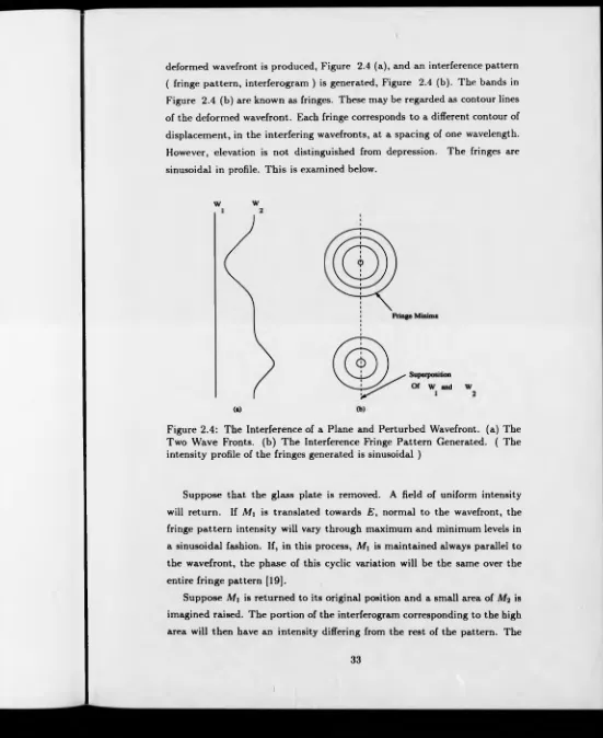
deformed wavefront is produced, Figure 2.4 (a), and an interference pattern ( fringe pattern, interferogram ) is generated, Figure 2.4 (b). The bands in Figure 2.4 (b) are known as fringes. These may be regarded as contour lines of the deformed wavefront. Each fringe corresponds to a different contour of displacement, in the interfering wavefronts, at a spacing of one wavelength. However, elevation is not distinguished from depression. The fringes are sinusoidal in profile. This is examined below.
w w
Figure 2.4: The Interference of a Plane and Perturbed Wavefront, (a) The Two Wave Fronts, (b) The Interference Fringe Pattern Generated. ( The intensity profile of the fringes generated is sinusoidal )
Suppose that the glass plate is removed. A field of uniform intensity will return. If M\ is translated towards E , normal to the wavefront, the fringe pattern intensity will vary through maximum and minimum levels in a sinusoidal fashion. If, in this process, M\ is maintained always parallel to the wavefront, the phase of this cyclic variation will be the same over the entire fringe pattern [19].
Suppose A/i is returned to its original position and a small area of is imagined raised. The portion of the interferogram corresponding to the high area will then have an intensity differing from the rest of the pattern. The
33
[image:40.606.16.567.15.689.2]exact height o f this plateau, with respect to the wavelength o f the light used, will determine its intensity in the interferogram. The intensity is related to the number o f wavelengths of sinusoidal oscillations through which the high area extends.
If is again translated, the phase of the cyclic variation of the fringe pattern will no longer be identical over the entire field. That part of the field corresponding to the plateau will go through the cycle with a phase lead relative to the remainder o f the pattern. A defect in the plane results in a phase shift of intensity for the corresponding portion of the fringe pattern [19]. Therefore, a fringe contour map of the surface deformation of the mirror or other ob ject is formed.
If the components o f the interferometer are assumed to be ideal, the relative reference and test wavefronts are given, respectively by
Wi = A i cos(a>< + 2k l) (2.19)
W2 = A2 cos(u>t + 2k p ( x , y ) ) (2.2 0) The variables are k — , where A is the wavelength o f the light used, l
is the pathlength from the beam splitter to the reference surface and where p(x , y ) represents the profile of the test surface. The amplitudes of the inter fering wavefronts are A t and A j , respectively.
From the principle o f superposition the interference o f these two wave- fronts generates
w
=
W\-f-
Wj(2.21)
The intensity or average power of a light wave is proportional to the square o f the amplitude o f the wave. So from Equation 2.15;
I ( x , y , l) oc A 2 = A t2 + A 22 + 2 A \ A j cos(2fc(p(x, y ) — /)) (2.22) The interference phenomenon can be used to measure various parame ters to the order of the wavelength of light over a small range. The range
34
of measurement is limited for tw o reasons. The first being the coherence length o f the source and the second being the modulo 2tt nature of phase in the interfering beams, which records the measurement. That is, the beams becom e matched in phase once a wavelength phase difference has passed.
Fringe analysis techniques make it possible to extend the range o f mea surements by combining the phase information from adjacent fringes into a continuous function. Fringe patterns may be generated under a wide variety of experimental arrangements. Interferometers are not essential, but provide a degree of control over the experiment.
2.1.3
Example From Real Time Holographic Interfer
ometry
An example from Real-time Holographic Interferometry is given below, to measure deformation.
A hologram is made of a specimen object. The hologram is developed and then replaced in the position where it was recorded. If the hologram is then illuminated by the original reference beam a virtual image from the hologram will coincide with the specimen. However, if the object changes shape slightly then two different sets of light waves will reach an observer. The first being from the specimen the second from the holographic image. An observer will then see the reconstructed image covered with a pattern of interference fringes which is, in this case, a contour map of the changes in shape o f the object, or deformation [2 0].
2.1.4
Applications
The interference fringe pattern may represent a number of quantities in addi tion to the deformation of a surface. It may for example map the amplitude of vibration of a diffusely reflecting surface [2 0] or be used to measure factors such as strain and stress [21]. Interferometric techniques find application in a wide variety of applications including repetitive calibration, non-destructive testing, and inspection.
Holographic interferometry has been employed in a number of engineering applications, and several examples are given below
i) It has been developed as a technique for routine use in the eval uation of fan designs for aero engines. It has been used to in vestigate both the aerodynamic and mechanical behaviour of the rotating fan. Holographic flow visualization provides clear, three- dimensional images o f the transonic flow region between the fan blades. Flow features such as shocks, shock/boundary layer in teraction, and over-tip leakage vortices can be observed and mea sured [22, 23, 24].
ii) There have been many applications in the automotive industry, the most important being in deformation and vibration analyses for the purpose of optimizing design to improve the comfort of ride [25].
iii) The technique has been applied to verify and adjust tools and machine elements in ultrasonic machining. The main shaft of the machine has a disc to be adjusted. Time average holographic interferometry permits the best diameter of this disc to be found [26].
iv) Interferometry has been used under water for off shore inspection [27].
v) Ovryn [28] discusses its use in Biomedical Engineering.
vi) It has been exploited to measure the vibration and deformation fields o f cutting tools [29].
vii) It has been employed in detecting the flaws in composite materials [30, 31]. In the field o f composites, Holographic Interferometry is particularly well adapted for the localisation and interpretation of defects such as delaminations, non-adherence and cracks. viii) Pryputniewicz discusses the unification of a holographic interfer
ometric method with a finite element method, for the analysis of vibrating beams [32].
ix) It has been employed to study concrete shrinkage. T he deforma tion of the upper face o f a sample, placed in controlled conditions of temperature and humidity, has been observed. Essential pa rameters for the building of a practical numerical m odel have then been deduced from the results [33].
x) It has been used for vibration analysis of such objects as railway bridges, tyres and the rudder units of aircraft [34].
xi) Sandwich holography has been used in artwork conservation. Its capability for detection of incipient faults or cracks in wooden panel paintings and statues has been tested successfully on models and ancient artifacts under restoration [35].
2.1.5
History O f Fringe Analysis
Interferometric fringe analysis remained for many years a purely manual pro cess. Thomas Young would have been among its first exponents. In the early 1800s he performed experiments to measure the wavelength of light by ex amining the spacing o f interference fringes. It is only very recently that technology has provided a significant aid.
In the past few years computers have increased in power. This in conjunc tion with a growth in the quality and availability of video equipment, such as low light level cameras, digital frame capture devices and flat bed scanners has stimulated a tremendous growth in the field of image processing.
In the field of fringe analysis these developments have pushed researchers to explore techniques for the automatic analysis of interferograms. The ex tent to which the process can be automated is a matter o f some debate. It has been proposed that expert systems be employed as an aid to automatic methods [36, 1], Autom atic methods aim to eliminate the need for expert knowledge o f interferometric methods in the interpretation o f fringe patterns and thereby allow it to be used more widely. Automatic techniques are essen tial if systems are to be used unsupervised, for example in quality assurance on the production line.
2.2
The Fringe Analysis Problem
Many techniques in interferometry generate a two dimensional fringe-contour map o f the phase distribution in the form of Eqn. 2.22, which is rewritten in Eqn. 2.23 as it commonly appears when applied to two dimensional interfer- ograms.
g { x , y ) = a ( x , y ) + 6(z, y ) cos(<p(x, y ) ) (2.23) In this equation a ( x , y ) is the background intensity ( which may fluctuate in a real experiment ), b ( x , y ) is the amplitude and </>(x,y) is the phase.
The fringe analysis software operates over one or more binary coded im ages. These images contain quantised samples of the intensity values within an interferogram. Unless otherwise stated reference to phase images etc, are with respect to this binary coded form.
Whilst the generation o f this kind of fringe pattern permits a direct means of displaying a contour map, it has failings. The sign of the phase cannot be determined, i.e one cannot distinguish between hills and valleys in the map. Accuracy is limited by quantisation of the intensity, non-linearity of the detector, unwanted background variations in a ( x , y ) and other types of optical and electronic noise.
In order to be widely accepted the results of any experiment in Interferom etry, embodied in the interferogram, must be quickly and reliably extracted without expert knowledge. This would best be achieved by the automatic translation o f the interferogram into a numerical or pictorial map. The nu merical representation would then be easily compared or combined with other kinds o f measurement data.
The first obstacle to the extraction of measurement data from a fringe pattern ( represented by Eqn. 2.23 ) is the difficulty in uniting phase measure ments from neighbouring fringes. This is necessary to construct a continuous phase map of the measurement parameter across the complete field. The sec ond related impediment, is the problem of distinguishing between elevation and depression.
One method of fringe analysis which is still very popular, and intuitive, is fringe tracking. This is aimed at uniting data from adjacent fringes. The directional ambiguity under this regime is either resolved from shaping the
experimental arrangement so that fringes are generated in an incremental way ( by the application of tilt ) or by interactive means [37].
However, several, more generally applicable, automatic techniques for the solution of directional ambiguity have been evolved. The most prominent o f these are the Fourier Transform Technique ( FTT ) [6, 7] and Phase Stepping ( or Quasi Heterodyning ) [2, 3, 4, 5]. In the case of the FT T, a tilt or translation is used to solve the elevation/depression problem by yielding carrier fringes which are interpreted during an FFT process. In the case of Phase Stepping the solution is arrived at by combining several interferograms at different phases. Both techniques yield a ‘ phase fringe’ pattern which contains within it a coding of direction as well as displacement. These techniques are reviewed later in this chapter. This type o f fringe pattern is usually referred to as a wrapped phase map or, as it is derived from the tangent of phase, a ’tan’ fringe field.
The wrapped phase map contains a coding o f elevation and depression, as each point’s ‘ intensity’ ( when displayed as a grey scale image ), is a measure o f phase. For each fringe the intensity ranges from black at one extreme, representing a fringe phase o f 0, to intense white at the other representing a phase of 2n . Because the phase fringe field records a direct measurement o f phase, its analysis is known as Phase Unwrapping. Figure 2.5 shows an example of a computer generated wrapped phase map.
Such fringe fields are not usually analysed by fringe tracking. This tech nique has been replaced by fringe counting, which involves traversing the scan lines of the digitally processed field in search of the phase roll over points at the fringe edges. These are denoted by a sudden white/black or black/white transition in intensity between adjacent pixels. The aim is that by recording the positions o f such edges and the direction of phase roll over, by a suitable edge detection strategy, the phase may be summed in adjacent fringes to produce an unwrapped map. An example of this procedure is given by Nakadate [1 1] with respect to Speckle images.
In a Holographic system noise represents a problem to such a procedure, as it disrupts the fringe edges, upon which the technique relies. In a Speckle system the fringe field inherently consists of discrete points of information, presenting a much more serious problem. Therefore some other form of
39