University of Warwick institutional repository: http://go.warwick.ac.uk/wrap
This paper is made available online in accordance with publisher policies. Please scroll down to view the document itself. Please refer to the repository record for this item and our policy information available from the repository home page for further information.
To see the final version of this paper please visit the publisher’s website. Access to the published version may require a subscription.
Author(s): Stephen Broadberry , Sayantan Ghosal and Eugenio Proto Article Title: Is Anonymity the Missing Link Between Commercial and Industrial Revolution?
Year of publication: 2011 Link to published article:
http://www2.warwick.ac.uk/fac/soc/economics/research/workingpapers/ 2011/twerp_974.pdf
Is Anonymity the Missing Link Between Commercial and Industrial
Revolution?
Stephen Broadberry , Sayantan Ghosal and Eugenio Proto
No 974
WARWICK ECONOMIC RESEARCH PAPERS
Is Anonymity the Missing Link Between Commercial
and Industrial Revolution?
Stephen Broadberry
y, Sayantan Ghosal and Eugenio Proto
zDecember 2011
Abstract
The Industrial Revolution is often characterized as the culmination of a process of commercialisation; however, the precise nature of such a link remains unclear. This paper models and analyses one such link: the impact of a higher degree of anonymity of market transactions on relative factor prices. Commercialisation raises wages as impersonal labour market transactions replace personalized customary relations. This leads, in equilibrium, to higher real wages to prevent shirking. To the extent that capital and labor are (imperfect) substitutes, the resulting shift in relative factor prices leads to the adoption of a more capital-intensive production technology which, in turn, results in a faster rate of technological progress via enhanced learning by doing. We provide evidence using European historical data that England was among the most urbanized and the highest wage countries at the onset of the industrial revolution.
JEL classi…cation: N13, O14, O43
Keywords: Commercialisation, Industrial Revolution, Anonymity, E¢ ciency Wages, Learning by Doing.
We are grateful to Sascha Becker, Nick Crafts, Frank Lewis, Sharun Mukand, Andrew Newman, Fabian Waldinger, Fabrizio Zilibotti and seminar/conference participants at Warwick; Queen’s University, Canada; Krakow; and Copenhagen for helpful comments and suggestions.
yDepartment of History, London School of Economics and CAGE, [email protected]
zDepartment of Economics, University of Warwick and CAGE - [email protected],
1
Introduction
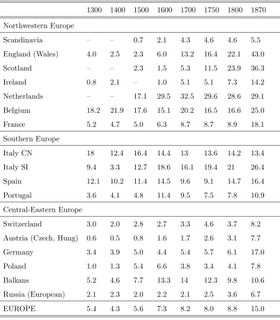
A number of recent studies have pointed to the emergence of northwest Europe as a high wage economy during the early modern period, between the sixteenth and eighteenth cen-turies, with Britain overtaking the Netherlands to become the highest wage economy in Europe (van Zanden, 1999; Allen, 2001; Broadberry and Gupta, 2006), at the same time Britain was among the most urbanized countries in the world, in the …rst half of eighteenth century, at the onset of the industrial revolution (Malanima 2009).
Since one of the key features of the Industrial Revolution was the development of labour saving technology in Britain, it is natural to link the Industrial Revolution to these prior de-velopments in factor prices and the global commercial environment in which they emerged (Broadberry and Gupta, 2009; Allen, 2009). Indeed, a long tradition in economic history links the transition to modern economic growth to the widespread commercialisation of Britain and other parts of northwest Europe between the late medieval period and the Industrial Revolution (Toynbee, 1890; Polanyi, 1944; Britnell and Campbell, 1995). How-ever the precise nature of the links between the Commercial Revolution and the Industrial Revolution has remained unclear.
The de…nition of commercialization used in this paper means more than simply an in-crease in the proportion of output passing through the market (Britnell and Campbell, 1995: 1). Commercial development is characterized by a dramatic change in the informational structure among economic agents –as already emphasized in the theoretical literature by Banerjee and Newman (1998). In particular in this paper we are interested in the growing reliance on anonymous, impersonal relations, as against personalised customary relations, in labour markets following the commercial revolution. Our starting point is Greif (1994) who established an endogenous link between anonymous markets, trading relationships and prices taking as given the level of technology. The contribution of our paper is to establish the link between the degree of anonymity in labour markets and both capital accumulation and the evolution of technology, via the e¤ect of relative prices.
has been …red will be hired again in the future (along the lines of Greif (1994)). Our model thus combines elements of e¢ ciency wages, learning-by-doing and endogenous growth (Hicks, 1932; Arrow, 1962; Romer, 1986) and the institutional enforcement of labour market discipline based on Greif (1994). At the same time, our model is able to deliver a simple closed form solution under the assumption of perfect factor substitutability. Nevertheless, we show the key results to be robus to the relaxation of this assumption with the more realistic assumption of imperfect substitutability.
Our analysis shows, …rst, that the growing commercialisation of the late medieval and early modern periods led to higher wages as the greater anonymity of market relations replaced customary relations in the allocation of labour. Note that this “e¢ ciency wage” argument avoids the objection sometimes levelled at the literature on induced innovation that high wages do not re‡ect high labour costs because the labour is also highly productive. E¢ ciency wages imply higher wages in anonymous commercialized factor markets to induce the same e¤ort as achieved in more personalized customary relationships backed up by close supervision. Second, we show that the resulting rise in the wage/cost of capital ratio led to the adoption of a more capital-intensive technology. Third, this led to a faster rate of technological progress through greater learning by doing on the capital intensive production technology.
Viewed from the perspective of Greif (1994), commercialisation can be interpreted as a switch in the “rules of the game”due to institutional or cultural changes, portrayed in Greif by the distinction between Genoese and Maghribi traders. However, it is worth noting that our model is consistent with a more continuous notion of commercialization that entails a more gradual process of uni…cation of distinct markets, perhaps due to decreasing costs of trade, that dilutes the bonds of customary labour market relationships between employers and workers.
modern period is linked to the Industrial Revolution via its e¤ects on factor prices. Section 5 concludes. Proofs are contained in the Appendix.
2
Related literature
The approach taken here draws on ideas which have been used in the literature on the importance of high wages in stimulating the innovations of the Second Industrial Revolu-tion in late nineteenth century America (Rothbarth, 1946; Habakkuk, 1962; David, 1975; Broadberry, 1997).1 Until recently, there has been a reluctance to cast Britain in the role
of a high wage producer at the time of the Industrial Revolution, since the vast literature on the standard of living debate emphasized the slowness of real wages to rise. However, recent work has emphasized international comparisons of the level of real wages and other factor prices, pointing clearly to Britain’s unusual combination of factor prices (Allen, 2001; 2009; Broadberry and Gupta, 2006; 2009). This is important not only in explaining the adoption of modern technology, but also its non-adoption in other countries with di¤erent factor prices, a point emphasized in the theoretical literature by Zeira (1998) and in the historical literature by Broadberry and Gupta (2009), Allen, (2009) and Fremdling (2000). The current paper suggests a link between the two main strands of the macro-development literature: the institutional approach (e.g. North, 1990; Greif, 2004; 2006; Acemoglu and Robinson, 2006) and uni…ed growth theory (e.g. Galor and Weil, 1999; 2000; Galor and Moav, 2000; Hansen and Prescott 2002; Doepke, 2004; Galor, 2005; Cervellati and Sunde, 2005, Madsen, Ang and Banerjee, 2010). The institutional approach emphasizes the im-portance of trade and commercial development, which are supported by an appropriate institutional framework, while uni…ed growth theory links technological progress to wages via an emphasis on human capital, with families choosing to have fewer but more highly educated children as technology becomes more complex. Our approach sees the two the-oretical frameworks as complementary: establishing the right institutional framework to encourage the development of trade leads to higher wages, which then has the e¤ects on technology traced out in uni…ed growth models Of course this does not preclude the op-eration of the Malthusian links between wages and population stressed in uni…ed growth
theory.
Furthermore, within the institutional approach, our paper provides a link between com-mercial development and economic growth that is complementary to the links suggested by Acemoglu et. al. (2005) and by Galor and Mountford (2006). Acemoglu et. al. focus on the impact of Atlantic trade on institutions, with growing trade strengthening the position of merchants in northwest Europe and enabling them to impose e¤ective constraints on the executive, hence less extractive institutions. Galor and Mountford (2006) show that trade might have generated a demographic boom in non industrial countries, specialized in the production of unskilled-labor-intensive goods, hence fostering the process of divergence. Our approach focuses on an alternative link between trade and growth, with increasing commercialisation a¤ecting factor prices, choice of technology and the rate of technological progress.
Our setting is also consistent with the idea that capital was an important engine of growth along the process of development (Galor and Moav 2004), since we emphasize the e¤ect of high wages on the capital intensity of production and the subsequent rate of technological progress. Along similar lines Voigtländer and Voth (2010) emphasize the importance of the e¤ect of growing capital inputs on TFP increases for the …rst phase of industrialization.2
3
The model
In this section, we introduce our concept of anonymity and endogenous technological progress via learning by doing. We show that a higher degree of anonymity, arguably generated by the commercial revolution, made more di¢ cult monitoring workers and led to an increase in wages and subsequently to more capital intensive production. This process eventually led to a technological increase in labour e¢ ciency that we characterize as the industrial revolution.
3.1
Workers
Time periods are indexed by t, t = 0;1;2; :::. There is a mass N of identical risk averse workers. There is a probabilitydthat at each timet, the worker dies or permanently retires from working. Since the number of workers is …xed at each period, there aredN new workers in the economy so that the labor supply is always constant. Workers have an inter temporal discount factor which, for notational simplicity, we multiply by the probability of surviving next period, (1 d); and de…ne the resulting product as <1:
At any period t, each worker can be either employed or unemployed and is endowed with a …xed amount of e¤ort that can be costlessy provided. If she is unemployed she uses her e¤ort in a backyard informal activity, which yields At; where At is a
technolog-ical parameter, linked to the general economic environment at any time t; which we will characterize later; if she is employed she earns a wage wt:
Since e¤ort cannot be observed, employed workers can either shirk or work (i.e. choose an e¤ort level e 2 f0;1g). An employed shirking worker uses her e¤ort for the backyard activity earning At in addition to the wage o¤ered by the employer. She can be detected
with probability 1 p and …red. In this case, a shirking worker who has been …red can look for a job in the next period by "hiding" among the pool of new workers dN and her probability of …nding a new job is q , where (i) q (which is endogenous and will be determined later) is the probability, common to all individuals in the unemployment pool, of being hired and (ii) 2 (0;1) is a parameter, the probability of being detected by a new employer as having shirked in the past and accounts for the level of anonymity in the economy and is known by both workers and employers.
We interpret as the probability that the news that a worker has shirked in the past when employed reached a new employer. We assume that employers are committed, perhaps by customary rules, not to hire the workers if they can observe the signal, and this behavior is common knowledge among all workers.
The parameter measures the degree of anonymity in labour markets and we interpret as an index of commercialization of the economy, and consider a increase of as growing commercialization.3
A non-shirking worker will work in the …rm until termination (which happens with probability d at each t). We note that p+ (1 p) q is the probability that a shirking worker at time t; will still be alive at time t+ 1. We de…ne VE
t (e) as the intertemporal
utility of an employed worker that exercises e¤ort e 2 f0;1g at timet:
We will now write down the conditions required to ensure that at the prevailing wages at time period t, choosing high e¤ort e = 1 is optimal for each employed worker. To this end, by the one-shot deviation principle (Blackwell (1965)), it is su¢ cient to show that no employed worker can gain by deviating and choosing low e¤ort e= 0 for one period at any
t.
Fix a sequence of market wages fwt :t 0g.
The intertemporal utility for an employed non shirking worker is
VtE(1) =wt+ VtE+1(1); (1)
and we have the following expected discounted utilities for an employed worker who shirks once but does not shirk again in the future:
VtE(0) =wt+ At+ ((p+ (1 p) q)VtE+1(1) + (1 (p+ (1 p) q))V
U S
t+1); (2)
where VU S
t is the intertemporal utility of an unemployed worker who has shirked at least
once in the past but does not shirk again if employed in the future i.e.
VtU S = At+ (q VtE+1(1) + (1 q )V
U S
t+1): (3)
Therefore, given the sequence of market wages, the no shirking constraint is met when-ever:
VtE(1) VtE(0): (4)
We assume that at eacht, each worker correctly anticipates future levels ofVtE(e); e2 f0;1g
and VtU S.
3.2
Production and …rms
There is a …xed mass of one identical …rms, indexed by i. We will assume that each …rm has an increasing, strictly concave production function with Harrod-neutral (or labour augmenting) technological progressF(k; Atl).
To begin with, we assume perfect substitution between factors:
F(k; Atl) = ( k+ (1 )Atl) ; <1 (5)
We will return to the general case (allowing for imperfect substitutability between the factors of production) in the next subsection.
We assume that At evolves over time according to
At= (1 )At 1+ a(Kt 1), 0< <1: (6)
The interpretation is that the prevailing technology in any periodtis a weighted average of the technology prevailing in the preceding period and any new knowledge created in that period. We assume that the new knowledge created in the preceding period is an increasing function of the aggregate capital stock Kt 1 att 1. This assumption can be interpreted
as productivity growth through learning by doing (e.g. Arrow (1962) and Romer (1986)), speci…cally the stock of knowledge increases with the amount of capital used within each …rm i.e. a(0) = 0and a0(K
t 1)>0.
Firms borrow capital from an external capital market at an exogenously given interest rate r; the capital supply is perfectly elastic and, in equilibrium, make non-zero pro…ts, given the assumption <1, which implies decreasing return to scale on capital and labor factors. Therefore, pro…ts of the …rm can be interpreted as a return to a …xed factor of production namely entrepreneurship.
All …rms are price-takers. At each t, each …rm i takes the interest rate r and the technological parameter At as given. Although …rms’ choices at time t 1 in‡uence the
time period. Therefore, at each t, each …rm maximizes current period pro…ts only i.e.
max
wi;t;ki;t;li;tF(k; Atl) wi;tli;t rki;t (7)
3.3
Market equilibria and steady state
We de…ne a market equilibrium for a …xed as follows:
A market equilibrium is a sequence of (Kt; Lt; wt; At :t 1)such that at each t = 0;1: : ::
1. Given r and At, for each …rms wi;t =wt li;t =Lt; ki;t =Kt maximizes pro…ts,
2. No employed worker shirks i.e. wt satis…es the no shirking constraint(4),
3. At =At 1+a(Kt 1).
At a steady state Kt = Kt+1 = K , Lt = Lt+1 = L and At = At+1 = A for all t.
From (6), it follows thatA =a(K ). Therefore, the steady state (long-run) values of the variables at a market equilibrium are denoted by(K ; L ; w ; A =a(K )).
Next, we characterize the market equilibrium in our model …rst for the case of perfect substitutes and then for the general case with imperfect substitutes.
3.4
Market equilibrium with perfect substitutes
Consider, …rst, the pro…t maximizing problem for each …rm (7) with
F(k; Atl) = ( k+ (1 )Atl) ; <1:
First, note that in equilibrium, for each …rm, at each t, at an interior solution the …rst order conditions with respect to capital and labour ki;t and li;t are:
(1 )At ( ki;t+ (1 )Atli;t) 1 = wt (8)
( ki;t+ (1 )Atli;t) 1 = r (9)
we can rewrite (8) as:
ki;t =
(1 )Atli;t + r
1 1
and substituting it in (9) we obtain simply
wt =At
1
r (11)
i.e. at each t, at an interior solution, the factor price ratio wtr is equal to the constant (factors of production are perfect substitutes) slope of the isoquantAt 1 .
Let ! = 1 r, so that wt = !At or equivalently, ! = wt
At. We interpret ! as wages
measured in e¢ ciency units of labour. In the case with perfect substitutes, as we shall see below,! will remain constant over time but asAt will evolve over time, real wageswt will change over time.
Withwt =!At, we can decompose the value functions (1), (2) and (3) for each worker
as follows:
VtE(1) = AtvEt (1) (12) VtE(0) = AtvEt (0) (13)
VtU S = AtvU St : (14)
wherevE
t (e)andvtU Sdepend on!. Furthermore, we note that in equilibrium the no shirking
constraint (4) must bind, therefore
vEt (1) =vtE(0): (15) It follows that solving recursively the system given by expressions (14), (13) and (12) for the steady state values of vE
t (1); vtE(0) and vtU S and using the equilibrium condition
(15), we have
! = (1 p(1 q ))
(1 (p+ (1 p)q )): (16)
employed workers, therefore the equation qdN =dL must hold. Let us then de…ne
q=q(L) = L
N; (17)
Using (16) and (17), we can then rewrite the no shirking constraint as
!(L; ) = (1 p(1 q(L) ))
(1 (p+ (1 p)q(L) ): (18)
from which we note that, di¤erently from the classical model with "e¢ ciency wages", our equilibria are compatible with no unemployment N = L i.e. it is possible that when
q(L) = 1; w <1 for low values of i.e. when the degree of anonymity in the market isn’t too high.
Moreover,
lim
L!0!(L; ) =
(1 p) (1 p) !:
independent of the value for . Therefore, as long as
(1 p) (1 p) <
1
r; (19)
there is a positive level of steady state employment L for each value of . Further, as
(1 p(1 q(L) )) is increasing in both L and and (1 (p + (1 p)q(L) )) is decreasing in bothL and so that the ratio (1 ((1 p+(1p(1 pq)(qL() ))L) )) is increasing in both L and
, an increase in the value of must lower employment i.e. decrease L. We depict the impact of a changing value of in Figure 1 below.
Figure 1 shows how (11) and (18) determine the equilibrium labor demand. The Non Shirking area is above the upward bending lines, AS and AS’, determined by equation (18). For higher level of (i.e. higher market anonymity), the line rotates upward, going from AS to AS’. The straight line is the equilibrium wage, characterized by (11). At the equilibrium, the higher degree of anonymity 0 corresponds to a lower level of employment
L0, as we can see in the …gure comparing equilibriumE0 with equilibriumE.
N O
E E’
ω
ω
L’ L
ω
σ
'
σ
S’ S
[image:14.595.172.448.139.346.2]A
Figure 1: Labor market with pefect substititute production factors
of unemployment wages can go down so that …rms can reemploy workers until the new level of unemployment is reached at a wage not higher than before. Therefore, with perfect substitutability, the only labor market e¤ect of an increase in the degree of anonymity is a lowering of the level of employment. In the following section, where we relax the assumption of perfect substitutability, we show that the labor market will be also cleared by an increase in equilibrium wages. We will now analyze the e¤ect of anonymity on capital allocation, which will have an impact on productivity in the long-run. Note also that although the wage in e¢ ciency units ! remains constant, real wages wt will evolve over time as At
changes over time.
Note from (18) that the equilibrium employment L is not dependent on At and Kt;so
that we will write equilibrium employment as a function of the degree of anonymity alone i.e. L( ), with L0( )<0. Using the demand for capital of a single …rm, (10) and recalling
that in equilibrium all …rms are equal, so that Kt =ki;t and L( ) = li;t for all …rms i at
eacht, aggregate capital at each timet is determined by the following equation:
Kt =
(1 )
AtL( ) +
1 r 1 1
Taken together with (6), (20) determines the evolution of capital and technology over time. The following proposition characterizes the dynamics for the case where capital and labour are perfect substitutes:
Proposition 1 Under condition (19), the relationship between anonymity, technology and
capital in the long-run, when capital and labour are perfect substitutes, is given by the
following:
(i)For each , there is a unique steady state with a positive capital stock K =K( ),
a positive level of employment L =L( ), and technology A =a(K( ))>0;
(ii) The steady state capital stock K( ), technology A = a(K( )) and real wages
w =!a(K( )) are all increasing in the degree of anonymity .
(iii) The steady state is locally a saddle and further, whenever a0(K ) <
(1 )L( ) the
steady state is locally stable.
Proof: See the appendix
The above proposition shows that there is a unique positive steady state value of the capital stock K corresponding to each value of . If the degree of anonymity increases to 0 > , what are the short-run and long-run e¤ects? With k and l perfect substitutes, wages in e¢ ciency units have to be constant and therefore, the labour market clears after a change in through a reduction in employment. In turn, a reduction in employment increases the demand for capital and therefore, results in a bigger capital stock, increased real wages and a higher level of technology in the long run. Further, as employment levels for a …xed do not depend on the current capital stock, if technology is not too sensitive to small change in capital stock, the steady state is locally stable.
In the following section, we relax the assumption of capital and labor being perfect substitutes and show that the main results will not change. The main di¤erence is that, after an increase in ; the labor market will perhaps more realistically clear through an increase of wages in e¢ ciency unit, !:
3.5
Market equilibrium with imperfect substitutes
paper, we generalize the dynamics to the case where the factors of production are imperfect substitutes.
We will assume that the production function F(k; Al) is increasing in both its argu-ments, is strictly concave and smooth in k and l; that Fkl00(k; Al) < 0 (i .e. the factors of production are (imperfect) substitutes), and limk!0Fk= liml!0Fl =14.
At each t, in equilibrium, the …rst order conditions characterizing pro…t maximizing input choices are:
Fk(kt; Atlt) = r (21)
AtFl(kt; Atlt) = wt: (22)
Assume that at each t, wt = !tAt i.e. the market wage is linear in At so that, as
before, we can decompose the value functions for each worker with VtE(1) = AtvEt (1), VE
t =AtvtE(0)andVtU =AtvtU wherevtE(1),vEt (1)andvUt depend on!t. The interpretation
of !t = wAtt is the same as before (i.e. real wage expressed in e¢ ciency units). Recalling
that in equilibrium all …rms are equal, so that Kt=ki;t and Lt=li;t for all …rms iat each t, we can determine the aggregate equations describing the steady state (where we have used (6)) as follows:
Fk(K ; A(K )L ) = r (23)
Fl(K ; A(K )L ) = !t: (24)
with the no shirking constraint (4)
! =!(L ; ) = (1 p(1 q(L ) ))
(1 (p+ (1 p)q(L ) )): (25)
where q(L ) = L N.
What is the impact of a change in the degree of anonymity on the steady state values of capital stock, employment and wages?
By examining the impact of a higher degree of anonymity on the steady state capital
4An example of a production function that satis…es all these assumptions is F(k; Al) = ( k + (1 ) (Atl) )
1
labour ratio and wages, the following proposition generalizes Proposition 1 to the case where capital and labour are imperfect substitutes in production:
Proposition 2 Suppose that the production function is concave and satis…es the
assump-tion that capital and labour are imperfect substitutes i..e. F00
kl(k; Al)<0. The relationship
between anonymity, technological and the equilibrium capital dynamics when capital and
labour are imperfect substitutes is given by the following:
(i) For each >0, there is a unique steady state with positive capital stock K =K( )
and employment level L =L( );
(ii) The steady state stock capital labour ratio KL = KL( )( ), technology A = a(K( ))
and real wages w =!(L( ))a(K( )) are all increasing in the degree of anonymity ;
(iii) Assume that in the vicinity of the steady state, at each t, agents expect that future
employment and wage levels will be the same as current employment levels. For each >0,
the steady state is locally a saddle. Further, there exists 0 < < 1 such that whenever
< <1 the steady state is locally stable.
Proof: See the appendix.
The above proposition shows that there is a unique positive steady state value of the capital stock K corresponding to each value of . If the degree of anonymity increases to
0 > , what are the short-run and long-run e¤ects?
Note that in the previous section, with k and l perfect substitutes, wages in e¢ ciency units have to be constant and therefore, the labour market clears after a change in through a change in employment. Starting from the steady state capital stock and employment corresponding to , with imperfect substitutes in the model, a change in results in a change in (real) wages in the short-term i.e. in a change in !t (as always At is …xed at t
and will change from periodt+ 1). In response to an increase in!t, no …rm will substitute
labor with capital entirely given that the marginal productivity of capital will decrease, and the marginal productivity of labour will increase, as more capital is employed. Therefore, when capital and labour are imperfect substitutes in production, wages in e¢ ciency units are no longer held constant and both wages in e¢ ciency units and employment will adjust to clear the labor market.
progress (driven by learning by doing), the steady state capital and real wages associated with a higher level of anonymity (and hence, technology) is also an increasing function of
.
In order to examine the local stability of the steady state, we assume that in the vicinity of the steady state, at eacht, agents expect that future employment and wage levels will be the same as current employment levels. Under this assumption, when workers are patient enough, current wages in e¢ ciency units aren’t too sensitive to small changes in current labour market conditions. Therefore, small changes in current labour market conditions do not result in large changes in relative factor prices and therefore, capital stock and technology. Therefore, when workers are patient enough, the steady state is locally stable.
4
Historical evidence: the transition to modern
eco-nomic growth in Northwest Europe, 1300-1850
We now examine the transition to modern economic growth, combining historical evidence with the theoretical model presented in the previous section. We argue that the Commercial Revolution of the early modern period was an important staging post on the road to the Industrial Revolution because of the e¤ects of growing commercialisation on factor prices. Increasing anonymity due to growing commercialisation led to an increase in the price of labour relative to the price of capital, which induced a substitution into a more capital intensive technology and an acceleration of technological progress through learning by doing. We argue further that the fact that commercialisation went further in Britain than in the rest of Europe helps to explain why the Industrial Revolution occurred …rst in Britain.
4.1
Growing commercialisation
in north Italy and in the Low Countries. While urbanization stalled in north Italy after 1500, there was a brief surge in Portugal and to a lesser extent Spain during the sixteenth century, following the opening up of the new trade routes to Asia and the New World. However, the most dramatic growth of urbanization in the early modern period occurred in the Netherlands in the sixteenth and seventeenth centuries and in England during the seventeenth and eighteenth centuries as those countries displaced the Iberian powers in long distance trade and commercialized their domestic economies to an unprecedented extent.
This growth of commercialisation had implications for the degree of anonymity in eco-nomic relations, in factor markets as well as in product markets and this, in turn, had implications for wages. When workers were employed in small-scale enterprise in rural lo-cations where they formed part of a close-knit community, the problem of securing e¤ort from workers could be solved through reliance on customary relations backed up by close supervision. As people moved to towns where they were unknown to their neighbors and potential employers, it became necessary for employers to …nd new ways to elicit e¤ort. In the model above, this is captured by a change in , the degree of anonymity in the economy, which lies at the heart of the no-shirking constraint equations (18) and (25).
One approach to dealing with this increase in the degree of anonymity in market based relationships, which was widely adopted in large urban enterprises during the early stages of the Industrial Revolution, was payment by results or piece rates (Pollard, 1965: 189-191). Of course, piece rates had also been used in a rural setting during the early modern period as part of the putting out system, but their “discovery”in the context of urban industry in the eighteenth century was often greeted as “an innovation of major signi…cance”(Pollard, 1965: 190). However, as Huberman (1996: 17-32) points out, attempts to manage the wage-e¤ort bargain through piece rate payments in early nineteenth century Lancashire often met with little success unless accompanied by the payment of an e¢ ciency wage above the spot-market rate. Rather than risk the prospect of losing a job with a wage above the spot market rate, a worker employed at the e¢ ciency wage is deterred from shirking (Shapiro and Stiglitz, 1984).5
4.2
Changing factor prices
Table 2 sets out the pattern of silver wages in Europe. The silver wage is the silver content of the money wage in the local currency, and is useful for comparing wages across countries on a silver standard. Note …rst that Northwestern Europe saw substantial silver wage growth in the century after the Black Death of the mid-fourteenth century and again during the early modern period after 1500, as well as during the Industrial Revolution period from the mid-eighteenth century, when Britain …nally overtook the Netherlands decisively. Second, note that although southern Europe shared in the rise in the silver wage following the Black Death, from the mid …fteenth century the region was characterized more by ‡uctuations than by trend growth in the silver wage. Third, central and eastern Europe were also characterized more by ‡uctuations than by trend growth in the silver wage from the mid-fourteenth century. This is the pattern that would be expected from the conventional economic history of Europe, with the Mediterranean region playing the leading economic role during the …rst half of the millennium, but with northwest Europe forging ahead after 1500.
We have focused so far on wage di¤erences within Europe, but a complete picture of the transition to modern economic growth also requires a consideration of wage di¤erences between Europe and Asia. Broadberry and Gupta (2006) provide some evidence of this Great Divergence in the form of silver wage di¤erences, shown here in Table 3. Silver wages in India and the Yangzi delta region of China were already lower than those in England by the beginning of the seventeenth century, and then fell further behind. Contrary to the revisionist claims of Pomeranz (2000), Parthasarathi (1998) and Frank (1998) that the richest parts of Asia remained at the same level of development as the richest parts of Europe until as late as 1800, they appear closer to the poorer parts of Europe.
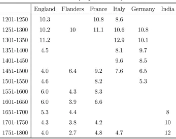
We are interested in the incentives to adopt capital intensive technology. Hence we need also to examine the cost of capital, an important element of which is the rate of interest. Nominal interest rates for a number of countries are presented in Table 4. Note that since interest rates changed together across Europe, it is reasonable to assume them exogenous with respect to each single European economy, so that intra-European di¤erences in the factor price ratio were driven by wage rate changes, as highlighted in our model. Table
4 suggests a rate of interest in Europe around 10% in the late medieval period, falling to 5-6% in the aftermath of the Black Death, 1350-1400. There was a further reduction in European rates of interest during the …rst half of the eighteenth century, to around 3-4%. By this point, interest rates were substantially lower in Europe than in other parts of the world such as India, where rates remained at medieval levels. Growing commercialisation was thus accompanied by declining interest rates. The downward trend of interest rates in Europe, combined with the increase in wages, translates into an increase in the wage/cost of capital ratio, raising the incentives to substitute capital for labour in production. The greater increase of wage rates in northwest Europe meant that the incentive to adopt capital intensive production methods was also greater in that region.
4.3
Factor prices and technology
Recent work by Broadberry and Gupta (2006; 2009) and by Allen (2009) emphasize the important role of factor prices in explaining the key technological choices of the Industrial Revolution period. Broadberry and Gupta (2009) analyze the shift of competitive advan-tage in cotton textiles between India and Britain. India was the world’s major producer and exporter of cotton textiles during the early modern period, but was displaced from this position by Britain during the Industrial Revolution. Broadberry and Gupta (2009) point to the much higher wages in Britain than in India already in the late seventeenth century, when Indian cotton textiles were imported into Britain by the East India Company. This can be seen in the …rst column of Table 5. Combined with the smaller di¤erences in the cost of raw cotton and the cost of capital, this presented British producers with a severe total factor input (TFI) price disadvantage. To get to a point where the free on board price was cheaper in Britain, required a shift to more capital intensive technology and a sustained period of technological progress to increase total factor productivity (TFP). For much of the eighteenth century, the ‡edgling British cotton industry required protection, although the point at which the shift in competitive advantage from India to Britain occurred varied by type of yarn or cloth (as a result of di¤erent input costs) and by market (as a result of transport costs).
the period 1770-1820. This would be quite consistent with the 1.9 per cent per annum TFP growth rate estimated by Harley (1993: 200) for the British cotton industry between 1780 and 1860, together with slowly rising or stagnating productivity in India. This acceleration of TFP growth following the shift to capital intensive technology can be explained by the greater potential for learning on capital intensive technology.
4.4
Real economic development
In Table 2, we examined the path of silver wages. However, an analysis of the transition to modern economic growth would not be complete without considering the path of real con-sumption wages and GDP per capita. The real concon-sumption wage is obtained by dividing the silver wage with the silver price of basic consumption goods. Real consumption wages of European unskilled building labourers for the period 1300-1850 are shown in Table 6, taking London in the period 1500-49 as the numeraire. The …rst point to note is that real wages followed a similar pattern across the Black Death in the whole of Europe. Complete time series exist for comparatively few cities before 1500, but there is also scattered evidence for other cities. Taken together, the evidence supports the idea of a substantial rise in the real wage across the whole continent of Europe following the Black Death, which struck in the middle of the fourteenth century, wiping out between a third and a half of the popula-tion, when successive waves of the plague are cumulated (Herlihy, 1997). This episode of European economic history is thus broadly consistent with the Malthusian model, with a strong negative relationship between real wages and population (Postan, 1972: 27-40). In the …rst half of the …fteenth century, the real wage was quite uniform across the countries for which we have data, at about twice its pre-Black Death level. From the second half of the …fteenth century, however, Britain and Holland followed a very di¤erent path from the rest of Europe, maintaining real wages at the post-Black Death level and avoiding the collapse of real wages which occurred on the rest of the continent as population growth returned. Considering that in the same period Britain and Holland witnessed an increase in the level of urbanization, as noted above, we can argue that the anonymity is a candidate to explain this emergence of high wages in northwest Europe.
de-veloped Mediterranean Europe from the late sixteenth century. The national income data thus reinforce the conclusion from the silver wage and real wage data and from urbanization rates that Britain and Holland followed a di¤erent path from Italy and Spain. The Indian data con…rm the conventional view that the Great Divergence was already underway during the early modern period, as Europe embarked upon a period of growing commercialisation which would ultimately end up with the Industrial Revolution and the transition to modern economic growth.
4.5
A simple econometric test
Our hypothesis is that commercialization led to high wages throughout Europe, in the short-run through the e¢ ciency wage channel (increasing !t), and in the longer term
be-cause of the improved technology At. So far we have reviewed evidence showing that the
urbanization–that we consider as a proxy for commercialization–, wage rate and GDP per capita data are related in a way which is at least consistent with the direction of causal-ity proposed in the model. In what follows, we will estimate a simple econometric model linking real wages and urbanization.
There are at least two main problems in establishing causality from urbanization to wages: (i) a possible omitted variable bias since wages and urbanization can both be a by-product of underlying economic trends e.g. cycles or technological improvements, or other shocks; (ii) a possible problem of endogeneity., given that urbanization can be the e¤ect rather than the cause of higher wages.
Given the constraints of available data, we will address (i) by controlling for country GDP and introducing the year …xed e¤ect in the regressors, and (ii) by instrumenting urbanization at time t, with urbanization 50 years before.
Therefore, we estimate the following equation:
wagei;t =ci+ gdpi;t:+ urbanizationi;t +yeart+"i;t; (26)
where index i indicates the city, and t indexes time.
Data on wages are aggregated at city level and are taken from table 2, while data on
the idiosyncratic economic cycles and technology, the years dummies yeart control for the
e¤ects generated by common shocks. Dummy variable ci controls for city …xed e¤ects.
Table 8 displays the results of the estimations. Column 1 shows the above described pattern between wages and urbanization, column 2 shows that this relation is still signi…cant when we control for the aggregate shocks by introducing the year e¤ect. In column 3 we introduce country GDP to control for some country level omitted variable. In column 4 we use a two stage least squares estimator by using urbanizationt 1 (therefore 50 years
before) as an instrument forurbanizationt:Finally in column 5 we introduce the wages at
time t 1 in the 2SLS estimation to control for the e¤ect of wages’serial correlations. In all speci…cations and consistently with our model, the coe¢ cient of urbanization is positive and highly signi…cant.
5
Concluding comments
We have argued that commercialisation played a pivotal role in the transition to modern economic growth. We see the growing commercialisation of the late medieval and early modern periods as leading to the acceleration of technological progress during the Industrial Revolution period via its e¤ects on factor prices. The argument can be summarized as follows: (1) Commercialisation raised wages as a growing reliance on impersonal labour market relations in place of customary relations with a high degree of monitoring led to the adoption of e¢ ciency wages. (2) The resulting rise in the wage/cost of capital ratio led to the adoption of a more capital-intensive production technology. (3) This led to a faster rate of technological progress through greater learning by doing on the capital intensive technology.
References
[1] Acemoglu, D. (2009) When Does Labor Scarcity Encourage Innovation? NBER Work-ing Paper No. 14809
[3] Acemoglu, D., Johnson, S. and J.A. Robinson, (2005), “The Rise of Europe: Atlantic Trade, Institutional Change and Economic Growth”, American Economic Review, 95: 546-579.
[4] Allen, R.C. (2001), “The Great Divergence in European Wages and Prices from the Middle Ages to the First World War”, Explorations in Economic History, 38, 411-447.
[5] Allen, R.C. (2009), The British Industrial Revolution in Global Perspective, Cam-bridge: Cambridge University Press.
[6] Álvarez-Nogal, C. and Prados de la Escosura, L. (2009), “The Rise and Fall of Spain, 800-1850”, Universidad Carlos III, Madrid.
[7] Arrow, K.J. (1962), “The Economic Implications of Learning by Doing”, Review of Economic Studies, 29, 155-173.
[8] Banerjee A.V., and A.F. Newman (1998). “Information, the Dual Economy, and De-velopment,” Review of Economic Studies 64, 631-653.
[9] Blackwell, D. (1965), “Discounted Dynamic Programming,” Annals of Mathematical Statistics 36, 226–235.
[10] Álvarez-Nogal, C. and Prados de la Escosura, L. (2009), “The Rise and Fall of Spain, 800-1850”, Universidad Carlos III, Madrid.
[11] Britnell, R.H. and Campbell, B.M.S. (eds.), (1995), A Commercialising Economy: England 1086 to c.1300, Manchester: Manchester University Press.
[12] Broadberry, S.N. (1997), The Productivity Race: British Manufacturing in Interna-tional Perspective, 1850-1990, Cambridge: Cambridge University Press.
[13] Broadberry, S.N., Campbell, B., Klein, A, Overton, M. and B. van Leeuwen, (2011), “British Economic Growth, 1270-1870”, London School of Economics.
[14] Broadberry, S.N. and B. Gupta, (2006), “The Early Modern Great Divergence: Wages, Prices and Economic Development in Europe and Asia, 1500-1800”, Economic History Review, 59, 2-31.
[16] Broadberry, S.N. and B. Gupta, (2011), “India and the great Divergence: An Anglo-Indian Comparison of GDP per capita, 1600-1871”, London School of Economics and University of Warwick.
[17] Buyst, E. (2009), Estimates of Economic Growth in the Southern Low Coun-tries/Belgium, c.1770-1846”, Centre for Economic Studies, Katholieke Universiteit Leuven.
[18] Cervellati, M. and U. Sunde, (2005),. “Human capital formation, life expectancy, and the process of development”. American Economic Review, 95(5), 1653-1672. [19] Clark, G. (1988), “The Cost of Capital and medieval Agricultural technique”,
Explo-rations in Economic History, 25, 265-294.
[20] David, P.A. (1975), Technical Choice, Innovation and Economic Growth, Cambridge: Cambridge University Press.
[21] Doepke, Matthias, (2004), Accounting for Fertility Decline During the Transition to Growth, Journal of Economic Growth, 9(3):347-383.
[22] Frank, A.G. (1998), ReOrient: The Silver Age in Asia and the World Economy, Berke-ley: University of California Press.
[23] Fremdling, R. (2000), “Transfer Patterns of British Technology to the Continent: The Case of the Iron Industry”, European Review of Economic History, 4, 195-222. [24] Galor, O. (2005). From stagnation to growth: Uni…ed growth theory. In: P. Aghion
and S. Durlauf (eds), Handbook of economic growth, Vol. 1A. Amsterdam: North-Holland.
[25] Galor, O., Moav, O. (2000). “Ability biased technological transition, wage inequality and growth ·”, Quarterly Journal of Economics 115, 469-498.
[26] Galor, O., and Moav, O. (2004). "From physical to human capital accumulation: In-equality and the process of development". Review of Economic Studies, 71, 1001-1026.
[28] Galor, O. and A. Mountford (2006). “Trade and the Great Divergence: The Family connection”, American Economic Review 96, 299-303.
[29] Galor, Oded and David Weil, (1999),."From Malthusian Stagnation to Modern Growth", American Economic Review Papers and Proceedings, 89(2):150-154. [30] Galor, O., and Weil, D. (2000). "Population, technology and growth: From the
malthu-sian regime to the demographic transition and beyond". American Economic Re-view, 90, 806-828.
[31] Greif, A. (1994), “Cultural Beliefs and the Organization of Society: A Historical and Theoretical Re‡ection on Collectivist and Individualist Societies”, Journal of Po-litical Economy, 102, 912-950.
[32] Greif, A. (2006) "Institutions and the Path to the Modern Economy, Lessons from Medieval Trade". New York, Cambridge University Press.
[33] Habakkuk, H.J. (1962), American and British Technology in the Nineteenth Century, Cambridge: Cambridge University Press.
[34] Hansen,G.D.,and Prescott, E. (2002). "Malthus to solow. American Economic Re-view", 92(4), 1205-1217.
[35] Harley, C.K. (1993), “Reassessing the Industrial Revolution: A Macro View”, in Mokyr, J. (ed.), The British Industrial Revolution: An Economic Perspective, Boulder, Colorado: Westview, 171-226.
[36] Herlihy, D. (1997), The Black Death and the Transformation of the West, Cambridge, MA: Harvard University Press.
[37] Hicks, J.R. (1932), The Theory of Wages, London: Macmillan.
[38] Huberman, M. (1996), Escape from the Market: Negotiating Work in Lancashire, Cambridge: Cambridge University Press.
[39] Maddison, A. (2003), The World Economy: Historical Statistics, Paris: Organisation for Economic Co-operation and Development.
[41] Malanima, P. (2009), PreModern European Economy: One Thousand Years (10th -19th Centuries, Leiden: Brill.
[42] Malanima, P. (2011), “The Long Decline of a Leading Economy: GDP in Central and Northern Italy, 1300-1913”, European Review of Economic History, (forthcoming). [43] Moosvi, S. (2001), “The Indian Experience 1600-1900: A Quantitative Study”, in Panikkar, K.N., Byres, T.J. and Patnaik, U. (eds.), The Making of History: Essays Presented to Irfan Habib, New Delhi: Tulika, 328-358.
[44] North, D.C. (1990), Institutions, Institutional Change and Economic Performance, Cambridge: Cambridge University Press
[45] Pamuk, S. (2007), “The Black Death and the Origins of the ‘Great Divergence’across Europe, 1300-1600”, European Review of Economic History, 11, 289-317.
[46] Parthasarathi, P. (1998), “Rethinking Wages and Competitiveness in the Eighteenth Century: Britain and South India”, Past and Present, 158, 79-109.
[47] P…ster, U. (2009), “German Economic Growth, 1500-1850”, Historisches Seminar, Westfälische Wilhelms-Universität Münster.
[48] Polanyi, K. [1944] (1957), The Great Transformation, London: Bacon Hill.
[49] Pollard, S. (1965), The Genesis of Modern Management: A Study of the Industrial Revolution in Great Britain, London: Arnold.
[50] Pomeranz, K. (2000), The Great Divergence: China, Europe, and the Making of the Modern World Economy, Princeton, NJ: Princeton University Press.
[51] Postan, M. (1972), The Medieval Economy and Society: An Economic History of Britain in the Middle Ages, London: Weidenfeld and Nicolson.
[52] Romer, Paul M. (1986): “Increasing Returns and long-run Growth,”Journal of Polit-ical Economy, 94, 1002–37.
[53] Rothbarth, E. (1946), “Causes of the Superior E¢ ciency of USA Industry as Compared with British Industry”, Economic Journal, 56, 383-390.
[54] Shapiro, C. and Stiglitz, J.E. (1984), “Equilibrium Unemployment as a Worker Disci-pline Device”, American Economic Review, 74, 433-444.
[56] van Zanden, J.L. (1999), “Wages and the Standard of Living in Europe, 1500-1800”, European Review of Economic History, 3, 175-97.
[57] van Zanden, J.L. and van Leeuwen, B. (2011), “The Origins of ‘Modern Economic Growth’? Holland between 1347 and 1807”, Utrecht University.
[58] Voigtländer, N. and Voth, H.-J. (2010), “How the West ‘Invented’ Fertility Restric-tion”, UPF Barcelona.
[59] Vollrtah, D, (2011) "The Agricultural Basis of Comparative Development," Journal of Economic Growth, 16(4), pp. 343-370
TABLE 1: European urbanization rates (%)
1300 1400 1500 1600 1700 1750 1800 1870 Northwestern Europe
Scandinavia – – 0.7 2.1 4.3 4.6 4.6 5.5 England (Wales) 4.0 2.5 2.3 6.0 13.2 16.4 22.1 43.0 Scotland – – 2.3 1.5 5.3 11.5 23.9 36.3 Ireland 0.8 2.1 – 1.0 5.1 5.1 7.3 14.2 Netherlands – – 17.1 29.5 32.5 29.6 28.6 29.1 Belgium 18.2 21.9 17.6 15.1 20.2 16.5 16.6 25.0 France 5.2 4.7 5.0 6.3 8.7 8.7 8.9 18.1 Southern Europe
Italy CN 18 12.4 16.4 14.4 13 13.6 14.2 13.4 Italy SI 9.4 3.3 12.7 18.6 16.1 19.4 21 26.4 Spain 12.1 10.2 11.4 14.5 9.6 9.1 14.7 16.4 Portugal 3.6 4.1 4.8 11.4 9.5 7.5 7.8 10.9 Central-Eastern Europe
Switzerland 3.0 2.0 2.8 2.7 3.3 4.6 3.7 8.2 Austria (Czech, Hung) 0.6 0.5 0.8 1.6 1.7 2.6 3.1 7.7 Germany 3.4 3.9 5.0 4.4 5.4 5.7 6.1 17.0 Poland 1.0 1.3 5.4 6.6 3.8 3.4 4.1 7.8 Balkans 5.2 4.6 7.7 13.3 14 12.3 9.8 10.6 Russia (European) 2.1 2.3 2.0 2.2 2.1 2.5 3.6 6.7 EUROPE 5.4 4.3 5.6 7.3 8.2 8.0 8.8 15.0 Source: Paolo Malanima (2009).
TABLE 2: Daily silver wages of European unskilled building laborers
(grams of silver per day)
1300 1350 1400 1450 1500 1550 1600 1650 1700 1750 1800
Northwestern Europe
London 2.9 3.4 4.5 3.8 3.2 4.6 7.1 9.7 10.5 11.5 17.7 Amsterdam 3.1 4.7 7.2 8.5 8.9 9.2 9.2 Antwerp 3.5 3.1 3.0 5.9 7.6 7.1 6.9 6.9 7.7 Paris 2.8 5.5 6.6 6.9 5.1 5.2 9.9 Southern Europe
Valencia 5.6 5.2 4.2 6.6 8.8 6.9 5.7 5.1 – Madrid – 6.3 8.0 – 5.1 5.3 8.0 Florence/Milan 2.2 4.5 3.8 3.5 2.9 3.8 4.7 4.1 3.2 2.9 3.1 Naples 3.3 3.5 5.3 4.8 4.8 3.8 3.8 Central-Eastern Europe
Gdansk 2.1 2.1 3.8 4.3 3.8 3.7 4.8 Warsaw – 2.5 3.2 2.7 1.9 3.4 4.9 Krakow 2.7 2.1 1.9 2.9 3.4 2.9 2.2 2.9 2.4 Vienna 4.0 3.2 2.7 2.6 4.4 3.5 3.2 3 2.1 Leipzig – 1.9 3.5 3.9 3.7 3.1 4.4 Augsburg 2.1 3.1 4.0 4.7 4.2 4.3 –
Source: Broadberry and Gupta (2006: 7).
TABLE 3: Silver wages of unskilled labourers
(grams of silver per day)
A. Silver wages in England and India
Date England India India/England 1550-99 3.4 0.7 0.21
1600-49 4.1 1.1 0.27 1650-99 5.6 1.4 0.25 1700-49 7.0 1.5 0.21 1750-99 8.3 1.2 0.14 1800-49 14.6 1.8 0.12
B. Silver wages in England and China
Date England China China/England 1550-1649 3.8 1.5 0.39
1750-1849 11.5 1.7 0.15
Source : Broadberry and Gupta (2006)
TABLE 4: Interest rates (% per annum)
England Flanders France Italy Germany India 1201-1250 10.3 10.8 8.6
1251-1300 10.2 10 11.1 10.6 10.8 1301-1350 11.2 12.9 10.1 1351-1400 4.5 8.1 9.7
1401-1450 9.6 8.5
1451-1500 4.0 6.4 9.2 7.6 6.5 1501-1550 4.6 8.2 5.3 1551-1600 6.0 4.3 8.3
1601-1650 6.0 3.9 6.6
1651-1700 5.3 4.4 8
1701-1750 4.3 3.8 4.2 10 1751-1800 4.0 2.7 4.8 4.7 12
[image:32.595.91.439.447.720.2]TABLE 5: Comparative GB/India costs and prices (India =100)
A. Cost
Wage Raw Cotton P Cost of Capital TFI Price W/W* C/C* R/R*
c.1680 400 182 137 206
c.1770 460 320 113 270
c.1790 663 480 106 357
c.1820 517 127 61 150
B. Prices and TFP
TFI price FOB TFP Price P/P* A/A* c.1680 206 200 103 c.1770 270 200 135 c.1790 357 147 243 c.1820 150 53 283
TABLE 6: Daily real consumption wages of European unskilled
building labourers (London 1500-49 = 100)
1300 1350 1400 1450 1500 1550 1600 1650 1700 1750 1800
Northwestern Europe
London 57 75 107 113 100 85 80 96 110 99 98 Amsterdam 97 74 92 98 107 98 79 Antwerp 101 109 98 88 93 88 92 88 82
Paris 62 60 59 60 56 51 65
Southern Europe
Valencia 108 103 79 63 62 53 51 41
Madrid 56 51 58 42
Florence/Milan 44 87 107 77 62 53 57 51 47 35 26
Naples 73 54 69 88 50 33
Central-Eastern Europe
Gdansk 78 50 69 72 73 61 40
Warsaw 75 66 72 45 64 82
Krakow 92 73 67 74 65 67 58 63 40 Vienna 115 101 88 60 61 63 61 50 27
Leipzig 34 35 57 53 44 53
Augsburg 62 50 39 63 55 50
Source: Broadberry and Gupta (2006: 7);
TABLE 7: GDP per capita levels (in 1990 international dollars)
1250 1300 1350 1400 1450 1500 1550 1600 1650 1700 1750 1800 1850 Northwestern Europe
England 737 730 767 1095 1172 1164 1138 1144 1215 1649 1688 2085 3006 Holland 876 1195 1373 1454 1432 2662 2691 2105 2355 2408 1886 Belgium 929 1089 1073 1203 1264 1357 1497
France 727 841 986 1230
Southern Europe
Spain 1249 1249 1388 1145 1160 1160 1294 1219 1175 1145 1190 1249 1487 Italy 1482 1376 1601 1668 1403 1337 1244 1271 1350 1403 1244 1350 Central-Eastern Europe
Germany 1332 894 1130 1068 1162 1140 1428
Poland 462 516 566 636
Austria 707 837 993 1218
India 684 648 630 587 576 560
Source: Netherlands: van Zanden and van Leeuwen (2011); France, Austria, Poland: Maddison (2005),
England: Broadberry et al. (2011).
Italy: Malanima (2011); Belgium: Buyst (2009), Blomme and van der Wee (1994); Germany: P…ster (2009);
Table 8: E¤ect of Urbanization on Wages: Independent Variable is wage in the main europen cities. In columns 4 and 5, urbanization is instrumented by using urbanization 50 years before. (std errors in brackets)
OLS OLS OLS 2SLS 2SLS
(1) 1300-1800 (2) 1300-1800 (3) 1300-1800 (4) 1300-1800 (5) 1300-1800
b/se b/se b/se b/se b/se
Urbanization 0.459*** 0.360*** 0.318*** 0.649*** 0.658***
(0.061) (0.056) (0.073) (0.158) (0.195)
GDP 0.002* 0.005*** 0.004
(0.001) (0.002) (0.004)
Wage[t-1] 0.226
(1.065)
Year e¤ects No Yes Yes Yes Yes
City e¤ects Yes Yes Yes Yes Yes
A
Appendix
A.1
Proof of Proposition 1:
(i) It follows from (6) and (20) that the steady state level of capital stockK must be the solution to the equation
K =f(K) (27)
where f(K) = (1 )a(K)L( ) + 1 r 1
1 . The LHS of (27) is increasing in K while
f0(K) = (1 )
a0(K)L( ) < 0 as a0(K) > 0. Moreover, lim
K!0f(K) = 1 r
1
1 > 0.
Therefore, there exists a unique positive steady state capital stock K and technology
a(K ).
(ii) The steady state capital stock satis…es the equation
K = (1 )a(K )L( ) + 1 r 1 1
By taking the total derivative of the preceding equation with respect toK and we obtain that
dK
d =
(1 )
a(K )L0( )
1 + (1 )a0(K )L( ) >0
as L0( )<0(from (18)) and a0(K )>0(by assumption).
(iii) Examining the local stability of the steady state requires us to linearize the equa-tions (6) and (20) at the steady state to obtain
2 4 1
(1 )
L( )
0 1
3 5
2 4 dKt
dAt
3
5=
2
4 0 0
a0(K ) 1
3 5
2
4 dKt 1
dAt 1
3 5
so that 2
4 dKt dAt 3 5= 2 4 1 (1 )
L( )
0 1
3 5
2
4 0 0
a0(K ) 1
3 5
2
4 dKt 1
dAt 1
3 5
which after further simpli…cation yields
2 4 dKt
dAt 3 5= 2 4 (1 )
L( ) a0(K ) (1 )(1 )
L( )
a0(K)0 1
3 5
2
4 dKt 1
dAt 1
By computation, it is easily checked that the determinant of the matrix on the RHS of the preceding equation is zero so that if 1 and 2 denote the two eigenvalues of the said
matrix,
1 2 = 0;
1+ 2 =
(1 )
L( ) a0(K ) + (1 )
so that the steady state is always a saddle and is a sink if (1 )L( ) a0(K ) + (1 ) <1
or equivalently,a0(K )<
(1 )L( ).
A.2
Proof of Proposition 2:
(i) We …rst show that there is a unique positive steady state capital stock K and that employment level L exists. Note that the steady state is a solution to the equations:
Fk(K; a(K)L) = r;
Fl(K; A(K)L) = !(L; ):
Consider the equation Fk(K; a(K)L) = r. Under the assumption that Fkk < 0, Fll < 0, Fkl <0,a0(K)>0from the equation Fk(K; a(K)L) =r there exists an implicit function g1(L) = K with
g10(L) = a(K)Fkl
Fkk+Fkla0(K) <0
while from the equationFl(K; a(K)L) =!(L; )there exists an implicit functiong2(L) =
K with
g20(L) = a(K)Fll+!l(L; )
Fkk+Fkla0(K)
<0:
Steady state employment L is the solution tog3(L) = g2(L) g1(L) = 0. Aslimk!0Fk =
liml!0Fl = 1, limL!0g3(L) = 1 while limL!1g3(L) = 0 so that there exists L =
L( ) > 0 such that g3(L ) = g2(L ) g1(L ) = 0. Finally, note that K = K( ) =
g2(L ) = g1(L )>0.
(23) and (24) at the steady state is given by the expression
2
4 Fkk+Fkla0(K ) Fkla(K ) Fkl+Flla0(K ) F
lla(K ) !l
3 5 2 4 dK dL 3 5= 2 4 0 ! 3 5d
where ! =! (L ; ). The determinant,D0, of the preceding matrix can be written as
D0 = (Fkk+Fkla0(K ))!l +a(K ) FkkFll (Fkl)2 >0
as F(:) is strictly concave,Fkl<0,a0(K )>0 and !
l >0. Therefore,
2
4 dK
dL
3
5= 1
D0
2
4 Flla(K ) !l Fkla(K ) Fkl+Flla0(K ) F
kk+Fkla0(K )
3 5 2 4 0 ! 3 5d
so that 2
4 dK
dL
3
5= 1
D0
2
4 Fkla(K )!
(Fkk+Fkla0(K ))!
3 5d
and
dK
d =
Fkla(K )! D0 >0
dL
d =
(Fkk+Fkla0(K ))!
D0 <0
as, from (25), ! >0.
(iii) In order to characterize the local stability of the steady state, we need to characterize how real wages wt change in the vicinity of the steady state as equilibrium employmentLt
changes.
Consider the scenario described by (1), (2), (3) and the no shirking constraint (4). As the no shirking constraint (4) holds as an equality in equilibrium, setting vE
t (1) = vtE(0)
and equating the RHS of (1) and (2) we obtain that at each t,
vtE+1(0) =
(1 (p+ (1 p)qt ))
Substituting forvtE+1(0) in (2) we obtain that at eacht
vtU S = (1 p(1 qt )) (1 (p+ (1 p)qt ))
+ vU St+1
which yields that at each t,
vtU S =X
t0 t
t0 t (1 p(1 qt ))
(1 (p+ (1 p)qt ))
and therefore,
vtE(0) =
(1 (p+ (1 p)qt 1 ))
+X
t0 t
t0 t (1 p(1 qt ))
(1 (p+ (1 p)qt )) :
Further, by computation, from (1) we obtain that at eacht,
vtE(1) =
1
X
t0 t t0 t
!t:
Equating vEt (0) and vtE(1) in the vicinity of the steady state and equating the two as required by the no shirking constraint (4) we obtain that at each t,
1
X
t0 t t0 t
!t =
(1 (p+ (1 p)qt 1 ))
+X
t0 t
t0 t (1 p(1 qt0 ))
(1 (p+ (1 p)qt0 )) :
At this point, we will assume that in the vicinity of the steady state, at each t, agents expect that future employment and wage levels will be the same as current employment levels so thatLe
t0 =Ltand!et0 =!tfor allt0 twhere the superscriptedenotes the expected
level of future employment and future wages. In other words, in order to characterize the dynamics in the vicinity of the steady state,we do not assume that agents have rational expectations.
Under this assumption, it follows that we can write at each t,
!t=
(1 )
(1 (p+ (1 p)qt 1 ))
+ (1 p(1 qt )) (1 (p+ (1 p)qt ))
:
so that at each t in the vicinity of the steady state d!t = gldLt 1 +fldLt where f =
(1 p(1 q(L N) ))
(1 (p+(1 p)q(L N) ))
and g = (1 ) (1 (p+(1 p)q(L
N) ))
Taking the above computation into account and noting that at the steady stateA(K ) =
a(K ), examining the local stability of the steady state requires us to linearize the equations (6), (23) and (24) at the steady state to obtain
2 6 6 4
Fkk a(K )Fkl 0
Fkl a(K )Fll fl 0
0 0 1
3 7 7 5 2 6 6 4 dKt dLt dAt 3 7 7 5= 2 6 6 4
0 0 0
0 gl 0
a0(K ) 0 1
3 7 7 5 2 6 6 4
dKt 1
dLt 1
dAt 1
3 7 7 5
where Fij =Fij(K ; a(K )L ), i; j =k; l and !l =!l(L ; ).
The matrix on the LHS of the preceding equation is invertible. Its determinant, D, is
D= Fkk!l +a(K ) FkkFll (Fkl)2 >0
by strict concavity of the production function, Fkk < 0 and FkkFll (Fkl)2 > 0 and as
!l <0.
It follows that
2 6 6 4 dKt dLt dAt 3 7 7 5 = 1 D 2 6 6 4
a(K )Fll !l a(K )Fkl 0
Fkl Fkk 0
0 0 D
3 7 7 5 2 6 6 4
0 0 0
0 gl 0
a0(K ) 0 1
3 7 7 5 2 6 6 4
dKt 1
dLt 1
dAt 1
3 7 7 5
so that 2
6 6 4 dKt dLt dAt 3 7 7 5= 2 6 6 4
0 0 0
0 Fkkgl 0
a0(K ) 0 1
3 7 7 5 2 6 6 4
dKt 1
dLt 1
dAt 1
3 7 7 5
By computation, the eigenvalues of the matrix on the RHS of the preceding equation must satisfy the equation 1( 2 Fkkgl) ( 3 (1 )) = 0 so that it immediately follows that
two eigenvalues always have a modulus strictly less than one so that the steady state is locally a saddle and whenever jFkkglj= Fkk q0(
L N)(1 )
N (1 (p+(1 p)q )) <1a sink. Clearly, if is close
enough to one, Fkk q0( L
N)(1 )