How Do Executives Exercise Their Stock Options?
∗
Daniel Klein
†Ernst Maug
‡December 14, 2011
Abstract
We analyze how 14,000 US top executives exercise their stock options. We inves-tigate competing explanatory approaches to identify the main variables that influence executives’ timing decisions. We find that the predictions specific to utility theory are not supported by the data. Managers seem to see through investor sentiment and se-lect rationally from their exercisable options. Exercise decisions depend on past stock prices in a way that is consistent with reference dependence, whereas we find incon-sistent evidence for trend extrapolation. Characteristics of managers’ option portfolios and institutional factors (vesting dates, blackout periods) have a first-order impact on exercise behavior, whereas timing based on inside information is quantitatively less im-portant. Our overall conclusion is that managers’ behavior is rational with only small or infrequent errors, but their preferences are not well described by conventional utility theory.
Keywords: Stock options, early exercise decisions, executive compensation JEL classifications: G30, M52
∗We are grateful to David Allen, Sasson Bar-Yosef, Ingolf Dittmann, Louis Ederington, Alex Edmans, Rüdiger Fahlenbrach, Michael Schill, Mark Shackleton, Mark Wahrenburg, and David Yermack as well as to seminar participants at Australian National University, Edith Cowan University, Hong Kong University of Science and Technology, Lancaster University, the University of Melbourne, the University of Technology Sydney, the University of Queensland (Brisbane), the Humboldt-Copenhagen Conference 2009, the Sixth Accounting Research Workshop (Bern), the conference on Individual Decision Making, High Frequency Econometrics and Limit Order Book Dynamics (Coventry), the X. Symposium zur ökonomischen Analyse der Unternehmung (Vallendar) for comments on previous drafts of this paper. We thank the collaborative research centers SFB 649 on "Economic Risk" in Berlin, the SFB 504 "Rationality Concepts, Decision Making and Economic Modeling", and the TR/SFB 15 “Governance and the Efficiency of Economic Systems” in Mannheim for financial support.
†University of Mannheim, D-68131 Mannheim, Germany. Email: [email protected], Tel: +49 621 181 1974.
‡Corresponding author. University of Mannheim, D-68131 Mannheim, Germany. Email: [email protected], Tel: +49 621 181 1952.
1
Introduction
The objective of this paper is to investigate the comparative explanatory power of the differ-ent approaches that have been advanced in the literature to explain stock option exercises. Our main interest is to investigate whether managers’ exercise decisions respond rationally to their economic environment. Little is known empirically about the motivations of top executives to exercise their stock options early, and the few papers that address stock option exercise behavior empirically are mostly based on samples of non-executive employees from a small number of firms.1 We distinguish three explanatory approaches. The first approach is based on utility theory and argues that the benefits from diversification motivate early exercises.2 We extend this approach by also looking at the fact that executives typically
choose from a portfolio of exercisable options and do not only decide on whether or not to exercise one single option. The second approach focuses on a range of behavioral factors.3
Finally, the third approach argues that executives have inside information that allows them to time their option exercises.4
In this paper, we offer a comprehensive analysis that tests and compares the different approaches to stock option exercise behavior. We also add to the existing approaches and quantify the incremental contribution of each of the explanations we consider. Our main conclusion is that managers make mostly rational exercise decisions, but these decisions cannot be modeled adequately by conventional utility theory. Our notion of rationality here is broader than expected utility theory and would cover, among others, rank-dependent preferences and prospect theory, which we consider to be non-utility models of rational decision-making.
This paper focuses on the exercise decisions of top executives. The question of what mo-tivates executives to exercise their stock options late or early is important. First, managers make key corporate decisions, so it is crucial to understand whether their personal decisions
1Huddart and Lang (1996, 2003) and Heath, Huddart, and Lang (1999) use the same sample of almost
60,000 employees for 8 companies. Armstrong, Jagolinzer, and Larcker (2007) have a sample of 10 companies with 800 to 6,700 employees each. Hallock and Olson (2006) have data on 2,180 mid-level managers from one firm. Carpenter, Stanton, and Wallace (2008a) have data from almost 900,000 option grants from 47 firms. Only Bettis, Bizjak, and Lemmon (2005) and Carpenter (1998) analyze executives, but ask different questions and use a different methodology, which we discuss below.
2This literature focuses mostly on the valuation of stock options. The earliest papers in this literature
are Jennergren and Näslund (1993), Huddart (1994), and Kulatilaka and Marcus (1994). Detemple and Sundaresan (1999) provide a general valuation framework for non-traded derivatives. A recent contribution to the analytic pricing of executive stock options is Cvitanić, Wiener, and Zapatero (2008). Other utility-based models include Carr and Linetzki (2000), Henderson (2005), and Ingersoll (2006).
3Prominent examples for the behavioral approach include Heath, Huddart, and Lang (1999) and
Mal-mendier and Tate (2005a,b).
are rational or if they are subject to behavioral biases and if so, which ones. Second, man-agers’ stock option exercises are relevant because managers receive a large portion of their incentive pay in the form of stock options. These incentive plans work as planned only if compensation committees properly forecast managers’ decisions to hold or exercise options. Especially, if managers make biased or even irrational exercise decisions regarding their op-tions, then they may also not be properly incentivized by these options. Finally, models to value executive stock options should include the empirically relevant reasons for the timing of exercise decisions.
We analyze a data set with 80,733 option packages of 13,948 executives at 2,008 firms from the Insider Filing Data Feed (IFDF) of ThomsonReuters. The options vest between 1996 and 2008. We use a flexible, semi-parametric hazard model that allows us to analyze censored data, as censoring is an important issue in our sample. The model allows for unobserved heterogeneity across individuals, which is significant in our sample and a potential source of bias.
There is little support for the predictions specific to utility theory. Managers of firms whose stock is more correlated with the stock market index and who bear less firm-specific risk exercise their options earlier, whereas models based on standard utility theory predict the opposite. Higher volatility induces higher exercise rates, which is consistent with the di-versification motive, but this effect is economically and statistically weak. In the Conclusion we argue that the diversification motive is probably important, but it may not be adequately captured by standard utility models so that more theoretical work is needed here.
We investigate the importance of behavioral biases for managers’ decisions by analyzing how they respond to past stock prices and to investor sentiment. Interestingly, managers seem to see through investor sentiment and exercise options earlier if stock prices appear to be driven up by bullish investors, and they exercise later if prices seem to be depressed by bearish investors. In contrast to Heath, Huddart, and Lang (1999), some of our results are not consistent with the notion that executives extrapolate long-term trends. However, like them, we find that managers respond to the past highs and lows of the stock price of their firm and that they exercise less after short periods of stock price increases. Most of the reactions to past stock prices and to sentiment differ significantly if managers follow an exercise-and-hold strategy instead of an exercise-and-sell strategy. The results for the exercise-and-hold strategy admit several interpretations, including exercise date backdating (Cicero, 2009). In the Conclusion we argue that our findings may be interpreted as evidence for behavioral biases or as evidence that managers have reference-dependent preferences.
Rationality requires that managers weigh the benefits from early exercises against the opportunity costs from losing the time value of the option. This requirement holds
indepen-dently of whether the motive for early exercise comes from the need to diversify, behavioral motives, or information motives. We find that the impact of the time value of options is eco-nomically large, which suggests that managers make rational exercise decisions. Moreover, when selecting which of multiple exercisable options to exercise, managers tend to choose the option with the lowest time value: They choose the option with the lowest time value in 61% of all cases and if they make errors and deviate from this rule, these errors are generally small, whereas large errors are infrequent. Exercise patterns depend also on the composition of the option portfolio: Managers are more likely to exercise a particular option if they have fewer alternatives and whenever they receive new grants. These findings are consistent with the interpretation that managers have target ownership levels of stock and options and exer-cise their options and sell the stock to maintain these target levels. Overall, managers take the time value of the option adequately into account when exercising their stock options and when selecting from their option portfolio.
We find support for the notion that managers time their option exercises because of private information, but they are cautious not to make use of information that is released shortly after they exercise, probably because of insider trading laws. Institutional factors such as vesting periods and blackout periods are relevant and, in fact, have a first-order impact on exercise decisions. We subject our specifications, variable definitions, and the econometric model to a range of robustness checks.
We contribute to the literature on stock option exercises at the methodological as well as the substantive level. Ours is the first paper to test some of the predictions of utility theory for exercise behavior directly.5 Previous research on the diversification motive by
Carpenter (1998) and Bettis, Bizjak, and Lemmon (2005) tests utility theory by calibrating a lattice framework to a utility-based model and comparing it to a model based on the assumption that executives receive exogenous liquidity shocks. These papers compare which of these calibrated models performs better in terms of predicting key moments, in particular the ratio of the stock price to the strike price at exercise and the mean or median time to maturity at exercise. This calibration approach is useful for benchmarking option valuation models, but does not permit any inference about the incremental explanatory power of utility theory and cannot test whether the suggested variables have the influence on stock option exercises predicted by the theories.
Heath, Huddart, and Lang (1999) were the first to identify the importance of past stock price developments for stock option exercises. Our more comprehensive approach leads to
5Armstrong, Jagolinzer, and Larcker (2007) include the ratio of stock price to strike price, which
ap-proximates time value. In contemporaneous research, Carpenter, Stanton, and Wallace (2008a) include the stock’s beta, which is similar to our inclusion of correlation.
somewhat different findings on long-term trend extrapolation and we expand the set of behavioral factors to include the minimum of past prices as well as investor sentiment. We also differ from their analysis by distinguishing between exercises associated with sales of stock and exercises where managers hold on to the stock, which turns out to be important for the results.
At the methodological level, we innovate by using hazard analysis, which allows us to properly incorporate censoring and to avoid biases from the fact that of the 80,733 option packages in our data set, only 21.5% are not censored.6 Hazard analysis naturally integrates time-varying covariates, which allows us to model the influence of factors such as blackout periods around earnings announcements, the expiry of vesting restrictions, or the dynamic evolution of the option portfolio. We show that all these aspects are of first-order importance, even though the literature on stock option exercises commonly abstracts from them.
Existing contributions in the literature focus on only one explanation of early exercises and then include the variables associated with that particular explanation. Our approach is comprehensive and permits us to quantify the contributions of the different explanations advanced in the literature. We show that option portfolio effects and institutional constraints are of first-order importance for explaining exercise behavior. Behavioral explanations are statistically highly significant, but a little less important, and the timing of exercises based on inside information has much less explanatory power compared to all other approaches. Conventional utility theory is inconsistent with our results.
Section 2 describes the construction of our data set. Section 3 provides details on the methodology. Section 4 integrates hypothesis development with a presentation of the main results of the paper. Section 5 extends our analysis and offers some robustness checks. Section 6 concludes with a discussion of our findings.
2
Data
Our main data source is the Insider Filing Data Feed (IFDF) provided by Thomson Reuters, which collects data from forms insiders have to file with the SEC: Form 3 (“Initial Statement of Beneficial Ownership of Securities”), Form 4 (“Statement of Changes of Beneficial Owner-ship of Securities”), and Form 5 (“Annual Statement of Beneficial OwnerOwner-ship of Securities”). Under Section 16 of the Securities Exchange Act of 1934 insiders in this sense are mainly direct and indirect beneficial owners of more than ten percent of any class of equity securities
6Armstrong, Jagolinzer, and Larcker (2007) is the only other paper we are aware of that also uses hazard
analysis, but they do not compare different explanatory approaches for early exercises and focus on the application of their results to the valuation of stock options instead.
and any director and any officer of the issuer of such securities (Rule 16a-2).7 Insiders have to file transactions in derivative securities as well as in non-derivative securities, such as stock. These filings contain the numbers of securities transacted or held, transaction dates, expiration dates, strike prices, and vesting dates. The filings contain a verbal description of the respective vesting scheme instead of a date if vesting depends on aspects other than the date, which is the case for performance-based vesting schemes. However, IFDF does not contain these verbal descriptions of vesting schemes. The vesting date is missing in this case and the option package is then not included in our data set.
IFDF contains filings of insiders’ transactions in their companies’ securities as well as holding records for stock and for derivative securities. Transactions included are, among others, purchases and grants of stock and options, sales, exercises, deliveries of withholding securities in order to pay an option’s exercise price or the associated tax liability, expirations or cancellations of derivatives, gifts of securities, dispositions to the issuer (e.g., forfeiture due to failure to meet performance targets, reloads), and transactions in equity swaps.8 For
derivative securities, IFDF has different transaction codes for executive stock options (ESOs) and for market traded options.
We obtain the database for 2008, which covers data going back to 1995. We extract all option packages that have at least one record with an ESO transaction code (grant, ESO exercise, delivery of stock to the issuer to pay for the exercise price) and non-missing entries in the identifying variables person ID, CUSIP of the underlying security, strike price, vesting date, and expiration date. For our analysis we remove all observations with incomplete or missing information about the vesting scheme. We retain only grants that vest between January 1, 1996 and December 31, 2008. Managers frequently receive time vested option grants, in which all options have the same strike price but differ in their vesting periods. In order to reduce the dependence among observations we treat these option grants as one package and use the longest vesting period of the grant. Alternative ways to treat time-vesting, for example by splitting up these grants into multiple packages according to their vesting period, yield virtually identical results.
For our baseline analysis we define exercises by requiring that insiders report the sale of at least some of the stock they obtain upon exercise in the same insider filing in which
7Rule 16a-1(f) defines “officer” to include the president, principal financial officer, principal accounting
officer, any vice-president of the issuer in charge of a principal business unit, division, or function (such as sales, administration, or finance), any other officer who performs a policy-making function, or any other person who performs similar policy-making functions for the company.
8“Withholding securities” is IFDF’s terminology for a transaction where insiders can pay an option’s strike
price at exercise with stock. IFDF represents these transactions in two parts: In the first transaction insiders receive all underlying shares, in the second transaction they give back some of these shares to pay for the strike price.
they report the exercise itself. This condition is relevant because several hypotheses we discuss below rely on the notion that managers exercise options because they do not wish to be exposed to the firm’s risk in the form of stock or options.9 We consider the
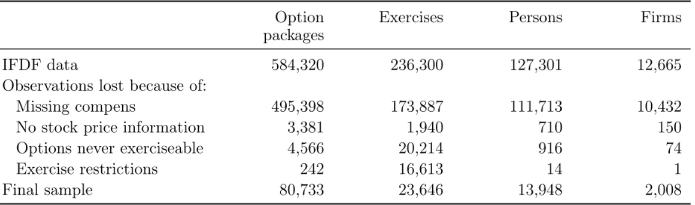
exer-cises not associated with stock sales separately as a robustness check. In total, we obtain 584,320 option packages associated with 236,300 exercises by 127,301 insiders. The steps of the construction of the sample are summarized in Table 1.
[Insert Table 1 about here.]
We match the IFDF data to the 2008 version of ExecuComp to obtain additional infor-mation about the executives themselves.10 From ExecuComp we obtain the beginning and the end of employment with the company, the fiscal year end, and annual data on total com-pensation, the sum of base salary and bonus, the Black-Scholes value of options granted, and the value of restricted stock granted. We lose 495,398 option packages because we cannot match them to ExecuComp, mostly because ExecuComp covers larger firms and only the top 5 managers, whereas IFDF also covers smaller firms and insiders other than the top 5 executives. Missing observations in dollar denominated variables in ExecuComp are set to zero.
We match these data with stock price data from CRSP. We lose another 3,381 option packages because we cannot match observations to CRSP or because there is no stock price information on CRSP for the relevant period. Finally, we are only interested in options that are potentially exercisable. We therefore omit all option packages (4,566 in total) that are out of the money for all data points we have between the vesting date and the maturity date. In our baseline specification and in Table 1 we count only exercises for at least 25% of the initial option package. (We consider other cutoffs later.) Because of these restrictions we lose 242 option packages and 16,613 exercises. Our final sample covers 80,733 option packages from 13,948 executives and 2,008 firms. For these options IFDF records 23,646 exercises of at least 25% of the initial grant.
We obtain annual dividend yields and dividend payment dates from CRSP. For firm-years with missing dividend information we set the dividend yield to zero. Additionally, we obtain dates of earnings announcements and accounting data from Compustat. The later hazard analysis will be based on weekly data. We therefore aggregate all exercises within the same week into one single exercise decision.
9For example, Aboody, Hughes, Liu, and Su (2008) obtain different results depending on whether they
study exercises after which shares are sold as opposed to exercises where shares are held.
10We can match by person names and firms’ CUSIPs. We match by first name, middle name, last name,
and name affix (“Jr.”, “Sr.”, etc.). Sometimes one database contains the affix, whereas the other database does not. In such cases, we match by first name, middle name, and last name. If the middle name is also not available in one database, then we match by first name and last name only.
[Insert Table 2 about here.]
The subjects of our analysis are option packages. Table 2 provides descriptive statistics for option packages at the vesting date for those options that are in the money for at least one week during the period between the vesting date and the earlier of the maturity date and the date until which we have data. Executive stock options are American options, hence we follow Heath, Huddart, and Lang (1999) and calculate option values using the model of Barone-Adesi and Whaley (1987), which accounts for the early exercise premium for American options when the underlying stock pays dividends. We refer to these values as BAW values from here on. For non-dividend paying stocks the BAW values coincide with the Black/Scholes values.11 We further report the time to maturity at the vesting date, the
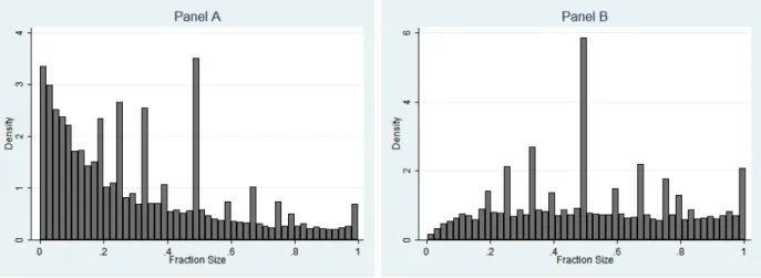
moneyness, the volatility based on returns for the past 52 weeks, the dividend yields at the end of the last calendar year, and the interest rate. For the interest rate we use zero coupon yields of zero-coupon government bonds with maturities of 1, 2, 3, 5, and 10 years and use the bond with a maturity that is closest to the maturity of the respective option. The value of option packages at the vesting date is $1.89 million on average (median: $0.35 million). Of the 80,733 option packages in our sample, 61,544 or 76% are in the money at the vesting date with an average stock price to strike price ratio of 18.48. (The median is only 1.32, a few firms have very large stock price increases between the grant date and the vesting date). The dividend yield of the firm is 1.43% on average and 0.85% for the median option package. Executives sometimes exercise only a fraction of the option package. Of the 33,283 ex-ercises in our sample, 58% are for a fraction of less than 100% of the initial grant, 43% are for less than 50%, 29% are for less than 25%, and 15% of all exercises are for less than 10% of the initial grant. In our baseline specification we count only the 23,646 exercises above 25% as economically meaningful. There are on average 1.31 exercises per option package for those packages where some options are exercised early. On average, 60% of an option package is exercised if at least some options are exercised early.
Figure 1 shows two histograms of the fraction sizes for partial exercises. In Panel A the bars in the histogram are proportional to the frequency of exercises for the particular fraction size, whereas in Panel B frequencies are weighted with the fraction size itself so that two exercises of 10% each have the same weight as one exercise of 20%. The pattern of fractional exercises reveals that executives prefer multiples of one fifth, one fourth, and one third of the initial grant. Note that this cannot be attributed to the structure of the grants
11A more appropriate model for risk-averse managers is probably Detemple and Sundaresan (1999).
How-ever, their model requires the knowledge not only of managers’ wealth, but also of the liquid portion of their wealth as well as assumptions about trading restrictions. We can therefore not implement their model with our data.
Figure 1: Partial exercises. The figure displays the frequency of fraction sizes for partial exercises. The fractions are calculated as parts of the total option package that was initially granted. Option grants with multiple vesting dates are broken up so that all options in the same package have the same vesting date. The bars in Panel A are proportional to the frequency of the fraction sizes, whereas the bars in Panel B are weighted with the fraction size itself.
themselves, which are sometimes staggered (equal fractions vest after 1, 2, and 3 years or similarly), since we ignore the exercises before the latest vesting date of such grants. (This deletion is inconsequential for our later analysis.) The histogram in Panel A is downward sloping, which implies that managers use smaller partial exercises more frequently than larger exercises. Panel B shows that, apart from the spikes noted above, the frequency of any fraction size is inversely related to the fraction size itself. This observation suggests that managers either exercise small portions of their option packages frequently, or larger portions, but then infrequently.
For the hazard analysis we use weekly data and exclude all weeks where an option package is out of the money.12 We only include options where the vesting date is available, so the
standard left censoring problem considered in hazard analysis (options where the beginning of their relevant lifetime cannot be observed) does not exist for our data set.13 However, for 31% of all option packages in our sample, we do not observe the grant date and there may be option packages that do not enter the database because their grant is not recorded on IFDF and they are not exercised early. We keep options without grant information in the data set and define the number of options granted as the number of options held at the first available transaction record or holdings record. For these options we potentially
12Exercising out-of-the-money call options is possible but irrational. For an analysis of irrational exercise
behavior for exchange traded options see Poteshman and Serbin (2003).
underestimate the total number of options granted and therefore overestimate the fraction that is exercised.14 Our later results show that the fraction of option grants that is exercised
does not have an impact on the results, so this measurement error seems inconsequential. Grant dates are not important for our analysis because for our purposes we count options’ lifetime from the vesting date and we retain the exercises of option packages without grant date as long as we know the vesting date.. Our study is therefore not affected by the fact that grant dates are sometimes missing, especially for those option packages that were granted earlier, presumably because the coverage of the database was then less complete.
[Insert Table 3 about here.]
Right censoring is present in our analysis whenever we have no record of the exercise of an option. Since multiple exercises per option package are possible, an option package may be right censored even if a fraction of it was exercised early. We are interested in early exercises only because they involve an economic decision by the manager. Exercises at maturity are outside the scope of our analysis because they result from the decision not to exercise earlier and are therefore covered indirectly by the analysis of early exercises. Hence, from the point of view of our analysis all options that are not exercised until one week before they expire are right censored.
Right censoring occurs also because insiders leave the firm. Usually insiders have to exercise their ESOs within a certain period of time after they leave the firm, otherwise their ESOs forfeit. However, the exact regulations also depend on the reasons why a manager left the firm. These rules are firm-specific and we do not have data on them.15 We therefore
take the date when an executive leaves the firm (which we obtain from ExecuComp) as the censoring date. All exercises after this date - some but not all of which are recorded on IFDF - are therefore not included in our data set. Observations are censored if insiders return options to the issuer because of repricings or if they dispose of them for other reasons. In the case of a repricing, the return of options to the issuer (cancellation) and the grant of new options with a lower strike price have to be filed with the SEC as separate transactions. However, repricings do not play a major role in our sample since they usually take place when options are out of the money. Finally, all options that are still alive at the end of December 2008 are right censored because the coverage of our version of IFDF ends on that date.
14Sometimes there are inconsistencies in the data and the number of options exercised exceeds the number
of options initially granted. In these cases we redefine the number of options granted as the total number of options exercised.
Table 3 shows the relative importance of right censoring reasons for our sample. If some portion of an option package is disposed of early (through exercises or gifts) while the remaining part is censored, we report the option package in the table as censored only if the larger part is censored. The major reason for right censoring (30.8% of the sample) is that the database records only exercises until December 2008. From the remaining 69.2%, only about one fifth of the options expire out of the money (12.4% of the whole sample) or get exercised at maturity (2.1% of the sample).
3
Methodology
We analyze stock option exercise patterns by CEOs and other insiders by using hazard analysis.16 To fix ideas, denote byf(t, x
t)the probability density function for the event that
the insider exercises her option package at time t, where xt is a vector of variables relevant
for the decision, which includes the characteristics of the option package, of the firm, of the market environment, and of the manager. Let F (t, xt) be the cumulative density function
associated with f. Then define the hazard rate h(t, xt) = f(t, xt)/(1−F (t, xt)) as the
conditional instantaneous probability that the insider exercises her stock options at time
t if she has not exercised (all of) them yet. Our definition of Exercise implies that the same option package can be exercised more than once (multiple spell analysis) and our econometric analysis accounts for this fact. We keep options in the analysis as long as at least an economically significant fraction of the number of options initially granted (25% in the baseline case) is left, otherwise the option package is censored.
The hazard approach offers major advantages.17 In particular, hazard analysis can easily
deal with censored data. Neglecting the right censoring in our data we mentioned above biases the estimate of the exercise probability downward because some exercise decisions are not observed. Restricting our analysis to uncensored observations would lead us to omit 78.5% of all option packages in the sample.18 Alternatively, we could estimate the conditional
16The discussion in this section is based on Kiefer (1988), Lancaster (1990), and chapters 17-19 of Cameron
and Trivedi (2005).
17Carpenter, Stanton, and Wallace (2008a) identify two limitations of hazard rate analysis. First, since the
unit of analysis are option grants, the analysis may miss out on cross-grant correlations. This is correct for the standard hazard rate approach, but does not apply to our analysis. Our model takes care of cross-grant correlations through a range of independent variables that model the option portfolio as well as firm-specific and individual-specific effects that may give rise to correlations. In addition, our model allows for random manager effects. Second, Carpenter et. al. argue that hazard analysis does not take into account fractional exercises. We take this into account by looking at a range of fractions to define the dependent variable. Almost all results are robust to this decision, but for choices from option portfolios small exercises are different from large exercises.
18The remaining 16.0% of the sample comprise the option packages that are exercised at maturity (1.1%),
densityf directly, for example by way of a logit or probit model and then infer unconditional probabilities. However, the dynamic logit approach cannot include censored observations.19
We proceed by using a proportional hazard model with piecewise constant baseline hazard as our baseline specification. The model is specified as follows:
h(t, xt) = λqexp{x0tβ}ν,
(1)
wherext is the time-varying vector of variables,λq are scalars for prespecified time intervals q, β is a vector of coefficients, and ν is a multiplicative random error that varies across individuals. The expression for h(t, xt) has three components.
The first component is λq and is referred to as the baseline hazard, which gives the
conditional probability of exercise when the other two factors both equal one. We seek the most flexible model for the baseline hazard, which does not impose any restrictions on the shape on the baseline hazard over time. For instance, the widely used Weibull model assumes a monotonic baseline hazard and violations of this assumption may bias coefficients. The second factor in equation (1), exp{x0tβ}, is the relative hazard, which multiplies the baseline hazard by a factor that depends on the variables xt. This factor is the core of our analysis.
The third component in (1) is the individual error term ν, which models unobserved heterogeneity. Unobserved heterogeneity is an important characteristic of our data. While we include a large number of variables in xt to control for as many effects as possible, there
are still individual factors that influence exercise decisions and which we cannot observe. These factors include preference parameters and unobserved manager characteristics like risk aversion or managers’ holdings of non-firm related assets. Ignoring unobserved heterogeneity when it is present can bias the estimates of the parameters of interest β. We therefore estimate a mixture model, where heterogeneity is modeled as a multiplicative individual error term ν that is common for all option grants of the same manager and distributed gamma.20 This specification is comparable to a random effects model for linear panel data and provides our main approach to model the correlation between observations for the same individual. In
in or before December 2008 (6.4%). The remaining 4.2% uncensored observations that make up the total of 10.6% reported in Table 3 mature after December 2008. Options that mature after December 2008 could not be included in a logit analysis because their lifetime is not always fully observable and becomes observable only if they are exercised.
19The hazard function approach does not estimate more or different parameters because parameterizing
the problem in terms of conditional or unconditional probabilities is equivalent (see Kiefer, 1988, p. 649). Shumway (2001) shows that the hazard function approach and a dynamic logit approach are identical if all observations where no failure event (here: option exercise) takes place are included in the analysis. He also shows that standard logit analysis will not provide correct standard errors.
20The specification is also known as a shared frailty model or a mixed proportional hazard model. See
Cameron and Trivedi (2005), chapter 18, for a discussion of unobserved heterogeneity and also for the discussion of alternative distributions of the error termν.
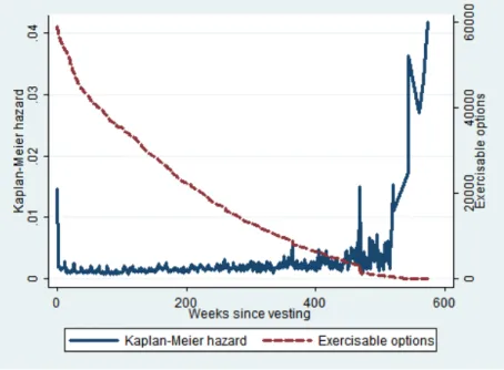
Figure 2: Empirical hazard rate. The solid line shows the non-parametric Kaplan-Meier estimate of the empirical hazard rate (left scale). This is the number of option packages with exercises of at least 25% of the original package, expressed as a fraction of all option packages that could have been exercised at that point in time. The dashed line (right scale) shows the number of option packages that could have been exercised.
one robustness check we report bootstrapped standard errors to make sure that our standard errors are not overstated because of other correlations. We have 13,948 individuals in our analysis, which precludes the use of individual fixed effects. We use weekly observations and estimate the baseline hazard for intervals of 13 weeks each.
Figure 2 shows the empirical hazard rate (solid line) as a function of time for our sample. For each week, it shows the ratio of the options exercised in that week relative to the number of unexercised options available at that point in time. The empirical hazard rate is non-monotonic. Exercise activity is very high immediately after vesting, and 10% of all exercised option packages are exercised, partially or fully, within two weeks of the vesting date. After vesting the empirical hazard rate drops to a lower rate, and finally increases again towards the end of the lifetime of the options. There are peaks in the hazard rate in annual intervals from the vesting date. We expect that this pattern is driven by annual events like grants of new options, vesting dates of existing options, and option expirations. Figure 2 shows the number of options that are still alive at any point in time. It takes 412 weeks from vesting (about 8 years) for this number to fall below 10%, and 469 weeks from vesting (about 9 years) to fall below 5% of the original sample. The empirical hazard rate becomes somewhat erratic more than ten years after vesting where data are scarce because only very few options are still alive.
4
Hypothesis development and analysis
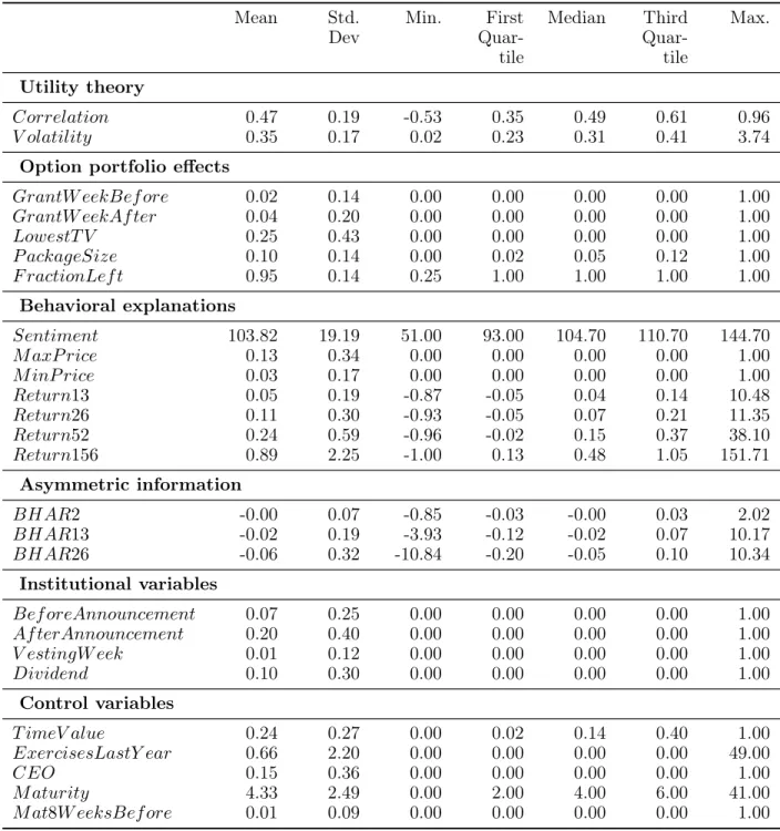
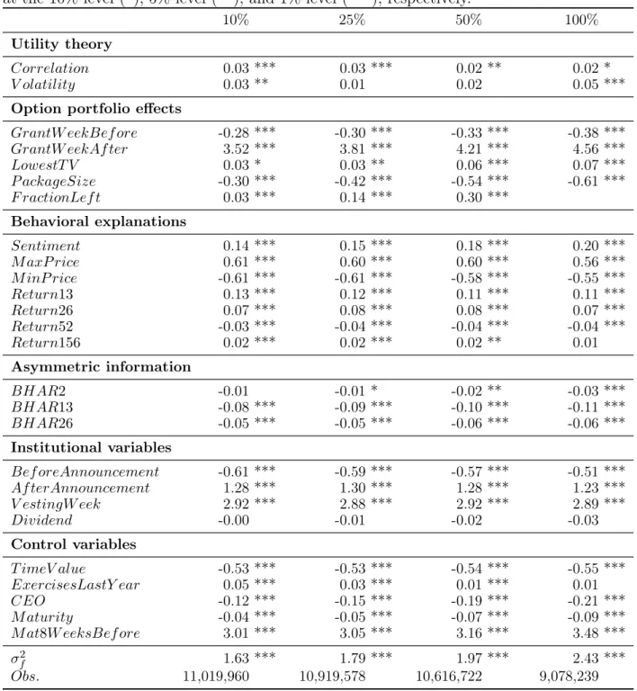
In this section we develop the hypotheses, grouped by the different explanatory approaches, i.e., utility theory, option portfolio effects, behavioral theories, and asymmetric information. We integrate hypothesis development with the presentation of the results for ease of ex-position. For each explanatory approach, we introduce the variables associated with each hypothesis and then immediately discuss the tests. Table 4 provides a detailed overview of all variables and their definitions. Table 5 presents descriptive statistics and Table 6 presents the estimation results for our hazard model.
[Insert Tables 4, 5, and 6 about here.]
Dependent variable: Exercise. The unit of investigation for our study is an option package. All options in one package have the same strike price and we use the longest vesting period and assign this vesting date to the whole package. Thus, exercises of the earlier vested portions of the grants are ignored. Alternative specifications (not reported) show that this choice is inconsequential for our results. The dependent variable in all our regressions is the dummy variableExerciset, which assumes a value of one if options in the
package are exercised at time t and zero otherwise. We report results for the event where the manager exercises at least 10%, 25%, 50%, or 100% of the options originally granted in one option package. Hence, Exerciset equals one if the fraction exercised as a percentage
of the initial package is at least as large as the respective threshold. Option packages for which less than this percentage is left are then dropped from the analysis. We often focus on results where the exercise threshold is set to 25%, which we treat as the baseline case, but always report the other specifications to document robustness.
We report relative hazards for individual variables as hri = exp{βi} −1 to facilitate
interpretation.21 We express all variables other than dummy variables as deviations from
their means, scaled by their standard deviations. Hence, if exp{βi} −1 equals 0.3, then this
implies that a one standard deviation increase in xi increases the probability of exercise in
week t by 30%. For the dummy variables exp{βi} −1 is simply the change in the hazard
rate if the dummy variable changes its value from zero to one.
21Conventionally, the relative hazard is defined asexp{βi}, which then has the interpretation of a factor.
Sinceβi ≈exp{βi} −1 for sufficiently small βi, our convention saves us from reporting separate tables for the coefficients.
4.1
Utility theory
Correlation. The starting point of utility theory is the observation that insiders exercise their stock options early because their investment in their own company’s securities exposes them to firm-specific risk. We measure the riskiness of the firm by two variables,Correlation
and V olatility. Correlation is the coefficient of correlation between the firm’s stock return and the return on the CRSP value weighted index. Correlation captures the idea that the manager can hedge the market risk of the stock by trading in the stock market, whereas she cannot hedge the idiosyncratic risk of the firm.22 We expect that managers exercise options
earlier if they find it more difficult to hedge their exposure, hence when the correlation with the market is lower. The coefficient onCorrelation should therefore be negative. We report robustness checks below for other variables that may capture the same effect, namely the firm’s beta and a measure of firm-specific risk.
The coefficient on Correlation is positive and statistically significant at the 1%-level for all definitions ofExercise. The value of the coefficient implies that a one-standard deviation increase inCorrelation increases the probability of exercise by 3%. We will show later that this result is robust to alternative definitions of idiosyncratic risk. This finding implies that executives behave in a way that is in direct contradiction to standard utility theory.
Volatility. The effect of the stock’s volatility on the decision to exercise early is ambiguous because volatility has two effects. Higher volatility makes the option more risky, so that a risk-averse manager would exercise early. However, volatility also increases the time value of the option. The first effect outweighs the second effect only if the manager is sufficiently risk-averse, so we cannot make an unambiguous prediction here. V olatilityt is defined as
the standard deviation of stock returns calculated over the 52 weeks preceding week t. The coefficient onV olatilityis small and positive. It is significant only at the 10% level, although it becomes more significant for exercise threshold of 10% and 100%. Our interpretation is that managers do wish to diversify their portfolios, but the diversification motive is almost outweighed by the countervailing effect on option values.
The results on Correlation and on Volatility contradict each other from the point of view of utility theory, since the latter suggest a moderate diversification motive, whereas the for-mer do not. However, these findings are consistent with rank-dependent preference theories, which predict that individuals combine diversified portfolios with undiversified holdings in
22Cai and Vijh (2005) and Carpenter, Stanton, and Wallace (2008b) present a utility-based models in
which the manager can invest in a risk-free asset, the firm’s stock, and the market portfolio. They show that managers value options subjectively higher when the the correlation between returns of the stock and the returns of the market portfolio is higher.
individual stocks (Polkovnichenko 2005, Barberis and Huang 2008). Polkovnichenko (2005) shows that consumers have such portfolios. We discuss this issue further in the Conclusion.
4.2
Option portfolio effects
New option grants. Managers may respond to the arrival of new option grants by exer-cising more of their existing options. This would always happen if managers have some target ownership of stock options, so that a new option grant increases their holdings above their target level.23 Managers may have such a target ownership because of portfolio
considera-tions or from stock ownership guidelines.24 From the point of view of utility theory, managers
would exercise their existing options if they receive a new grant simply because new option grants increase the exposure of the manager to firm risk. We includeGrantW eekBef ore, a dummy variable that equals one in the week before the manager receives a new option grant, and GrantW eekAf ter, a dummy variable that equals one in the week of and in the week after a new option grant. We expect the coefficients on both variables to be positive.
The coefficient on GrantW eekAf ter implies that the likelihood of exercising options in the week of or in the week after a new option grant is 381% higher than usual. By compari-son, the impact ofGrantW eekBef oreis negative, but has a lower impact in absolute terms. It is possible that we underestimate the last effect because we do not have grant dates for all option grants in our sample. If grant date information is not available the dummy variable is incorrectly set to zero for some observations, which biases the coefficient towards zero, hence the magnitudes of the effects we measure should be regarded as lower bounds. Also, reported grant dates may differ from actual grant dates if options are backdated (e.g., Heron and Lie, 2007). In this case, the negative effect of GrantDateBef oremay be contaminated by the positive effect of GrantDateAf ter if the week after the reported grant date is in fact the week before the actual grant date. Overall, this evidence is consistent with the notion that managers try to keep their option holdings at some target level.
Characteristics of the option portfolio. We capture the substitution between different packages the manager has available for exercise. The implicit assumption is that managers have decided to exercise some of their options for reasons explained by other factors, such as the motive to diversify or behavioral reasons, and they then select which option to exercise. We want to investigate how the characteristics of managers’ option portfolios affect their
23The results from Ofek and Yermack (2000) are consistent with the notion that senior managers have
ownership targets with respect to their stock holdings, so that they build up their ownership if it drops below this target.
24Core and Larcker (2002) analyze the impact of stock ownership guidelines for managers for a
selection among the options they have available. Managers always forgo some of the time value of the option, but we expect them to prefer exercising options with a lower time value.25
We define LowestT V to be one if the option package under consideration has the lowest time value of all available option packages. The coefficient on LowestT V is positive, but the economic as well as the statistical significance is marginal. Inference based on our regressions may be problematic for two reasons. First, we cannot directly infer whether managers make rational decisions conditional on exercising at least one option. The hazard regression estimates the conditional probability of exercise conditional on LowestT V = 1, whereas the question about the rational selection of options from a multi-option portfolio is about the probability that LowestT V = 1 conditional on exercise. While these two conditional probabilities are related through Bayes’ rule, inference on one cannot be linked directly to inference on the other. Second, the LowestT V is appropriate from the point of view of a risk-neutral agent, but may not properly reflect the trade-off between time-value and realized intrinsic value from the point of view of a risk-averse manager. A risk-averse manager may well resolve the trade-off between exercising a near-term, near-the-money option and a deep-in-the-money, long-term to maturity option with a similar time value differently compared to the prescriptions of a model that does not capture the exposure to firm-specific risk.
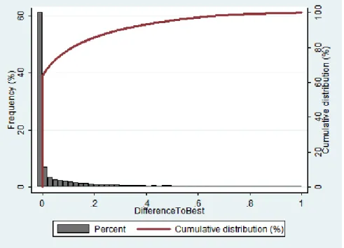
We address the first concern and further investigate the rationality of choices from multi-option portfolios. We define DifferenceToBest as the difference in time value between the option package managers actually select for exercise and the exercisable option package with the lowest time value.26 If managers select the optimal package, DifferenceToBest equals
zero, otherwise it is some positive number between zero and one because T imeV alue is also defined on the unit interval. We can therefore not include this variable in the haz-ard regressions. Figure 3 plots a histogram and the cumulative distribution function for
DifferenceToBest.
In 61.1% of all cases DifferenceToBest equals zero, which implies that managers choose the option with the lowest time value when exercising from a multiple-option portfolio. For 78.7% of all exercises DifferenceToBest is smaller than 0.10 and for 85.8% of all exercises it is smaller than 0.20. Hence, managers make errors when selecting which option package to exercise from, but they make predominantly small mistakes. Figure 3 also reveals that the likelihood of unnecessarily giving up time value declines rapidly as the size of the mistakes
25The only paper we are aware of that analyzes option portfolios is Grasselli and Henderson (2009). In
their model, managers exercise options with lower strike prices before they exercise options with higher strike prices. However, in their model options have infinite maturity so that time value and strike price are indistinguishable.
26If managers exercise multiple options simultaneously, then they naturally exercise options with a higher
time value as well. In this case DifferenceToBest is positive if they exercise options from a package while options from another package with a strictly lower time value remain unexercised.
Figure 3: Optimality of exercises. The figure shows a normalized histogram and the cumulative distribution of the variable DifferenceToBest, which is defined as the difference inT imeV aluebetween the option package with the lowestT imeV alueat the time of exercise and the T imeV alue of the option package actually chosen. The bars of the histogram are calculated as percentage frequencies.
increases. Regarding the second concern we note that the errors analyzed here may be still be overstated if DifferenceToBest does not adequately express the choice criterion of a risk-averse manager.
Small versus large exercises. We include P ackageSizejt, which is the Barone-Adesi
and Whaley (1987) value of all options in grant j that have not been exercised until time t, scaled by the value of the manager’s entire stock-dependent portfolio. Table 6 shows that the coefficient on P ackageSize is always negative and significant at the 1% level, but it depends on the exercise threshold. The coefficient decreases from -0.30 (threshold=10%) to -0.61 (threshold=100%). Hence, executives are more likely to exercise larger grants in smaller fractions, whereas they exercise smaller grants in larger fractions, which is consistent with the notion that managers have a target dollar value for option exercises.
We define F ractionLef tas the fraction of the initially granted option package that man-agers still hold and find that a one standard deviation increase in F ractionLef t (0.14 from Table 5) increases the probability of exercise by 14% in the baseline case. The coefficients on P ackageSize and F ractionLef t change as we increase the exercise threshold from 10% to 100%. These option portfolio effects depend on the exercise threshold, whereas all other
effects in Table 6 are more or less independent of how we define economically significant exercises.
4.3
Behavioral explanations
Investor sentiment. Many authors have documented the impact of investor sentiment on asset prices.27 We expect that stock option exercise decisions also respond to investor
sentiment. If managers behave like small retail investors, then they should invest more in risky stocks if investor sentiment is bullish and less if investor sentiment is bearish. Accord-ingly, we expect that managers who are subject to investor sentiment exercise their options later if investor sentiment is high. However, if managers are rational, they may recognize if prices are temporarily inflated (depressed) by retail investors subject to investor sentiment and may then exercise their options earlier (later).
For the purpose of our analysis we adopt the view of Lemmon and Portniaguina (2006) and use the consumer confidence index as an indicator of investor sentiment. In untabulated results we also use the sentiment indicator of Baker and Wurgler (2006) and obtain very similar results; we report the results for the consumer confidence index here because it is available for our entire sample period. We expect the coefficient onSentimentto be negative if managers behave like noise traders who believe that high sentiment indicates higher future stock prices, and we expect it to be positive if managers act like rational investors who believe that high (low) sentiment indicates that stock prices are temporarily inflated (deflated) and likely to revert to their fundamental levels. Our sample covers slightly more bullish option-weeks than bearish ones, with Sentiment having a median of 104.7 (mean 103.8), which is slightly above the neutral value of 100.
The coefficient on Sentiment is positive in all specifications and highly significant. A one-standard deviation increase in the consumer confidence index (19 index points) increases the probability of an early stock option exercise by 15% in our baseline case. This effect is therefore economically significant and contradicts the notion that managers are influenced by investor sentiment in their exercise decisions. Rather, they seem to see through investor sentiment and anticipate lower future returns when sentiment is high and vice versa. Hence, managers seem to take advantage of investor sentiment rather than being influenced by it.
Reference prices. The literature documents that individuals pay attention to the recent highs and lows of stock prices, which seem to anchor perceptions. These findings may result because individuals use extreme values of the stock price to form reference points
or simply because managers pay more attention to their stock when it breaches the past trading range.28 We follow this literature and include M axP rice and M inP rice in our
hazard regression. These are dummy variables, which equal one if the stock price in week
t is above its maximum, respectively minimum, over the preceding 52 weeks. We expect that individuals exercise their options more frequently if the stock trades above M axP rice
and less frequently if it trades below M inP rice. Consequently, the predicted coefficient on
M axP rice is positive and the predicted coefficient on M inP rice is negative.
The dummy variable M axP rice is consistently significant with positive coefficients, whereas the coefficients on M inP rice are always negative, as expected. The likelihood that managers exercise their options increases by 60% if their company’s stock trades above its 52-week maximum and the probability of exercise decreases by 61% if the stock trades be-low its 52-week minimum. This finding supports the notion that managers use salient stock prices like minima and maxima to form reference points, and then exercise their options if the stock trades above or below these reference points. However, our finding cannot rule out the alternative interpretation that managers are contrarian and pay more attention to their stock when it breaks out of its 52-week trading range (see Huddart, Lang, and Yetman’s (2009) study on volume and price patters in the stock market).
Trends in stock prices. Individuals seem to form beliefs based on the rule that short-term trends revert back to the mean, whereas long-short-term trends continue.29 If managers believe that a recent upward trend in their company’s stock reverts to the mean, then they believe that their stock is currently overvalued and it may be optimal for them to exercise the option and sell the stock now. We use four periodicities for past returns to explore the dependence of exercises on past returns, where we calculate returns over the last 13 weeks, 26 weeks, 52 weeks, and 156 weeks.
Our results are partially in line with the findings of Heath, Huddart, and Lang (1999) and support the notion that managers believe in mean reversion. The coefficients on Return13
and Return26 are all positive, significant at the 1%-level, and economically large. If the firm’s stock price increases by one standard deviation (19% in 13 weeks from Table 5) over the past three months, then the likelihood of exercising the option increases on average by
28Heath, Huddart, and Lang (1999) refer to prospect theory (Kahneman and Tversky, 1979) to motivate
the notion that individuals value their options by comparing the current stock price to a reference price. If the stock trades above this reference price, then individuals are risk-averse and exercise early. However, if the stock trades significantly below the reference price, then individuals become risk-seeking and defer exercising their options. Huddart, Lang, and Yetman (2009) argue that investors pay more attention to stocks when they break out of their 52-week trading range and offer evidence consistent with this hypothesis.
29To the best of our knowledge, Heath, Huddart, and Lang (1999) were the first to test this hypothesis for
stock option exercises. The findings on trends go back to Kahneman and Tversky (1973) and Tversky and Kahneman (1971).
12% in our baseline case. The results are similar but smaller for a 26-week interval.
By contrast, the results for long-term trend extrapolation are ambiguous. The coefficients onReturn52are negative, as expected based on the trend extrapolation hypothesis, whereas the coefficient on Return156 is positive, which is not in line with the results of Heath, Huddart, and Lang (1999). We performed an additional robustness check to make sure that these findings are not driven by the definition of returns, because the return variables overlap. If we define returns so that they are non-overlapping, then the results are very similar (results not tabulated).
The findings for all return variables exceptReturn156 are consistent with reference point behavior and the disposition effect, because managers seem to be more inclined to exercise options and sell stock when recent returns are positive and the stock trades above its recent high (“sell winners”), and hold on to options when the stock price has declined. This behavior may not be fully captured by the variables M axP riceand M inP rice (see Odean (1998) for a related interpretation of stock trading behavior). Reference dependence is therefore a more parsimonious explanation that may be sufficient to explain our findings on the stock-price dependence of managers’ exercise decisions except for very long-term returns, which can also not be explained by trend extrapolation.
4.4
Asymmetric information
Employees of the companies in our sample may have private information and exercise their options more often before negative news is disclosed, and less frequently before positive news is disclosed. Several authors find exercise patterns consistent with this notion.30 We proxy for inside information by calculating buy-and-hold abnormal returns for, respectively, 2 weeks, 13 weeks, and 26 weeks after week t. Testing for inside information by using realizations of ex post abnormal returns is standard in the insider trading literature (e.g., Lakonishok and Lee, 2001). If managers exercise options later because they expect positive news to materialize, or if they exercise earlier because they expect negative news to materialize, then the coefficients onBHAR2, BHAR13, and BHAR26should all be negative.31
We find that the coefficients on all buy-and-hold abnormal returns are significant and negative as predicted for all definitions of the dependent variable. Executives who exercise
30See Carpenter and Remmers (2001), Huddart and Lang (2003), Brooks, Chance, and Brandon (2007),
and Aboody, Hughes, Liu, and Su (2008). Bartov and Mohanram (2004) relate the stock price patterns around exercises to earnings management.
31We note that the abnormal returns subsequent to the average option-week are negative, which is puzzling.
We investigated this further and found that the average and the median BHAR are indistinguishable from zero for the firms in our sample. Hence, the negative BHARs for option-weeks arise because firm-weeks that are followed by negative BHARs are weighted with a larger number of options than firm-weeks followed by positive BHARs.
stock options and sell stock before the disclosure of bad news may violate insider trading rules, whereas those who delay exercises before the disclosure of good news do not. To inves-tigate this further, we split each BHAR-variable into a negative and a positive component (results not tabulated).32 We find that the resulting coefficients are very similar for the
neg-ative and the positive component of BHAR13 and BHAR26, but they differ significantly forBHAR2, where the negative component ofBHAR2has a positive sign: Managers avoid exercising their options and selling their stock shortly before negative news is released. The negative and the positive component of BHAR2 then partially cancel each other and the coefficient onBHAR2in Table 6 is accordingly much smaller and less significant than those on BHAR13and BHAR26. Our interpretation is that managers are less likely to exercise options if disclosures are imminent, irrespective of whether they reveal good news or bad news, probably to conform with insider trading prohibitions.
4.5
Institutional constraints and other control variables
Black-out periods. Most firms restrict trading of insiders by imposing black-out periods where insiders are not allowed to trade. Bettis, Coles, and Lemmon (2000) show that 92% of the firms in their sample impose such trading restrictions and that these trading restrictions lead to a significant decline in trading activity and a narrowing of bid-ask spreads for the firm’s stock. They show that a common window imposed for trading is 3 to 12 days after earnings announcements. Since we restrict our sample to option exercises where managers sell the shares they receive from exercises, we expect that trading restrictions around earnings announcements also affect exercise patterns. We capture this hypothesis with two variables,
BeforeAnnouncement, a dummy variable that equals one in the week before the earnings announcement, and Af terAnnouncement, a dummy variable that equals one in the week of and the week after an earnings announcement. If stock option exercises respond to trading restrictions for the company’s stock, then we expect the coefficient on BeforeAnnouncement
to be negative and the coefficient on Af terAnnouncement to be positive.
Trading restrictions because of blackout periods seem to be important. The coefficients onBeforeAnnouncement andAf terAnnouncementhave the predicted signs, are statistically highly significant, and economically large. In the week before earnings announcements, exercises are on average 59% below their normal rate in the baseline case. In the week after earnings announcements, exercises are 130% above their usual level. Our evidence therefore indicates that managers shift exercises from the period before earnings announcements to the period immediately after the announcement.
32More precisely, we define the two components asP osBHAR# =M ax(0, BHAR#)andN egBHAR# =
Vesting period. The vesting period prevents managers from exercising their options be-fore the vesting date. All theories we discuss above imply that managers sometimes wish to exercise their options early, so that the vesting constraint becomes binding. We therefore expect that managers exercise a significant portion of their options immediately after the op-tions vest, independently of the specific reason for early exercise. We include V estingW eek, a dummy variable that equals one in the week of and in the week after the option vests and we expect the coefficient on this variable to be positive. The coefficient on V estingW eek
implies that in the week of and the week after vesting, exercise rates are higher by 288%. This is consistent with the notion that the vesting constraint is binding. We can also observe the importance of the vesting restriction from Figure 2, which shows that the hazard rate is unusually high immediately after the vesting date.
Dividend capture. Managers may adjust their exercise strategies to their companies’ dividend policies if their options are not dividend protected (normally they are not). We therefore define Dividend as a dummy variable, which equals one in the week before and the week of a dividend payment. We expect the coefficient on Dividendto be positive. The coefficients on Dividend are statistically and economically insignificant. Our findings lend no support to the hypothesis that early exercises are driven by the desire to capture dividend payments. Dividend yields are typically low and are zero for more than half of our sample (see Table 2); they may therefore not play a major role.33
Time value. The time value of the option is relevant for all theories discussed above. All theories identify some benefit from exercising stock options early, such as benefits from diversification (utility theory), capturing temporary deviations of the stock price from its fundamental value (sentiment), or capturing a temporary informational advantage. The time value of the option, which is lost upon exercise, is the opportunity cost that managers trade off against the benefits from exercise. The relevance of the time value of the option therefore reveals something about the rationality of managers’ exercise decisions, but cannot help to discriminate among the different theories analyzed in this paper.
We therefore include the time value of the option as a control variable and define the variableT imeV alueas the time value of the option, divided by its Barone-Adesi and Whaley (1987) value.34 The time value of the option is a non-linear function of the
stock-price-to-33In other specifications (not tabulated) we also included the dividend yield and the exercise boundary of
the BAW-model. The dividend yield is also insignificant, and the coefficient on the BAW-boundary has the opposite (negative) sign of that implied by the dividend capture hypothesis.
34Some of the models based on utility theory explicitly identify exercise boundaries, where the benefits
from diversification exactly balance the time value, for example Huddart (1994) and Kulatilaka and Marcus (1994).
strike-price ratio. We prefer it to the stock price as an explanatory variable because the impact of the stock price may depend on the remaining term of the option, whereas the time value appears to reflect the economically relevant magnitude. However, we acknowledge that our definition of T imeV alue takes the perspective of a diversfied investor and not the perspective of a risk-averse manager (see also the related discussion of LowestT V above). Modeling the perspective of a risk-averse manager would involve additional assumptions about preferences, which we would not want to impose here. Also, in all likelihood the risk-neutral definition and a risk-adjusted definition would be highly correlated and lead to attenuation bias from the resulting errors-in-variables problem. T imeV alue can take values between zero for options that are close to expiration or deep in the money, and one for far out-of-the-money options. The coefficient on T imeV alue has the expected negative sign and is economically large. A one standard-deviation increase in T imeV alue reduces the likelihood of exercise by 53% in the baseline case, in line with all theories discussed above.
Heterogeneity across individuals. We need to model the time dependence of exercise decisions as current exercise decisions may depend on past exercises (occurrence dependence). We define ExercisesLastY ear as the number of exercises during the last 52 weeks. The coefficient on ExercisesLastY ear is positive. Hence, managers who exercised frequently last year also exercise small fractions of their grants more frequently this year. However, the effect is economically small and declines in the exercise threshold that defines the dependent variable.
Exercise behavior may depend on the status of the manager in the hierarchy of the firm. We distinguish between the CEO and the other top executives and include a dummy variable that equals one for CEOs. The coefficient on CEO is -0.15, so CEOs exercise options less frequently than other managers. In unreported results we run the model separately for CEOs and for non-CEOs to see if the impact of certain variables differs. We obtain similar results to the baseline case for both subsamples.
The variance σ2f measures the variation of the random effects ν in equation (1) in the model and it is significant in all specifications. Individual effects are therefore important and they are only partially captured by observed past exercise behavior and cannot be related to other observed characteristics. Other observables would potentially include managers’ age and their tenure on the job, but these are available only for a small subset of our sample.
Time and seasonal effects. We include M aturity, which is the remaining maturity of the option. Note that the baseline hazard is a function of the time since the vesting date, which is closely related. We define M aturity8W eeksBef ore as a dummy variable, which
equals one in the eight weeks before the maturity of the option and zero otherwise. The coefficients on both, M aturity and M aturity8W eeksBef ore confirm our expectation that there are more exercises close to maturity.
4.6
Overall evaluation
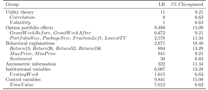
Contribution of explanatory approaches. In this section we evaluate the relative ex-planatory power of all variables in our analysis. In linear models we could develop a quan-titative benchmark by looking at partial R-squared measures, which are not available here. We attempt something similar for our hazard model by using likelihood ratio tests.
[Insert Table 7 about here]
In Table 7 we proceed as follows. Our baseline specification is again model (2) in Table 6. We then remove individual variables or groups of variables and perform a likelihood ratio test. The LR-test statistics in column (1) in Table 7 test for the joint significance for each group of variables in the table. For example, the test for “Utility” is for the joint exclusion of all variables suggested by utility theory, and the test for “V olatility” is for the exclusion of V olatility from the baseline model. Under the null hypothesis, the likelihood ratios are distributed Chi-square and column (2) reports the relevant cut-off values for the 1% significance level.
The quantitative importance of the variables specific to utility theory is very small. Moreover, the findings for Correlation contradict the predictions of utility theory. The findings for Volatility provide weak evidence for the diversification motive (see above) and we conclude that the diversification motive is poorly modeled by conventional utility theory. The explanatory power of the option portfolio effects is very large. These effects have not been studied before, but they are empirically more important than all other ap-proaches. The behavioral variables also have significant explanatory power, although it is much lower than those of T imeV alue, option portfolio variables, or institutional variables. It is attributable almost entirely to variables related to past stock returns. Variables related to asymmetric informationare significant at all conventional significance levels, but are quantitatively less important than those associated with any of the other explanatory ap-proaches. Finally, the variables representing institutional constraints are jointly of first-order importance.