Human Perception and Computer Graphics

Postgraduate Study Report DC-PSR-2004-06 Human Perception and Computer Graphics

Martin ˇCad´ık

Supervisor: Pavel Slav´ık January 2004

Department of Computer Science and Engineering Faculty of Electrical Engineering

Czech Technical University Karlovo n´am. 13

121 35 Prague 2 Czech Republic

email: [email protected] WWW: www.cgg.cvut.cz/~cadikm

This report was prepared as a part of the project

Perceptually Based Acceleration of Rendering

This research has been partly supported by the Ministry of Education, Youth and Sports of the Czech Republic under research program No. Y04/98: 212300014 (Research in the area of information technologies and communications).

. . . . Martin ˇCad´ık postgraduate student . . . . Pavel Slav´ık supervisor

Contents

1 Introduction 1

1.1 Organization of the Report . . . 2

2 Human Visual System 3 2.1 Physical Structure . . . 3

2.1.1 The Human Eye . . . 3

2.1.2 The Retina . . . 4 2.1.3 Visual Cortex . . . 6 2.2 Visual Perception . . . 7 2.2.1 Adaptation . . . 8 2.2.2 Ambiguous figures . . . 8 2.2.3 Visual Completion . . . 8 2.2.4 Impossible Objects . . . 9 2.2.5 Classification . . . 9

2.2.6 Attention and Consciousness . . . 9

2.3 Image Processing Theories . . . 10

2.3.1 Line and Edge Detection Theory . . . 10

2.3.2 Spatial Frequency Theory . . . 11

3 Perceptually Based Image and Video Quality Metrics 13 3.1 General Framework of Perceptual Quality Metrics . . . 13

3.2 Perceptual Image Quality Metrics . . . 14

3.2.1 Pixel-Based Metrics . . . 15

3.2.2 Model After Mannos and Sakrison . . . 15

3.2.3 Model After Gervais . . . 15

3.2.4 Visible Differences Predictor . . . 16

3.2.5 Perceptual Distortion Measure by Teo and Heeger . . . 18

3.2.6 Visual Discrimination Model . . . 18

3.2.7 Gabor Pyramid Model of the HVS . . . 19

3.2.8 Wavelet Visible Difference Predictor . . . 20

3.2.9 Multistage Perceptual Quality Assessment Model . . . 21

3.2.10 Metro: measuring error on simplified surfaces . . . 22

3.3 Video Quality Metrics . . . 22

3.3.1 Artifacts . . . 23

3.3.2 VQM by Lukas and Budrikis . . . 23

3.3.3 ST-CIELAB . . . 24

3.3.4 Moving Picture Quality Metric . . . 24

3.3.5 Perceptual Distortion Metric . . . 24

3.3.6 Non-Perceptual Metrics . . . 25

3.4 Conclusions and Future Research . . . 25

4 Perceptually Accelerated Rendering 26 4.1 Embedding HVS Characteristics Directly Into Algorithms . . . 26

4.1.1 Perceptually-Driven Radiosity . . . 26

4.2 Perceptual Metrics Operating on Rendered Images . . . 26

4.2.1 Perceptually Based Adaptive Sampling Algorithm by Bolin and Meyer . 27 4.2.2 Perceptually Based Physical Error Metric for Realistic Image Synthesis by Ramasubramanian et al. . . 27

4.3.1 Perceptual Convergence of Global Illumination Algorithms . . . 28

4.3.2 Hybrid Approach to Global Illumination . . . 28

4.3.3 Stopping Conditions for Global Illumination Computation . . . 29

4.4 Perception-driven Rendering of Animations . . . 30

4.4.1 Animation Quality Metric . . . 30

4.5 Conclusions . . . 30

5 Our Effort: Comparing Image-Processing Operators by Means of the Visible Differences Predictor 31 5.1 Non-Photorealistic Computer Graphics . . . 31

5.2 Motivation . . . 32

5.3 Comparison of Image-Processing Operators by the VDP . . . 32

5.3.1 Input scenes . . . 33

5.3.2 Tested techniques . . . 33

5.3.3 Comparison of the techniques . . . 34

5.4 Results . . . 34

5.4.1 Absolute values of differences . . . 34

5.4.2 Coherences . . . 36

5.5 Conclusions . . . 37

6 Conclusions 38

7 References 39

8 Dissertation thesis 43

9 Publications of the author 43

A Image Pyramids 44

Human Perception and Computer Graphics

Martin ˇCad´ık [email protected]

Department of Computer Science and Engineering Faculty of Electrical Engineering

Czech Technical University Karlovo n´am. 13 121 35 Prague 2 Czech Republic

Abstract

This report concerns human perception and its applications to the domain of computer graphics. Having in mind human perception limitations, we can design a perceptually opti-mized approach to virtually any issue of contemporary computer graphics. Such a perceptually optimized approach enable us either to visualize information more effectively and consequently to grasp important ideas and information from the depiction at a glance, or to save computa-tional time or improve the quality of results by removing perceptually non-important parts of visual simulation. Initially, we outline the anatomy of human visual system (HVS) and char-acteristics of human perception. Consecutively, we summarize the usage of HVS knowledge in computer graphics, we point out the bottlenecks of contemporary methods and we give the suggestions for future research. Specifically, we cover the issues of the image quality testing, the image comparison, and the acceleration of visual simulations and rendering. Finally, we present an experimental study on comparing image-processing operators.

Keywords

human perception, human visual system, computer graphics, image quality, vision models, image comparison, acceleration of rendering

1

Introduction

“The goal of computer graphics is not to control light, but to control our perception of light. Light is merely a carrier of the information we gather by perception.”

(Jack Tumblin, James A. Ferwerda)

Outputs of computer graphics are intended to be observed by human subjects. As human vision has several limitations, the knowledge of the human visual system (HVS) and of the human perception can be utilized to improve the performance of various computer graphics algorithms. In the field of computer graphics the knowledge of the human visual system usually takes the form of the computational models of human vision. Such a model can be incorporated at various areas of computer graphics.

One of the areas where the incorporation of human vision models is extremely beneficial is the image quality assessment and the image comparison. Image quality assessment and comparison metrics play an important role in various computer graphics applications. They can be used to monitor image quality for quality control systems, they can be employed to benchmark image processing algorithms, and they can be embedded into an image processing system to optimize the algorithms and the parameter settings. It is well known [49], that classical comparison metrics like Root Mean Square (RMS) error are not sufficient when applied to the comparison of images, because they poorly predict the differences between the images as perceived by the human observer. To solve the problem properly the visual differences predictors have evolved. The main part of visual differences predictors is typically a model of early vision, so that they perform well when comparing visually very near images. However their performance when comparing quite different images with respect to the contained information is poor. The predictor capable to incorporate such a behaviour would be valuable in the image database retrievals, to evaluation of the perceptual impact of different rendering algorithms, to analysis of the effect of various acceleration techniques, etc.

Alhough the progress in the computer hardware still persists, realistic image simulations and even computer generated animations are yet far away to be computed interactively. However, no matter how carefully we compute the displayed image, perception determines how much and how accurately we will understand what we see. Some visible difference predictors have been successfully applied to the fields of realistic image synthesis and synthetic animations, but most of current work in computer graphics does not consider any perceptual certainty. The search for means of utilization of human perception in rendering algorithms, realistic image synthesis, and computer animation, must go on.

The other problem is that much of the known HVS data has been obtained from specific psychophysical experiments which have been conducted in specialised laboratory environments under reductionistic conditions. These experiments were designed to examine a single dimension of human vision, however, evidence exists [39] to indicate that features of the HVS do not operate individually, but rather number of functions overlap and should be examined as a whole rather than in isolation. There is a strong need for the models of human vision currently used in image synthesis computations to be validated to demonstrate their performance is comparable to the actual performance of the HVS.

The goal of this report is to present specific properties of human visual system that are, or could be employed in computational models. Known visible differences predictors, their drawbacks and advantages are to be summarized. Consecutively, the overview of utilization of these predictors to the computer graphics rendering is to be given. Finally, the way to overcome drawbacks of contemporary approaches to the image comparison is to be outlined.

1.1 Organization of the Report

The report is organized as follows. Section 2 covers the physical structure and the perceptual behaviour of the human visual system. Section 3 summarizes the applications of human per-ception to computer graphics, namely to the field of image quality measurement. Section 4 describes usage of human perception in order to improve the rendering. Section 5 describes our contribution to the image comparison field. Section 6 concludes the report. Section 7 is the list of references and Section 8 gives the abstract of author’s prospective dissertation thesis. The appendix describes several widely used principles of method design and data analysis.

In this report, we do not cover the tone mapping field, which is concerned with the problem of mapping a bright scale of image luminances onto a narrow scale of display device in such a way that the perceived displayed image can be thought of as producing the same mental image as the original image. See the SIGGRAPH’03 Course #19 [10] for an overview. Furthermore, we

do not consider perceptual optimizations of 3D graphics and modeling, i.e. perceptual criteria for level of detail, and adaptive mesh subdivision and simplification, see outlines by Reddy [42] and the recent SIGGRAPH’03 Course #03 [13] respectively for a summary and references.

2

Human Visual System

Since the majority of perceptually based approaches to computer graphics is inspired by proper-ties of the human visual system, we will describe the HVS first. We will begin with the physical structure that is quite well estabilished and that can help us to understand rather complex char-acteristics of the perceptual behaviour. This part of the report was largely acquired from the excellent book on vision science by S. Palmer [39].

2.1 Physical Structure

In this section we will describe basic visual anatomy and physiology. This can give us insights into the kinds of information that can be coded by visual mechanisms.

2.1.1 The Human Eye

Humans have two eyes, which are approximately spherical in shape except for a bulge at the front. Located at about the horizontal midline of the head, they sit in nearly hemispherical holes in the skull, called the eye sockets. Each eye is moved by the coordinated use of six small, strong muscles, called the extraocular muscles, which are controlled by specific areas in the brain. Eye movements are necessary for scanning different regions of the visual field without having to turn the entire head and for focusing on objects at different distances.

iris lens cornea pupil aqueous humor optic nerve fovea retina ciliary muscles

Figure 1: A cross section of the human eye. (After Kolb et al. [24].)

The eyes have two important optical functions: to gather light reflected from surfaces in the world and to focus it in a clear image on the back of the eye. There are many parts of the eye that accomplish different optical functions, see Figure 1. First, light enters the cornea, a transparent bulge on the front of the eye behind which is a cavity filled with a clear liquid, called theaqueous humor. Next, light passes through the pupil, a variably sized opening in the opaqueiris, which gives the eye its external color. Just behind the iris, light passes through the lens, whose shape is controlled by ciliary muscles. The len’s optical properties can be altered by changing its shape, a process called accommodation. The photon then travels through the clear vitreous humor that fills the central chamber of the eye. Finally, it reaches the retina,

the curved surface at the back of the eye. The retina is densely covered with over 100 million light-sensitive photoreceptors, which convert light into neural activity.

The information about the light striking the retina is transmitted to the primary visual cortex in the occipital lobe at the back of the head, see Figure 2. Some estimates put the percentage of cortex involved with visual function at more than 50% in the macaque monkey, athough it is probably slightly lower in humans. The complete visual system includes much of the brain as well as the eyes, and the whole eye-brain system must function properly for the organism to extract reliable information about the environment.

Optic nerve Optic chiasm Lateral geniculate Optic radiations Visual cortex Superior colliculus

Figure 2: The human visual system. (After Palmer [39].)

2.1.2 The Retina

After the optics of the eye have done their job, the next critical function of the eye is to convert light into neural activity so that the brain can process the optical information. In the visual system, this function is carried out by photoreceptors in the retina: photoreceptors are specialized retinal cells that are stimulated by light energy. There are two distinct classes of photoreceptor cells: rods and cones. Rods are more numerous (about 120 million), extremely sensitive to light, and located everywhere in the retina except at its very center. They are used exclusively for vision at very low light levels (called scotopic conditions). Cones are less abundant (about 8 million), much less sensitive to light, and heavily concentrated in the center of the retina, although some are found scattered throughout the periphery. They are responsible for our visual experiences under most normal lighting conditions (called photopic conditions) and for all our experiences of colour. There is a small region, called the fovea, right at the center of the retina that contains nothing but densely packed cones. The visual angle covered by the fovea is only about 2 degrees. Another region exists where the axons of the ganglion

cells leave the eye at the optic nerve. This region is called the optic disk (also known as the blind spot) and it contains no receptor cells at all. However, we do not experience blindness there, except under very special circumstances.

Optic nerve fibers Ganglion cells Inner synaptic layer Amacrine cells Bipolar cells Horizontal cells Outer synaptic layer Receptor nuclei Receptors pigmented layer Light

Figure 3: The human retina. (After Palmer [39].)

Once the optical information is coded into neural responses, some initial processing is ac-complished within the retina itself by several other types of neurons, including thehorizontal, bipolar,amacrine, and ganglion cells, all of which integrate responses from many nearby cells, see Figure 3. The inputs of the retinal ganglion cells are arranged in an antagonistic, concentric pattern composed of a centre and a surround region (the area of the retina which the ganglion cell receives input from is called thereceptive field). The ganglion cell is continually emitting a background signal; however when light strikes the photoreceptors in one region, this stimulates an increased response from the retinal ganglion cell (on-response), whereas light falling on the other region will generate a reduced response (off-response). There are two distinct types of ganglion cells, theon-center cells, where the centre region is stimulated by an on-response, and theoff-center cells, where the centre region is stimulated by an off-response, see Figure 4.

The axons of the ganglion cells carry information out of the eye through the optic nerve to theoptic chiasm. Here the fibres from the nasal side of the fovea in each eye cross over to the opposite side of the brain while the others remain on the same side. The result is that the mapping from external visual fields to the cortex is completely crossed – all of the information from the left half of the visual field goes to the right half of the brain, while all the information from the right visual field goes to the left half of the brain. From the optic chiasm, there are two separate pathways into the brain on each side. The smaller one (only a few percent) goes to the superior colliculus, a nucleus in the brain stem. This visual center seems to process primarily information about where things are in the world and to be involved in the control of

+ -+

-A. On-center, Off-surround B. Off-center, On-surround

Figure 4: Receptive field structure of ganglion cells. On-center, off-surround cells (A) fire to light onset and stop at offset in their excitatory center, but they stop firing to light onset and begin firing at offset in their inhibitory sur-round. Off-center, on-surround cells (B) exhibit the opposite characteristics. (After Palmer [39].)

eye movements. The larger pathway goes first to the lateral geniculate nucleus (or LGN) of the thalamus and then to theoccipital cortex (or primary visual cortex).

2.1.3 Visual Cortex

The human cortex is divided into two halves, cerebral hemispheres, that are approximately symmetrical. As a result of many neuropsychological studies, it is now well estabilished that the occipital lobe is the primary cortical receiving area for visual information. Although it would be a gross overstatement to say that vision scientists understand how visual cortex works, they are at least beginning to get some glimmerings of what the assorted pieces might be and how they might fit together.

The first steps in cortical processing of visual information take place in the striate cortex, sometimes called primary visual cortex or area V1. This is the largest part of the occipital lobe and it seems likely that the most complex visual processing occurs there. Striate cortex receives its input from the LGN on the same side of the brain, so the visual input of striate cortex, like that of LGN, is completely crossed. Both sides are activated by the thin central vertical strip, measuring about 1 degree of visual field. The cells that are sensitive to this strip in one side of the brain are connected to the corresponding cells on the other side of the brain through thecorpus callosum, the large fiber tract that allows communication between the two cerebral hemispheres. The mapping from retina to striate cortex is topological in that nearby regions on the retina project to nearby regions in striate cortex. The central area of the visual field, which falls on or near the fovea, receives proportionally much greater representation in the cortex than the periphery does. This is called the cortical magnification factor.

The inferior temporal centers in the lower (ventral) system seem to be involved inidentifying objects, whereas the parietal centers in the upper (dorsal) system seem to be involved inlocating objects. These two pathways are often called the ”what” system and the ”where” system, respectively. It seems almost inevitable that these two different kinds of information must get together somewhere in the brain so that the ”what-where” connection can be made, but it is not yet known where this happens.

It is now abundantly clear that a great deal of visual processing takes place in parallel across different areas, each region projecting fibers to several other areas but by no means to all of them. The connections are generally bidirectional; that is, if area X projects to area Y, then Y projects back to X as well.

The Physiological Pathways Hypothesis

One possible relation between anatomical structure and physiological function has begun to emerge during the last decade. The hypothesis is that there are separate neural pathways for processing information about different visual properties such as color, shape, depth, and motion. Livingstone and Hubel [28] proposed that these four types of information are processed in different neural pathways from the retina onward. They report evidence that color, form, motion, and stereoscopic depth information are processed in distinct subregions of visual cortical areas V1 and V2, as indicated schematically in Figure 5.

Color Form Depth V2 Motion MT

Color Form Depth_Motion V1

Color

Form DepthMotion LGN

Color

Form DepthMotion RETINA

Figure 5: Schematic diagram of the visual pathways hypothesis.

These areas then project to distinct higher-level areas of cortex: movement and stereoscopic depth information to area V5 (also calledMT, Medial Temporal cortex), color to areaV4, and form through several intermediate centers (including V4) to area IT (InferoTemporal cortex), where cells have been found that respond selectively to faces, hands, and other highly complex stimuli. From these areas, the form and color pathways may project to the ventral ”what” system for object identification and the depth and motion pathways to the dorsal ”where” system for object localization.

2.2 Visual Perception

Visual perception is the process of acquiring knowledge about environmental objects and events by extracting information from the light they emit or reflect. Visual perception concerns the acquisition of knowledge – this means that vision is fundamentally a cognitive activity, distinct from purely optical processes such as photographic ones. There are indeed important similar-ities between eyes and cameras in terms of optical phenomena, but there are no similarsimilar-ities whatever in terms of perceptual phenomena – cameras have no perceptual capabilities at all. The knowledge achieved by visual perception concerns objects and events in the environment, perception is not merely about an observer’s subjective visual experiences. Visual knowledge about the environment is obtained byextracting information, that implies information process-ing approach to the vision. Finally the information that is processed in visual perception comes from the light that is emitted or reflected by objects, optical information is the foundation of all vision.

2.2.1 Adaptation

Visual perception changes over time as it adapts to particular conditions. When we enter a darkened room on a bright afternoon, for instance, we cannot see much. After 20 minutes, however, we can see everything surprisingly well. This increase in sensitivity to light is called dark adaptation. Adaptation is a very general phenomenon in visual perception – visual expe-rience may become less intense as a result of prolonged exposure to a wide variety of different kinds of stimulation: color, orientation, size, motion, etc. These changes in visual experience show that visual perception is not always a clear window onto reality because we have different visual experiences of the same physical environment at different stages of adaptation.

2.2.2 Ambiguous figures

To provide us with information, vision is aninterpretive process that somehow transforms com-plex, moving, two-dimensional patterns of light at the back of the eyes into stable perceptions of three-dimensional space. The objects we perceive are actually interpretations based on the structure of images rather than direct registrations of physical reality. Potent demonstrations of the interpretive nature of vision come from ambiguous figures, single images that can give rise to two or more distinct perceptions, see for an example Figure 6. The interpretations of these ambiguous figures aremutually exclusive. We perceive just one of them at a time: a duck or a rabbit, not both. This is consistent with the idea that perception involves the construction of an interpretive model because only one such a model can be fit to the sensory data at one time. If perception was completely determined by the light stimulating the eye, there would be no ambiguous figures because each pattern of stimulation would map onto a unique percept.

Figure 6: Ambiguous figures. Figure on the left can be seen as a duck (facing left) or a rabbit (facing right). Figure on the right can be seen as a saxophonist (facing right) or a face of a woman.

2.2.3 Visual Completion

People’s perceptions actually correspond to the models that their visual systems have con-structed rather than to the sensory stimulation on which the models are based. That is why perceptions can be illusory and ambiguous despite the nonillusory and unambiguous status of the raw optical images in which they are based. Perceptual models must be closely coupled to the information in the projected image of the world and must provide reasonably accurate interpretations of this information.

Perhaps the most convincing evidence that visual perception involves the construction of environmental models comes from the fact that our perceptions include portions of surfaces that we cannot actually see. This perceptual filling in of parts of objects that are hidden from

view is calledvisual completion. It happens automatically and effortlessly whenever we perceive the environment. Visual perception also includes information aboutself-occluded surfaces, those surfaces of an object thar are entirely hidden from view by its own visible surfaces.

2.2.4 Impossible Objects

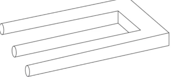
Impossible ojects are two-dimensional line drawings that initially give the clear perception of coherent three-dimensional objects but are physically impossible, see Figure 7. Such demon-strations support the idea that vision actively constructs environmental models rather than simply registering what is present. If visual perception were merely an infallible reflection of the world, a physically impossible object simply could not be perceived. The kinds of errors that are evident in perceiving impossible objects seem to indicate that at least some visual processes work initially at a local level and only later fit the results into a global framework.

Figure 7: Impossible object. The drawing in this figure produce perception of coherent three-dimensional object, but it is physically impossible.

2.2.5 Classification

Our perceptual constructions go even further than completing unseen surfaces. They include information about the meaning or functional significance of objects and situations. Beeing able toclassify objects as members of known categories allows us to respond to them in appropriate ways because it gives us access to vast amounts of information that we have stored from previous experiences with similar object. Previous experience with members of a given category allows us to predict with reasonable certainty what new members of the same class will do. As a consequence, we can deal with most new objects at the more abstract level of their category, even though we have never seen that particular object before.

2.2.6 Attention and Consciousness

The visible environment contains much more information than anyone can fully perceive. We must therefore be selective in what we attend to, and what we select will depend a great deal on our needs, goals, plans, and desires. Perception is not therefore an entirely stimulus-driven process – perceptions are not determined solely by the nature of the optical information present in sensory stimulation. Our perceptions are also influenced by cognitive constraints – higher-level goals, plans, and expectations. We look at different things in our surroundings depending on what we are trying to accomplish, and we may perceive them differently as a result.

One of the functions of attention is to bring visual information to consciousness. Certain properties of objects do not seem to be experienced consciously unless they are attended, yet unattended objects are often processed fully enough outside of consciousness to attract our attention. Once the object is attended, we become conscious of its detailed properties and

are able to identify it and discern its meaning in the present situation. In general, lower levels of perception do not seem to be accessible to, or modifiable by, conscious knowledge and expectations, whereas higher levels do. However not much is yet known about the role of consciousness in perception.

2.3 Image Processing Theories

Several theories for description of the nature of human image processing have evolved over the years. These theories compete because their functional implications are quite different and no one is universally held. We will describe the two most common of them: line–edge detection theory, and spatial frequency theory, although yet another approaches exist (connectionistic theory, neural networks, scale-space, etc.). Finally we will give an overview of contemporary theoretical hypothesis about the architecture of human image processing. This hypothesis integrates in some respect these two fundamentally different theories.

2.3.1 Line and Edge Detection Theory

Hubel and Wiesel [22] were the first to successfully apply the receptive field mapping techniques (described in section 2.1.2) to striate cortex. Their investigations revealed that there were several different kinds of cortical cells that had different receptive field characteristics. They classified them into three types: simple cells, complex cells,andhypercomplex cells. For simple cells, the responses to complex stimuli can be predicted from their responses to individual spots of light. A simple cell’s response to a larger, more complex pattern of stimulation can therefore be roughly predicted by summing its responses to the set of small spots of light that compose it. There were identified several different subtypes of simple cells. The vast majority have an elongated structure, firing most vigorously to a line or an edge at a specific retinal position and orientation. Simple cells that have an area of excitation on one side and an area of inhibition on the other, respond to a luminance edge in the proper orientation and are called edge detectors. Simple cells that have receptive fields with a central elongated region that is either excitatory or inhibitory, with an antagonistic field on both sides of it, respond maximally to bright or dark lines and are called line detectors orbar detectors.

The view of image processing that has emerged from these findings is that an early step in spatial image processing is to find the lines and edges in the image. Higher-level properties, such as shapes and orientations of objects, might then be constructed by putting together the many local edges and lines that have been identified by their detector cells in V1. Whether or not this is the correct view is still an open question, but it has dominated thinking about the initial stages of visual processing for several decades.

About 75% of the cells in striate cortex arecomplex cells. Similar to simple cells, complex cells have elongated receptive fields but they differ from simple cells in several important respects: complex cells are highly nonlinear, they tend to be highly responsive to moving lines or edges anywhere within their receptive field. Complex cells are not very sensitive to the position of certain stimuli and they tend to have somewhat larger receptive fields than simple cells. Complex cells are thought to receive input from several simple cells whose receptive fields have the same orientation but different positions.

The third type of striate cell is the hypercomplex cell. The most striking characteristic of hypercomplex cells is that extending a line or edge beyond a certain length causes them to fire less vigorously than they do to a shorter line or edge. For this reason, they are often called end-stopped cells. Recent quantitative studies suggest that the degree of ”end-stopping” is a continuum rather than an all-or-none phenomenon.

2.3.2 Spatial Frequency Theory

The spatial frequency theory dominates psychophysical theories of early spatial vision because it is able to explain a large number of important and surprising results from psychophysical experiments, not only in adult vision, but in infant vision as well. This theory is based on an atomistic assumption: the representation of any image, no matter how complex, is an assemblage of many primitive spatial ”atoms”. The primitives of spatial frequency theory are spatially extended patterns called sinusoidal gratings: two-dimensional patterns whose luminance varies according to a sine wave over one spatial dimension and is constant over the perpendicular dimension. Each primitive sinusoidal grating can be characterized completely by four parameters: itsspatial frequency, orientation, amplitude,and phase. Spatial frequency is usually specified in terms of the number of light/dark cycles per degree of visual angle. The orientation of the grating is specified in degrees counterclockwise from vertical. Phase is specified in degrees, such that the grating whose positive-going inflection point is at the reference point is said to have a phase 0◦ (called sine phase).

There is a good formal mathematical reason for choosing sinusoidal gratings as primitives: Fourier analysis. Fourier analysis is a method, by which any two-dimensional luminance image can be analyzed into the sum of a set of sinusoidal gratings that differ in spatial frequency, orientation, amplitude, and phase. The Fourier analysis of an image consists of two parts: the power spectrum and the phase spectrum. The power spectrum specifies the amplitude of each grating at a particular spatial frequency and orientation, whereas thephase spectrum specifies the phase of each grating at a particular spatial frequency and orientation. If all of these gratings at the proper phases and amplitudes were added up, they would exactly recreate the original image. Thus, Fourier analysis provides a very general method of decomposing complex images into primitive components, since it has been proven to work for any image. Fourier analysis is also capable of being ”inverted” through a process called Fourier synthesis so that the original image can be reconstructed from its power and phase spectra.

Spatial Frequency Channels

The spatial frequency theory proposes that early visual processing can be understood in terms of a large number of overlappingpsychophysical channels that are selectively tuned to different ranges of spatial frequencies and orientations. Thanks to many psychophysical studies of peo-ple’s detection and discrimination of grating stimuli [1], there is now a great deal of evidence to support this view.

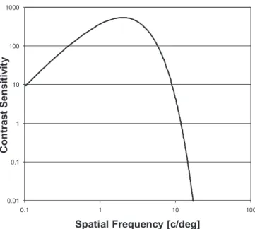
The standard measurement of human sensitivity to gratings at different frequencies is called thecontrast sensitivity function (CSF). It is determined by finding the lowest contrast at which the observer can just barely detect the difference between a sinusoidal grating and a uniform gray field, that is, the threshold at which a very low-contrast grating stops looking like a uniform gray field and starts to look striped. This threshold is measured for gratings at many different spatial frequencies from low to high. The results can be summarized in a graph in which the contrast sensitivity at threshold is plotted as a function of spatial frequency, as shown in Figure 8.

The CSF shows that people are most sensitive to intermediate spatial frequencies at about 4– 5 cycles per degree of visual angle. If the CSF is measured under low-light (scotopic) conditions in humans, sensitivity to all frequencies drops dramatically, especially at the highest frequencies. This means that at night, when just the rods are operating, human vision lacks the high acuity that it has in daylight.

Several measurements on human subjects have shown the selective adaptation of channels. The extended exposure to the grating caused the subject’s visual system to adapt, that is, to become less sensitive after the prolonged viewing experience (see section 2.2.1), but only near

0.01 0.1 1 10 100 1000 0.1 1 10 100

Spatial Frequency [c/deg]

C on tra st Se ns itiv ity

Figure 8: Contrast sensitivity function.

the particular spatial frequency and orientation of the adapting grating. Just as gratings of a particular spatial frequency and orientation produce specific adaptation effects, they also produce specificaftereffects.

Local Spatial Frequency Theory

Psychophysical channels are hypothetical mechanisms inferred from behavioral measures rather than directly observed biological mechanisms. If these channels are real, however, they must be implemented somewhere in the visual system. To face this problem there arises second theory about the function of the cells in striate cortex. There is now substantial evidence that these cells may be performing a local spatial frequency analysis of incoming images. A local, piecewise, spatial frequency analysis can be accomplished through many small patches of sinusoidal gratings that ”fade out” with distance from the center of the receptive field. This sort of receptive field structure, called a Gabor function, is constructed by multiplying a global sinusoidal grating by a bell-shaped Gaussian envelope, see the multiscale transforms introduction in the Appendix B.

The degree of frequency tuning in cortical cells seems to fall along a continuum; some are very sharply tuned and others quite broadly tuned. Cells that are tuned to high spatial frequencies have narrower tuning than do cells that are tuned to low spatial frequencies. There is a similar continuum in the degree of orientation tuning; some cells respond only to gratings that are very close to their ”favorite” orientation, whereas others respond almost equally to gratings in any orientation. Moreover, cells that are broadly tuned for spatial frequency are also broadly tuned for orientation, and cells that are narrowly tuned for spatial frequency are also narrowly tuned for orientation.

Although the evidence that simple and complex cells in area V1 may be doing a local spatial frequency analysis of input images is impressive, this conclusion is not universally held. Nev-ertheless, local spatial frequency theory must be counted a very serious alternative to the line and edge detection theory.

Architecture of Image Processing Hypothesis

We have reviewed two theories about the function of the cortical cells. The psychophysical view is that these cells describe images in a piecewise, local Fourier analysis. However, the edge detection theory claims that these same cells are actually the physiological implementation of edge detection mechanisms at different spatial scales. These different views are perhaps not as incompatible as they appear.

...

Frequency Analyzers Area V1 Center-Surround

Analyzers LGN

Edge

Analyzers CurvatureAnalyzers TextureAnalyzers MotionAnalyzers StereoAnalyzers

Figure 9: A theoretical hypothesis about the architecture of image processing.

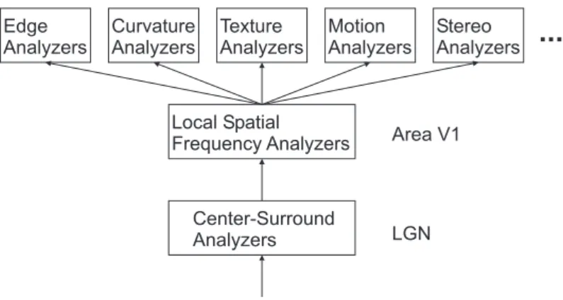
The hypothesis is that local spatial frequency theory and edge detection theory may be appropriate for different levels of the visual system, as diagrammed in Figure 9: center/surround cells in retina and LGN provide input to local spatial frequency analyzers in area V1 of visual cortex, which then project their output to a variety of different modules that compute edges, surface curvatures, textures, stereopsis, and so on, at later stages. According to this view, edge detectors would then be constructed from the output of local spatial frequency analyzers by coding for the output pattern that is characteristic of luminance edges.

3

Perceptually Based Image and Video Quality Metrics

In recent years a lot of effort has been given to the research of incorporation of human perception into the computer graphics and image processing methods. Thanks to this we have seen a big progress in several areas, e.g. in the field of image and video quality assessment. The goal of an objective image or video quality assessment is to develop quantitative measures that can automatically predict perceived image quality [54]. An objective image quality metric can play an important role in a broad range of applications, such as image acquisition, compression, communication, displaying, printing, restoration, enhancement, analysis and watermarking.

In this section we will first outline the general framework of quality metrics. Then we will summarize the perceptually driven image and video quality metrics that are or could be used in computer graphics. Finally, we will outline merits and shortcomings of these techniques. 3.1 General Framework of Perceptual Quality Metrics

A great variety of models has been proposed in the literature. For many of these models, common computational parts can be identified [55]. These parts are: preprocessing, CSF filtering, channel decomposition, error normalization and masking, and finally the error pooling, see Figure 10.

• The pre-processing stage may perform alignment, transformations of color spaces, cali-bration for display devices, point spread function filtering, and light adaptation.

Pre-processing CSFFiltering ChannelDecomposition ErrorNormalization and Masking Reference

signal Quality/Distortion

Measure Distorted signal Error Pooling .. . ...

Figure 10: Block diagram of typical discrimination/quality metric.

• CSF may be implemented before the channel decomposition using linear filters that ap-proximate the frequency responses of the CSF. Some metrics, on the other side, implement CSF as weighting factors for channels after the channel decomposition.

• Channel decomposition is used to model the frequency selective channels in the HVS. The channels serve to separate the visual stimulus into different spatial and temporal subbands. During this phase, quality metrics differ mostly in the chosen filters.

• Error normalization and masking is typically implemented within each channel. Most models implement masking in the form of a gain-control mechanism that weights the error signal in a channel by a space-varying visibility threshold for that channel. The visibility threshold adjustment at a point is calculated based on the energy of the signal in the neighbourhood of that point, as well as the HVS sensitivity for that channel in the absence of masking effects.

• Error poolingis the process of combining the error signals in different channels into a single distortion/quality interpretation. The typical implementation usesMinkowski summation (also called Lp-norm) on the two sets of channels to compute the model responser:

r= X l

X

k

|e_l,k|β1/β,

where el,k is the normalized and masked error of the k-th coefficient in thel-th channel, and β is a constant with a value between 1 and 4.

3.2 Perceptual Image Quality Metrics

Objective image quality metrics serve primarily to assessment of the difference between two images, an original image and a distorted image. They can be classified according to the availability of an original image, with which the distorted image is to be compared. Most existing approaches are known as full-reference, meaning that a complete reference image is assumed to be known. In many practical applications, however, the reference image is not available, and a no-reference or ”blind” quality assessment approach is desirable. In a third type of method, the reference image is only partially available, in the form of a set of extracted features made available as side information to help evaluate the quality of the distorted image. This is referred to as reduced-reference quality assessment.

Image quality metrics could be employed not only to image comparison, but also to accel-eration of rendering algorithms,perception-guided rendering of animations, etc., as one may see in Chapter 4. Since the visible differences predictor by Daly is extensively applied in the context of this report, it will be described more thoroughly.

3.2.1 Pixel-Based Metrics

The mean squared error (MSE) and the peak signal-to-noise ratio (PSNR) are the most pop-ular difference metrics in image and video processing. The MSE is the mean of the squared differences between the gray-level values of pixels in two picturesI and ¯I:

M SE= 1 XY X x X y [I(x, y)−I¯(x, y)]2,

for pictures of size X×Y. The average difference per pixel is thus given by the root mean squared error RM SE =√M SE.

The PSNR in decibels is defined as:

P SN R= 10 log m

2 M SE,

where mis the maximum value that a pixel can take (e.g. 255 for 8-bit images). Color PSNR is a version of the PSNR that accounts for colors, using perceptually uniform differences. Both MSE and PSNR are well-defined only for luminance information, there is no agreement on the computation of color values.

3.2.2 Model After Mannos and Sakrison

The first perception based image quality metric for luminance images was developed by Mannos and Sakrison [31]. Computation of the proposed model begins by normalizing all the luminance valuesLij by the mean luminanceLm. The nonlinearity in perception is accounted for by taking the cubed root of each normalised luminance. A Fast Fourier Transform is computed of the resulting values, and the magnitude of the resulting transform at frequencies in the horizontal and vertical directions (u, v),(whereuandvare expressed in terms of cycles per visual degree) is denotedfuv(||q3 L

Lm||).The magnitudesfuvare then filtered with the CSFAM(u, v) =AM(r),

where r = u2+v2 to account for spatial frequency sensitivity to produce the array of values

guv: AM(r(u, v)) = 2.6∗[0.0192 + 0.144 √ r] exp[−(0.144√r)1.1], guv=fuv(||( L Lm )0.333||)∗AM(r(u, v)).

Finally, the distance between the two images is computed by finding the Mean Square Error of the values guv for each of the two images:

M(X;Y) = 1

N X

all u,v

(gX,uv−gY,uv)2.

This technique therefore measures similarity in Fourier amplitude between images. It was shown to correlate quite well with subjective ranking data. Despite its simplicity, this metric was one of of the first works in engineering to recognize the importance of applying vision science to image processing.

3.2.3 Model After Gervais

Another simple model was adapted from a study of confusion between letters of the alphabet [15] by Rushmeier et al. [43]. The model includes the effect of phase as well as magnitude in the frequency space representation of the image. The luminances are normalised by dividing by the mean luminance. An FFT is computed producing an array of phases puv(||_LL

magnitudes fuv(|| L

Lm||) . The magnitudes are then filtered with an anisotropic CSF filter

function constructed by fitting splines to psychophysical data presented by Campbell et al. [5], producing the filtered valuesguv(||_LL

m||).The distance between images is then computed using: M(X;Y) = 1

N X

all u,v

(((loggX,uv+ 1)−(loggY,uv+ 1))(1 +pX,uv−pY,uv))2.

Since the Gervais model include phase (i. e. pixel position) information, its performance suffers due to subjectively minor registration problems between images. However, in situations where geometric alignment is not a problem, or is of critical importance for some other reason, this model may actually outperform the others.

3.2.4 Visible Differences Predictor

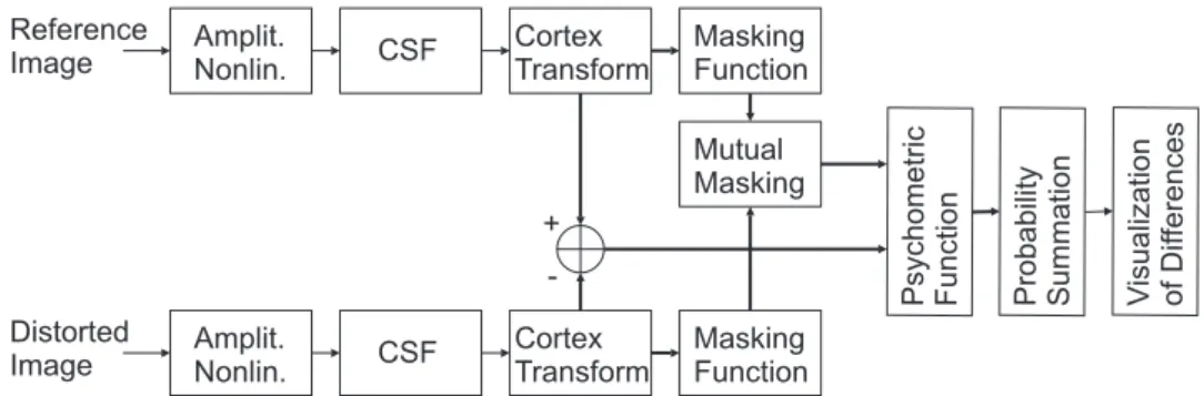
The Visible Differences Predictor [8] (VDP) is one of the best-known image distortion metrics. The VDP model interprets early vision behavior, from retinal contrast sensitivity to spatial masking. Figure 11 shows the use of the VDP, which consists of three main stages: components for calibration of the input images, a human visual system (HVS) model and a method for displaying the HVS visible differences. The input to the algorithm includes two images and parameters for viewing conditions, whereas the output is a map describing the visible differences between them (see Figure 22 on the page 31 for an example). The output map defines the probability of detecting the differences between the two images as a function of their location in the images. This metric, probability of detection, provides a description of the threshold behavior of vision but does not discriminate among different suprathreshold visual errors.

Amplit.

Nonlin. CSF CortexTransform MaskingFunction

Amplit.

Nonlin. CSF CortexTransform MaskingFunction Mutual Masking

Psychometric Function Probability Summation Visualization ofDif

ferences + -Reference Image Distorted Image

Figure 11: Block diagram of the Visible Differences Predictor (heavy lines indicate parallel processing).

Calibration

Firstly, the input images represented by unitless digital numbers are calibrated. The calibrating input parameters are: theviewing distance for which the VDP will make its visual prediction, and the physical pixel spacings, which along the viewing distance map the visual frequencies expressed in cycles per degree (c/deg) to frequencies expressed digitally as a fraction of the Nyquist frequency.

Human Visual System Model

The human visual system model is the key element of the VDP. It concatenates on the lower-order processing of the visual system, such as the optics, retina, lateral geniculate nucleus, and striate cortex. The HVS model consists of a number of processes that limit visual sen-sitivity. Three main sensitivity variations are accounted for, namely, as a function of light

level, spatial frequency, and signal content. Sensitivity S is defined as the inverse of the con-trast CT required to produce a threshold response, S = 1/CT, where contrast is defined as

C = (Lmax −Lmean)/Lmean, where Lmax and Lmean refer to the maximum and mean lumi-nances.

The variations in sensitivity as a function of light level are simulated byamplitude nonlin-earity. Each input luminance Lij is transformed by simplified version of the retinal response to an ”amplitude non-linearity value” bij defined as: bij = Lij/(Lij + 12.6L0ij.63), where the constants 12.6 and 0.63 apply when luminance is expressed in cd/m2. For this model the adaptation level for an image pixel is solely determined from that pixel.

The variations as a function of spatial frequency are modeled by the contrast sensitivity function, implemented as a filtering process. A Fast Fourier transform (FFT) is applied to the values bij. The resulting magnitudes, fuv(b) are filtered by a CSF which is a function of the image size in degrees and light adaptation level Lm.The resulting contrast sensitivity filter

AD(r(u, v)) is given by: AD(r(u, v)) = (0.008/r1.5+ 1)−0.21.42 √ rexp(−0.3√r) q (1 + 0.06 exp (0.3√r), where r=u2+v2.

The variations in sensitivity due to a signal content are reffered to as masking. Masking effects are modeled by the detection mechanism, which is the most complicated element of the VDP. It consists of four subcomponents: image channeling, spatial masking, psychometric function, and probability summation. Image channeling involves a decomposition similar to the cortex transform introduced by Watson [56]. Cortex transform is a multi-resolution pyramid (see Appendix A) that simulates the spatial-frequency and orientation tuning of simple cells in the primary visual cortex (see Section 2.3). During the image channeling stage, the input image is fanned out from one channel to 31 channels or bands as follows. Each channel is associated with one cortex filter which consists of aradial filter (dom, difference of mesa filter) and an orientational filter (fan filter). The total number of radial filters is six resulting in five frequency bands and one base band. Each of these bands except for the base band is further fanned out into six channels of different orientation, see Figure 12. Thus five frequency bands times six orientations per bands plus one base band results in 31 channels.

Radial frequency bandpass filters Orientation filters Baseband filter Input Image 1/2 1/4 1/8 1/16 1/32₀ cycles/pixel: 90° -90° -60° 30° 0° -30° 60°

Figure 12: Cortex transform. On the left: organization of the filter bank. On the right: decomposition of the image frequency plane into the radial and orientation selectivity channels.

Spatial masking reduces the detectability of a given stimulus through the simultaneous pres-ence of an additional suprathreshold stimulus. The masking depends on several factors, such as mutual masking, learning effects, the nature of masking signal, etc. Due to visual masking, threshold values can be elevated. This is accounted for after the transformation of all chan-nels back to the spatial domain. For every channel and for every pixel, the elevation of the

detection threshold is calculated based on the mask contrast for that channel and that pixel. Mutual masking can be considered by taking the minimal threshold elevation value for the corresponding channels and pixels of the two input images.

Psychometric function estimates the probability of detecting the differences for a given chan-nel. The applied psychometric function describes the increase in the probability of detection as the signal contrast increases. Once the detection probabilities have been computed for each band of the filter hierarchy, the probability images are combined into single image by pooling together probability contributions from all bands as a function of position.

Difference Visualization

There are two ways for visualizing the VDP output. The first technique is the free-field differ-ence map, where the visible differdiffer-ence predictions appear on a uniform field with a gray value near the system mean. The second method, the in-context difference map, is the mapping of the output probabilities in color on the reference image. It is assumed that the difference can be perceived for a given pixel when the probability value is greater than 0.75, which is a standard threshold value for discrimination tasks.

3.2.5 Perceptual Distortion Measure by Teo and Heeger

Teo and Heeger [49] presented a perceptual distortion measure based on the so-called normal-isation model – the nonlinear model of early phases of human vision. The model fits empirical measurements of the response properties of neurons in the primary visual cortext (see Sec-tion 2.1.3), and the psychophysics of spatial pattern detecSec-tion. In the primary visual cortex, a so-called contrast gain control mechanism keeps natural responses within the permissible dynamic range while at the same time retaining global pattern information. In the metric, contrast gain control is realized by an excitatory nonlinearity that is inhibited divisively by a pool of responses from other neurons. The channel decomposition process uses quadrature steerable filters with six orientation levels and four spatial resolutions. The distortion measure is computed from the resulting normalized responses by a simple squared-error norm to produce the difference map, similar to one produced by the VDP. Masking is modeled through contrast normalization and response saturation.

Authors in the paper [49] thoroughly demonstrate that the proposed measure is far better than the MSE and illustrate the usefulness of the model in measuring perceptual distortion in real images.

3.2.6 Visual Discrimination Model

The Sarnoff Visual Discrimination Model [29] (VDM) is another image discrimination metric. The overall structure of the model is outlined in Figure 13. The VDM operates in the spatial domain. First, the inputs are convolved with an approximation of the point spread function of the eye’s optics. The signals are then re-sampled to reflect the photoreceptor sampling in the retina. A Laplacian pyramid [4] (see Appendix A) is used to decompose the images into seven resolutions (each resolution is one-half of the immediately higher one), followed by band-limited contrast calculations. A set of orientation filters implemented through steerable filters of Freeman and Adelson [14] is then applied for orientation selectivity in four orientations. The CSF is modeled by normalizing the output of each frequency-selective channel by the base-sensitivity for that channel. Masking is implemented through a sigmoid non-linearity, after which the errors are convolved with disk-shaped kernels at each level. Finally, a distance measure or JND map is computed as the Lp-norm (Minkowski summation) of the masked responses.

Optics Bandpass Contrast Responses Oriented Responses Transducer Stimuli Sampling Qnorm JND Map Probability Distance JND Value

Figure 13: Block diagram of the Visual Discrimination Model.

The VDM is one of the few models that take into account the eccentricity of the images in the observer’s visual field. It was later modified to the Sarnoff JND metric for color video [57]. The complexity of Sarnoff VDM is O(N), because the VDM operates in the spatial domain and avoids expensiveF F T and F F T−1 transformations which take up to 40% of the execution time in the Daly VDP.

3.2.7 Gabor Pyramid Model of the HVS

Taylor et al. [48] presented a Gabor pyramid-based model of the human visual system (HVS) for image quality assessment. Their model departs from previous approaches in three ways:

• a physiologically and psychophysically plausible Gabor pyramid is used to model a recep-tive field decomposition

• psychophysical experiments are involved to directly assess the percept to be modeled

• the discrimination performance is modeled by using discrimination thresholds instead of detection thresholds.

A number of physiological studies have confirmed the hypothesis that mammalian visual systems contain neurons whose receptive fields closely resemble Gabor patches [48]. Because of the physiological and psychological plausibility of Gabor decomposition, the proposed model involves aGabor pyramid.

The model accepts two grayscale images as inputs and generates a probability map as out-put. A block diagram of the model is shown in Figure 14. A multiresolution decomposition is performed on each image to generate a number of channels, each containing the response of an ensemble of visual receptors. The receptors are modeled by Gabor functions of varying frequency and orientation. The multiresolution pyramid is built by lowpass filtering and deci-mating the original image, see Appendix A. Each output image for a particular pyramid level is called base image. The base image for each pyramid level is convolved with even and odd

Lowpass

Pyramid GaborWavelet

Psychometric LUT Lowpass Pyramid Channel Response Predictor Psychometric Selector + -Gabor Wavelet Masking Visible Difference Map Channel Summation Reference Image Distorted Image

Figure 14: Block diagram of the Gabor Pyramid Model.

symmetric Gabor wavelets at eight orientations. The square root of the sum of the squares of the resulting even-odd image pairs describes the response of an ensemble of neurons tuned to a particular spatial frequency and orientation. These images are called the channel images.

The Psychometric Look Up Table (LUT) consists of a family of psychometric functions that have been empirically determined by psychophysical experiments described below. The Psycho-metric Selector selects the appropriate psychoPsycho-metric function from the family of psychoPsycho-metric functions in the Psychometric LUT. A higher pyramid level base image determines the adapta-tion level, and the channel image determines the frequency, orientaadapta-tion, and reference contrast levels used to select the appropriate psychometric function. The difference between the contrast images for each channel is then applied to the appropriate psychometric function to produce a separate probability map for each channel. All of the probability maps from the different channels are combined using probability summation.

Two psychophysical experiments were conducted to determine the parameters of the model. The first experiment tested the visual system’s sensitivity to Gabor patches as a function of spatial frequency, orientation, and average luminance. The second experiment compared the relation between detection and discrimination thresholds.

3.2.8 Wavelet Visible Difference Predictor

Bradley’s [3] wavelet visible difference predictor (WVDP) is largely based on previously men-tioned (see Section 3.2.4) visible differences predictor, but has a number of modifications that make it more amenable to potential integration into a wavelet based image comparison scheme. These modifications include the use of aseparable wavelet transform instead of the cortex trans-form, the application of a wavelet contrast sensitivity function, and a simplified definition of sub-band contrast that allows prediction of noise visibility directly from wavelet coefficients, see Figure 15.

Another wavelet based metric has been proposed by Lai and Kuo [26]. Their metric is based on the Haar Wavelet and the masking model can account for channel interactions as well as suprathreshold effects.

Wavelet Transform Threshold Elevation Reference Image Wavelet Transform Probability Summation Distorted Image Mutual Masking + -Threshold Elevation VDM, Visible Difference Map Sub-band Detection Probability

Figure 15: Block diagram of the Wavelet Visible Differences Predictor.

3.2.9 Multistage Perceptual Quality Assessment Model

Multistage perceptual quality assessment model [38] (MPQA) was proposed to compare origi-nal and lossy compressed digital angiogram images. As shown in Figure 16, the MPQA model includes amplitude nonlinearity, octave bandwidth spatial frequency decompositions into six orientations using Watson’s cortex transformation [56], and contrast masking based on CSF modeling and region classification from the decomposed images. A perceptual distortion vis-ibility map (PDVM) is produced via a distance computation and summation of efforts across different spatial frequency bands. A perceptual quality rating (PQR) is then calculated from the PDVM converting fidelity to quality, and transformed into a one to five scale, PQR1−5.

Amplit.

Nonlin. SpatialFrequency Decomp. Contrast Map Region Classification Amplit. Nonlin. Contrast Error Map Contrast Masking (TE) + -Spatial Frequency Decomp. Contrast Map CSF Contrast Error Visibility Map Minkowski

Summation PerceptualDistortion Visibility Map Minkowski Summation Perceptual Quality Rating (1-5) Reference Image Distorted Image

Figure 16: Block diagram of the MPQA model.

As one may notice, the MPQA model is based on previously mentioned quality assessment models (mainly on the VDP, see Section 3.2.4), however it differs in the inclusion of contrast masking as a function of background uncertainty. The human eye can tolerate larger errors in high uncertainty simuli (i.e. in textured areas) than in low uncertainty stimuli of the same contrast (i.e. along edges). The spatially decomposed images are therefore classified into flat, edge, and texture regions to consider the relationship between stimulus and background uncertainty. Flat regions are the areas with lower contrast than the base threshold contrast

given by CSF. Edge areas are detected using a Sobel edge detector. Remaining regions are classified as texture regions. The threshold values are then elevated accordingly to the area type.

3.2.10 Metro: measuring error on simplified surfaces

Metro [6] is a tool that allows one to compare the difference between a pair of surfaces (e.g. a triangulated mesh and its simplified representation) by adopting a surface sampling approach. It has been designated as a highly general tool, and it does no assumption on the particular approach used to build the mesh representation. It returns both numerical results (meshes areas and volumes, maximum and mean error, etc.) and visual results, by coloring the input surface according to the approximation error.

Metro evaluates the difference between two meshes S1 and S2, on the basis of the approxi-mation error measure. The approximation error between two meshes is defined as the distance between corresponding sections of the meshes. Given a point p and a surface S, the distance

e(p, S) is defined as:

e(p, S) = min p0_∈Sd(p, p

0_),

whered() is the Euclidean distance between two points inE3. The one-sided distance between two surfaces S1, S2 is then defined as:

E(S1, S2) = max p∈S1

e(p, S2).

Given a set of uniformly sampled distances, the mean distance Em between two surfaces is defined as the surface integral of the distance divided by the area of S1:

Em(S1, S2) = 1

|S₁| Z

S1

e(p, S2)ds.

The error is evaluated by scan converting the first mesh faces with a user-specified sampling step, and computing a point-to-surface distance for each scan-converted point. The mean and maximum distances between meshes are returned.

Although Metro does not explicitly utilize any human visual system properties in the compu-tation, it has been used in several psychophysical experiments. Metro v.2 is available as public domain software at the Visual Computing Group web site of the CNUCE and IEI, C.N.R. Institutes at Pisa (http://miles.cnuce.cnr.it/cg/metro.html).

3.3 Video Quality Metrics

Assessment of video quality in terms of artifacts visible to the human observer is becoming very important in various applications dealing with digital video encoding, transmission, compression techniques, and computer graphics. Subjective video quality measurement is costly and time-consuming, and requires many human viewers to obtain statistically meaningful results. Several video quality metrics have been developed to face this problem.

Same as perceptual image quality metrics, the perceptual video quality metrics can save time by elimination of subjective testing. Moreover these metrics can help a lot when optimizing the storage space or download times of video clips. Applications of video quality metrics include:

• video encoder tuning and optimization,

• video security and watermarking,

In this section we will describe various artifacts that can occur in a video sequence. Consec-utively, we will give a brief overview on perceptually based video quality metrics.

3.3.1 Artifacts

We can distinguish a variety of artifacts in a video seguence [57]. Some of them may be caused by the compression algorithm, while the others occur as a consequence of transmission errors and various video conversions.

• Blockiness or the blocking effect refers to a block pattern in the compressed sequence. It is due to the independent quantization of individual blocks (usually 8×8 pixels) in block-based DCT coding schemes.

• Blur is characterised by the loss of fine detail and the smearing of edges in the video. It is typically caused by a high-frequency attenuation at some stage of the recording or encoding process. Wavelet-based encoders also cause blurry artifacts.

• Flickering appears when a scene has high texture contrast. Texture blocks are compressed with variyng quantization factors over time, which results in a visible flickering effect.

• Color bleeding is the smearing of the color between areas of strongly differing chrominance. It results from the suppression of high-frequency coefficients of the chroma components. Due to chroma subsampling, color bleeding extends over an entire block.

• Aliasing can be noticed when the content of the scene is above the Nyquist rate, either spatially or temporally.

• Mosquito noise is a temporal artifact seen mainly in smoothly textured regions as lumi-nance/chrominance fluctuations around high-contrast edges or moving objects. It is a consequence of the varied coding of the same area of a scene in consecutive frames of a sequence.

• When transporting media over noisy channelspacket loss orpacket delay can occur. Such losses or delays can affect both the semantics and the syntax of the media stream. A survey of video coding distortions can be found in an article by Yuen and Wu [58]. 3.3.2 VQM by Lukas and Budrikis

The first video quality metric was developed by Lukas and Budrikis [30]. It is based on a spatio-temporal model of the contrast sensitivity function using an excitatory and an inhibitory path. The two paths are combined in a nonlinear way, enabling the model to adapt to changes in the level of background luminance. Masking is also incorporated in the model by means of a weighting function derived from the spatial and temporal activity in the reference sequence. In the final stage of the metric, anLp-norm (Minkowski summation) of the masked error signal is computed over blocks in the frame whose size is chosen such that each block covers the size of the foveal field of vision. The resulting distortion measure was shown to outperform MSE as a predictor of perceived quality.

3.3.3 ST-CIELAB

Tong et al. [50] proposed a single-channel video quality metric called ST-CIELAB (spatio-temporal CIELAB). ST-CIELAB is an extension of the spatial CIELAB (S-CIELAB) image quality metric [59]. Both are backward compatible to the CIELAB standard, i.e. they reduce to CIEL∗a∗b∗for uniform color fields. The ST-CIELAB metric is based on a spatial, temporal, and chromatic model of human contrast sensitivity. The contrast sensitivity is modeled in an opponent color space, where the color information is encoded as white-black, red-green and blue-yellow color difference signals. After the CSF modeling, the data are transformed to CIE

L∗a∗b∗ space, whose difference formula is used for pooling. 3.3.4 Moving Picture Quality Metric

The Moving Picture Quality Metric (MPQM) proposed by Lambrecht [51] is a multichannel video quality model. It is based on a local contrast definition and Gabor-related (see Apendix B) filters for the spatial decomposition, two temporal mechanisms, as well as a spatio-temporal contrast sensitivity function and a simple intra-channel model for contrast masking. A color version of the MPQM based on an opponent color space was presented as well as a variety of appplications and extensions of the MPQM, e.g. for assessing the quality of certain image features such as contours, textures, and blocking artifacts, or the study of motion rendition.

Due to the MPQM’s purely frequency-domain implementation of the spatio-temporal filter-ing process and the resultfilter-ing huge memory requirements, it is not practical for measurfilter-ing the quality of sequences with a duration of more than a few seconds, however. The Normaliza-tion Video Fidelity Metric (NVFM) [27] avoids this shortcoming by using a steerable pyramid transform for spatial filtering and discrete time-domain filter approximations of the temporal mechanisms. It is a spatio-temporal extension of Teo and Heeger’s image distortion metric (see Section 3.2.5) and implements inter-channel masking through an early model of contrast gain control.

3.3.5 Perceptual Distortion Metric

Perceptual Distortion Metric (PDM), presented by Winkler [57], is a metric for both the digital color images and video. It is based on a contrast gain model of the HVS, which takes into account color perception, the multi-channel architecture of temporal and spatial mechanisms, spatio-temporal contrast sensitivity, pattern masking and channel interactions, see Figure 17.

Color Space

Conversion PerceptualDecomposition ContrastGain Control

Detection & Pooling Color Space

Conversion PerceptualDecomposition ContrastGain Control

Distortion Measure Reference Image Distorted Image

Figure 17: Block diagram of the PDM model.

The metric requires both the reference sequence and the distorted sequence as inputs. Both these sequences are converted to the opponent color space, where the color information is en-coded as white-black, red-green and blue-yellow color difference signals. After the conversion, each of the resulting three color components is subjected to a spatio-temporal filter bank de-composition. Temporal mechanisms are simulated by the temporal low-pass filter and by the