Andrade, Catherine. 2013. An Exploratory Study on Heads Up Photo Interpretation of Aerial Photography as a Method for Mapping Drainage Tiles. Volume 15, Papers in Resource Analysis. 14 pp. Saint Mary’s University of Minnesota University Central Services Press. Winona, MN 55987 Retrieved.
http://gis.smumn.edu
An Exploratory Study on Heads Up Photo Interpretation of Aerial Photography as a Method for Mapping Drainage Tiles
Catherine Andrade
Department of Resource Analysis, Saint Mary’s University of Minnesota, Winona, MN 55987
Keywords: Tile Drainage, Photo interpretation, Remote Sensing, Decision Tree Analysis, Aerial Photography, Iowa
Abstract
Agricultural producers have been using subsurface artificial drainage since the late 1800’s. This allows areas that would have otherwise been deemed unproductive for agriculture to grow substantial yields. Data and records on drainage tile location are not consistent. In recent years, researchers have turned to aerial photography to map
functioning drainage tiles. Knowing the location of drainage can allow more accurate hydrology studies. This research explores photo interpretation and compares it to remote sensing and decision tree analysis techniques to delineate subsurface agricultural drainage tiles in the Eagle Creek Watershed in Iowa, USA.
Introduction
Much of the Midwestern United States once contained numerous natural wetlands. Over the last 150 years agricultural producers have drastically altered the landscape by constructing subsurface tiles to drain these wetlands (Cooke, Badiger, and Garcia, 2001). The drained wetlands can be used as
agricultural lands producing substantial yields.
This network of drainage tiles bypasses natural riparian zones that once filtered the water. The drainage water contains nitrates, phosphorus, and pesticides from the agricultural fields and transports them directly to lakes and streams (Schilling and Helmers, 2008; Thompson, 2010; Goswami and Kalita, 2009; Bakhsh and Kanwar, 2008; Naz, Ale, and Bowling, 2009; Northcott, Verma, and Cooke, 2000).
Contamination of many impaired
waters throughout the Midwest can be attributed to artificial drainage systems (Green, Tomer, Di Luzio, and Arnold, 2006). Drainage from Midwestern states in the Upper and Central Mississippi River Basins accounts for 39% of the nitrogen delivered to the Gulf of Mexico (Bakhsh and Kanwar, 2008). As a result, hypoxic conditions are present in the Gulf (Bakhsh and Kanwar, 2008). Out of the 1,200 water bodies assessed by the Iowa Department of Natural Resources, 474 water bodies in Iowa were stated to have impaired water conditions (Iowa DNR, 2011).
Determining the location of agricultural drainage tiles would benefit and enhance the ecological planning process. Crumpton, Stenback, Miller, and Helmers (2006) show the potential benefits of wetland filters for tile drainage systems. They describe how constructed wetlands serve as nutrient sinks for the tile drainage water before
2 entering streams and rivers, as shown in Figure 1. Exact locations of drainage tile would aid in targeting locations for the constructed wetlands.
Figure 1. Outflow drainage tile. The photo was taken by Brian Phillips and used here with permission (North Carolina State University-Department of Biological and Agricultural Engineering, 2012).
The drainage network has resulted in multiple hydrological changes. Drainage tiles increase infiltration of precipitation, decrease evaporation, and lower the water table (Naz and Bowling, 2008). The
accumulation of water being directly transported from fields to streams has altered the natural stream flow (Schilling and Helmers, 2008) (Figure 2).
Tile effluent is the main water source into streams and rivers in
agricultural areas (Cooke et al., 2001). It is very important to understand how tile drainage affects the hydrology and land. Many hydrologic computer models attempt to simulate the affects. However, the drainage tile location is often
estimated. “APAPT, DRAINMOD, and RZWQM [hydrologic models] use parallel tile systems due to a lack of information about the location and characteristics of the drainage system and are sensitive to the spacing of the drains (Green et al., 2006).”
Figure 2. Agricultural drainage tiles in action. Used here with permission (Busman and Sands, 2002).
According to Northcott et al. (2000), most drainage tile patterns are random. Knowledge of the location of drainage tiles would lead to more accurate hydrology models and in turn lead to better hydrological monitoring and planning.
Study Site
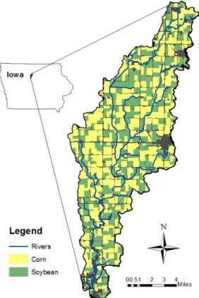
This study aims to locate drainage tiles at a watershed level. The Eagle Creek Watershed in Iowa USA is a
hydrological unit 10 watershed. The study area is mainly located in Wright County with the southern tip located in Hamilton County. According to the United States Department of Agriculture (USDA) National Agricultural Statistics Service, approximately 84.8% of Wright County land is planted with corn or soybean crops (USDA, 2007). Figure 3 shows the extent of corn and soybean in the Eagle Creek Watershed. Soybean and corn fields have the highest amount of drainage tiles (Thompson, 2010). Methods
Data
Photo Interpretation and Remote Sensing Data
3
Figure 3. Map of the study area showing corn and soybean crops.
Several aerial photographs of the Eagle Creek Watershed area were available, however only one was chosen as appropriate for detecting subsurface drainage. The reason this photograph was chosen was due to a significant rain event occurring before photo acquisition. This allowed visualization of different moisture levels in the soil directly above subsurface drainage. A color infrared two foot pixel orthophotograph taken April 29th, 2007 was used. This photo was publically available at the Iowa Natural Resources Geographic
Information Systems Library (Natural Resources Geographic Information Systems Library, 2012). Compliance with accuracy standards was ensured by the collection of airborne GPS data (Natural Resources Geographic Information Systems Library, 2012).
Rain data was obtained from the NOAA Advanced Hydrological
Precipitation Service (National Weather Service, 2012). Daily precipitation data was observed from 10 days prior to the photo acquisition date. This allowed for differences in rain fall across the Eagle Creek Watershed to be observed. The daily precipitation data was collected using radar and rain gauge data obtained from the National Weather Service and River Forecast Centers (National Weather Service, 2012).
Decision Tree Analysis Data
Several data layers were selected to be used for the Decision Tree Analysis. Soil characteristics, slope, and land use have often been used to define areas for artificial drainage (Naz and Bowling, 2008). The Iowa DNR published a layer for soils requiring tile drainage for full productivity (Natural Resources Geographic Information Systems Library, 2012). This layer will be
referred to as the SRTP. The SRTP layer incorporates soil characteristics as well as slope. The SRTP layer was created by combining two methods with data from the state-wide soils grid and the Iowa Soil Properties and Interpretations Database (Natural Resources Geographic Information Systems
Library, 2012). The first method defined the area meeting these criteria: a slope less than or equal to 2 degrees, drainage classes of poorly drained to very poorly drained soils, and hydrological group code of A/D, B/D, or C/D (See Appendix A; Iowa State University Extension and Outreach, 2010). The second method defined the area meeting these criteria: a slope of less than 5 degrees, a drainage code class of greater than 40, and a subsoil group of 1 or 2 (See Appendix B and C; Iowa State University Extension and Outreach,
4 2010). The grids from the two methods were joined by using a conditional statement. If method one was true, then the method one value was used.
Otherwise, the method two value was used. The final grid was then converted to a polygon layer and incorporated into the Decision Tree Analysis.
The land use dataset obtained was the 2007 Cropland Data Layer (CDL) from the National Agricultural Statistics Service (USDA, 2008). “The CDL was produced using satellite imagery from the Landsat 5 TM sensor, Landsat 7 ETM+ sensor, and the Indian Remote Sensing RESOURCESAT-1 (IRS-P6) Advanced Wide Field Sensor (AWiFS) collected during the current growing season (USDA, 2007b).” Analysis
Photo Interpretation/ Heads Up Digitizing
The image was visually scanned to detect differences in reflectance values in tile drainage fields. Digitizing was conducted at a 1:5,000 meter to 1:6,000 meter scale. Detected tile lines were manually digitized on-screen with the image as a background. This resulted in a line shapefile of tile lines. This method was a simple way to digitize drainage at a watershed scale without having substantial noise and it was less time consuming than probing the ground for the drainage tiles.
Precipitation Analysis
Remote sensing is a recent technique used to determine drainage tile locations (Naz and Bowling, 2008; Naz et al., 2009; Verma, Cooke, and Wendte, 1996; Northcott et al., 2000; Thompson, 2010).
However, this method is only applicable for assessment at a local scale. This technique has been shown to indicate drainage tiles with some level of accuracy (Naz and Bowling, 2008; Naz et al., 2009; Verma et al., 1996;
Northcott et al., 2000; Thompson, 2010). This part of the analysis was included to cross-validate photo interpretation findings with a more automated method.
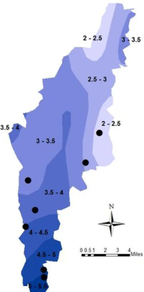
Since this remote sensing method was only applicable at a field level, a random point generator was used to find several sample points within the Eagle Creek Watershed. The points generated were applied to each precipitation class uniquely. This was carried out to assess how accurately drainage tiles were detected in areas receiving varying amounts of precipitation prior to the aerial photo. The daily precipitation values from NOAA came in point shapefile format. A spline interpolation was performed with the points to display approximate rain values throughout the Eagle Creek Watershed Area. The spline method was chosen because it resulted in the smoothest interpolation raster and it passed through the original input data points (ESRI, 2011). The interpolation raster was then reclassified into seven classes (Figure 4). The seven classes were categorized by half-inch intervals of the ten day rain totals. Next, the interpolation raster was converted to a polygon layer. A random point was created in each of the rain value class areas as sampling points. The field in which the random point was located was analyzed using the remote sensing methods. The fields range in size from 0.31 km2 to 1.35 km2.
Image Analysis
5 Classification tool was used to classify the image of each field into twenty classes based on pixel values.
Figure 4. Map of Eagle Creek Watershed with random sample points in each rain class. The rain classes are labeled with inches of total
precipitation. Darker blue refers to more rain fall where lighter blue indicates less rain fall.
Classification of twenty classes was successfully executed by Thompson (2010). The resulting rasters were overlaid with the aerial photograph and classes were categorized as associated with tile patterns. Whether or not a class was determined to be tile or non-tile was dependent upon each different
agricultural field. Each raster was
reclassified to a binary raster. The binary raster still needed to be cleaned up. The purpose of filters is to smooth the data by reducing local variation and
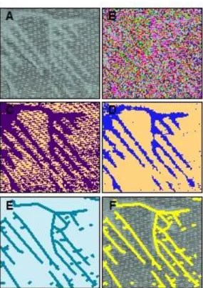
removing noise (ESRI, 2012). Previous studies had successful results with directional filters (Naz and Bowling, 2008; Naz et al., 2009); however when applied, directional filters created a fuzzy image and did not aid in the detection of tile drains. Multiple filters were experimented with on different fields. A 5x5 smooth filter resulted in cleaning up the most noise while preserving areas associated with drainage tile for all of the agricultural fields. The 5x5 smooth filter was applied to each binary image in this study. The rasters were then vectorized using ESRI software. Figure 5 displays image processing steps.
The photo interpreted line shapefiles were compared with the remotely-sensed tile lines. A ten meter buffer was generated around each field set of remotely-sensed tile lines. Ten meters was chosen due to the fact that the area of dry soil around tile lines is about twenty meters in width. If a ten meter buffer is applied to the centerline, in theory, the area of dry soil should be included. The percentage of photo interpreted tile lines that fell within ten meters of the remote sensing tile lines was determined by using the following formulas.
TLPIW10 = Total Length of Photo Interpreted Lines within 10 Meters of Remote Sensed Tile Lines
TLPI = Total Length of Photo Interpreted Tile Lines
X 100
Decision Tree Analysis
Decision tree analysis has been used as a starting point in many studies to
6
Figure 5. Image analysis process: A. Original image; B. Unsupervised classification with 20 classes; C. Tile/ Non-Tile reclassified raster; D. Image after smooth 5x5 filter; E. Vectorized tile lines; F. Tile lines overlaid on original image
However, in this study this information was used to validate the photo
interpretation tile layer. In the Crop Data Layer, the attributes of interest were the areas containing corn and soybeans. Soybean and corn fields have the highest amount of drainage tiles (Thompson, 2010). The Crop Data Layer was converted to polygon format and the corn and soybean areas were extracted for analysis. The SRTP layer
incorporated slope and soil
characteristics of tile drained areas and required no additional pre-processing. An intersect operation was performed with the corn and soybean layer and the SRTP layer (Figure 6) to incorporate areas containing all characteristics of tile drained land in this study area.
Descriptive statistics were performed using the formulas below to determine how many digitized tile lines
fell into areas that were characteristic of tile drained fields (Decision Tree
Classification Layer).
Figure 6. SRTP layer.
TLPIWDT = Total Length of Photo Interpreted Tile Lines that fall within the Decision Tree Classification Layer
TLPI = Total Length of Photo Interpreted Tile Lines
X 100
Results
Figure 7 illustrates the final photo interpretation tile map. Table 1 indicates percentages of the photo interpretation tile lines that fell within ten meters of the remotely-sensed tile lines. The accuracy
7 percentages generally showed a trend of increasing accuracy with increasing precipitation values. The exceptions were field 4 and field 6, which was very close to field 5 in accuracy percentage.
Table 1. The accuracy percentage is the percentage of photo interpretation tile lines that fall within ten meters of the remote-sensed tile lines. The rain values are shown to compare accuracy percentages for different agricultural fields. The rain value units are inches.
Field # Percentage Rain Value
1 25.7% 2-2.5 2 52.2% 2.5-3 3 54.8% 3-3.5 4 92.3% 3.5-4 5 74.1% 4-4.5 6 73.9% 4.5-5 7 89.1% 5-5.5
The Decision Tree Analysis indicated 88.8% of the photo
interpretation tile lines fell within areas that were consistent with characteristics of tile drained areas.
Discussion
Noise vs. Lost Data
One issue that was encountered in this study was the issue of noise vs. lost data when implementing remote sensing processing. Throughout the remote sensing process, it is beneficial to
remove as much noise/erroneous lines as possible for clarity. However, different image filters and vectorization settings, if set to remove noise, can also remove smaller tile lines or areas where tile lines are partially working. One area in the photo might have small areas of higher reflectance due to residue or tillage practices (Naz and Bowling, 2008). However, another area of the photo
Figure 7. Final photo interpreted tile map.
could have a small area of higher reflectance due to a partially working tile. The partially working tile may be erased depending on remote sensing settings. This issue was especially relevant when classifying the 20 unsupervised classes of reflectance values into a binary raster of tile and non-tile classification. Some of the 20 classes captured reflectance values of noise and partial tiles. Therefore, it was difficult to reclassify some of the initial classes. Unsupervised classification was used to keep the remote sensing methods as automated as possible in comparison to the photo interpretation methods. Rain Values
8 As mentioned, the usability of aerial
photographs to detect tile drainage is highly dependent upon the precipitation values in the days prior to the photo acquisition. This affects soil moisture during the time the photo is taken. The difference in soil moisture creates differences in reflectance values in the imagery and is how the tile is delineated. The Eagle Creek Watershed
precipitation classes were created to evaluate the accuracy of digitized lines as the precipitation values changes. The accuracy percentage gives an indication of how close the photo interpreted tile lines are in agreement with the remote-sensed tile lines. The accuracy
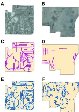
percentage showed an increasing trend as the rain values increased. The exceptions for this trend were fields 4 and 6. This gives cause to the argument that higher values of rain yield higher accuracy in delineating drainage tiles. Both the photo interpretation process and the remote sensing process depend on precipitation values to view the soil moisture. Accuracy percentages may have been lower in fields with less precipitation because the differences in soil moisture were so slight it was difficult for either process to differentiate tile lines (Figure 8).
Rain values in this study did not exceed 5.5 inches in the ten days before the aerial photo was taken. Therefore it is not known how much rain is too much or too little to detect drainage tiles. It is interesting to note that field 4 has a very high accuracy percentage. It may be that these tiles were recently constructed and in optimal working condition or
differences in soil may account for the high accuracy. This would require further investigation. More sample points in each rain class may validate the positive correlation between
precipitation values and accuracy of delineating drainage tile.
Figure 8. Differences in a high rain value field with a low rain value field. A. Original image of field 7; B. Original image of field 1; C. Photo interpreted tile lines for field 7; D. Photo interpreted tile lines for field 1; E. Remote-sensed lines for field 7; F. Remote-Remote-sensed lines for field 1.
Decision Tree Analysis
It was found that 88.8% of the photo interpretation tile lines fell into the area consistent with known characteristics of tile drained areas. This is a fairly high percentage and suggests photo
interpretation is a successful method to map agricultural drainage tiles.
Validating Findings/Existing Data The initial design of the study was to use remote sensing methods to cross-validate the photo interpreted lines. However, it
9 could be framed as the photo
interpretation method validating the remote sensing methods. In the end, both involve some human decision making. The automated process needs human intervention when classifying the twenty pixel classes as tile or non-tile.
Technology has not advanced enough to carry out a completely automated process. Also, more data on drainage records could solve the issue of validating the photo interpretation method as well the remote sensing method.
As mentioned, it is generally very difficult to find existing data on agricultural drainage tiles, especially at a watershed scale. Public agencies are trying to produce continuous data throughout the watershed. However, private fields and drainage systems are out of their jurisdiction. These field level drainage networks are still vital to increasing hydrological model accuracy. With cooperation of private land owners and location of private drainage
networks, photointerpretation techniques could be further validated. The mapping used in this study was in no way
connected to private owner information. Conclusion
In comparison with remote sensing techniques, the photo interpretation drainage tile lines generally showed improved accuracy with greater precipitation totals having occurred within the ten day period prior to the photo being taken. This suggests a higher rain value allows for the photo interpreted and remote-sensed tile lines to be in agreement. The photo
interpretation tile lines fell within the decision tree analysis area 88.8% of the time. These findings suggest photo
interpretation is a useful technique to map unknown drainage tiles. However, existing data or ground-truthing would validate these findings further.
Acknowledgements
I would like to thank the faculty at Saint Mary’s University, Ms. Greta Bernatz, Mr. John Ebert, and Dr. David
McConville, for sharing their
knowledge, time, and support. A special thanks to the La Crosse Fish and
Wildlife Conservation Office for sparking an interest in this subject and support for this tile mapping project. I also would like to thank JC Nelson for his continuous mentoring and advice. References
Bakhsh, A., and Kanwar, R.S. 2008. Soil and Landscape Attributes Interpret Subsurface Drainage Clusters. Australian Journal of Soil Research, 46, 735-744. Retrieved September 20, 2012 from Minitex.
Busman, L., and Sands, G. 2002. Agricultural Drainage Issues and Answers. University of Minnesota Extension. Retrieved January 4, 2013 from http://www.extension.umn.edu/ distribution/cropsystems/dc7740.html. Cooke, R.A., Badiger, S., and Garcia,
A.M. 2001. Drainage Equations for Random and Irregular Tile Drainage Systems. Agricultural Water
Management, 48, 207-224. Retrieved October 18, 2012 from Minitex.
Crumpton, W.G, Stenback, G.A., Miller, B.A., and Helmers, M.J. 2006.
Potential Benefits of Wetland Filters for Tile Drainage Systems: Impact on Nitrate Loads to Mississippi River Subbasins. Final Project Report to U.S. Department of Agriculture. Retrieved
10 November 6, 2012 from
http://www.fsa.usda.gov/Internet/FSA_ File/fsa_final_report_crumpton_rhd.pd f.
ESRI. 2011. An Overview of the Interpolation Toolset. Retrieved February 6, 2013 from
http://help.arcgis.com/en/arcgisdesktop /10.0/help/index.html#//009z00000069 000000.htm.
ESRI. 2012. Convolution Function. Retrieved February 6, 2013 from http://help.arcgis.com/en/arcgisdesktop /10.0/help/index.html#/Convolution_fu nction/009t0000004s000000/.
Goswami, D., and Kalita, P.K. 2009. Simulation of Base-flow and Tile-flow for Storm Events in a Subsurface Drained Watershed. Biosystems Engineering, 102, 227-235. Retrieved September 20, 2012 from Minitex. Green, C.H., Tomer, M.D., Di Luzio,
M., and Arnold, J.G. 2006. Hydrologic Evaluation of the Soil and Water Assessment Tool for a Large Tile-Drained Watershed in Iowa. American Society of Agricultural and Biological Engineers, 49(2), 413-422. Retrieved September 20, 2012 from
http://naldc.nal.usda.gov/download/335 /PDF.
Iowa Department of Natural Resources (DNR). 2011. The FINAL 2010 Iowa list of Section 303(d) Impaired Waters. Watershed Monitoring & Assessment Section, Iowa Geological & Water Survey, Environmental Services Division, Iowa Department of Natural Resources. Retrieved November 27, 2012 from http://www.iowadnr.gov/ Portals/idnr/uploads/watermonitoring/i mpairedwaters/2010/Fact%20Sheet%2
0for%20Final-approved%202010%20list.pdf. Iowa State University Extension and
Outreach. 2010. ISPAID Database
Manual. Iowa State University. Retrieved December 6, 2012 from http://www.extension.iastate.edu/soils/i spaid.
Natural Resources Geographic Information Systems Library. 2012. Retrieved November 27, 2012 from http://www.igsb.uiowa.edu/nrgislibx/ National Weather Service. 2012.
Advanced Hydrological Precipitation Service. Retrieved November 9, 2012 from http://water.weather.gov/precip/ download.php.
Naz, B.S., and Bowling, L.C. 2008. Automated Identification of Tile Lines from Remotely Sensed Data. American Society of Agricultural and Biological Engineers, 51(6), 1937-1950.
Retrieved October 31, 2012 from Minitex.
Naz, B.S., Ale, S., and Bowling, L.C. 2009. Detecting Subsurface Drainage Systems and Estimating Drain Spacing in Intensively Managed Agricultural Landscapes. Agricultural Water Management, 96, 627-637. Retrieved September 20, 2012 from Minitex. North Carolina State
University-Department of Biological and Agricultural Engineering. 2012. Drainage Water Management Background. Drainage Water Management Online Advisory. Retrieved January 4, 2013 from https://www.bae.ncsu.edu/topic/draina geadvisory/background.php.
Northcott, W.J., Verma, A.K., and Cooke, R.A. 2000. Mapping
Subsurface Drainage Systems using Remote Sensing and GIS. An ASAE Meeting Presentation. Paper No. 002113. Retrieved November 8, 2012 from Minitex.
Schilling, K., and Helmers, M. 2008. Effects of Subsurface Drainage Tiles on Streamflow in Iowa Agricultural
11 Watersheds: Exploratory Hydrograph
Analysis. Hydrological Processes, 22, 4497-4506. Retrieved May 21, 2012 from Minitex.
Thompson, J. 2010. Identifying Subsurface Tile Drainage Systems Utilizing Remote Sensing Techniques. The University of Toledo. Retrieved September 24, 2012 from
http://etd.ohiolink.edu/view.cgi?acc_nu m=toledo1290141705.
USDA. 2007. Quick Stats. National Agricultural Statistics Service. Retrieved November 27, 2012 from http://quickstats.nass.usda.gov/results/4
C4714D6-EB9C-326E-B729-338223540F9B.
USDA. 2007b. National Agricultural Statistics Service, 2007 Iowa Cropland Data Layer Metadata. Retrieved November 8, 2012 from
http://www.nass.usda.gov/research/Cro pland/metadata/metadata_ia07.htm. USDA. 2008. National Agricultural
Statistics Service. 2007 Cropland Data Layer. USDA-NASS, Washington, DC. Retrieved November 12, 2012 from http://nassgeodata.gmu.edu/Crop Scape/.
Verma, A., Cooke, R., and Wendte, L. 1996. Mapping Subsurface Drainage Systems with Color Infrared Aerial Photographs. Retrieved October 30, 2012 from
12
Appendix A. Hydrologic Group. These hydrologic groups are used to estimate runoff from precipitation. Soils not protected by vegetation are assigned to one of four groups. They are grouped according to the intake of water when the soils are thoroughly wet and receive precipitation from long-duration storms. [The hydrologic group listed for complexes is the most limiting group of the soils identified in the map unit name (i.e., Ackmore = B and Colo = B/D; Ackmore-Colo complex = B/D).] Data was obtained from Iowa State University Extension and Outreach (2010).
Hydrologic Group
Description
Group A Soils having a high infiltration rate (low runoff potential) when thoroughly wet. These consist mainly of deep, well drained to excessively drained sands or gravely sands. These soils have a high rate of water transmission.
Group B Soils having a moderate infiltration rate when thoroughly wet. These consist chiefly of moderately deep or deep, moderately well drained or well drained soils that have moderately fine texture to moderately coarse texture. These soils have a moderate rate of water transmission.
Group C Soils having a slow infiltration rate when thoroughly wet. These consist chiefly of soils having a layer that impedes the downward movement of water or soils of moderately fine texture or fine texture. These soils have a slow rate of water transmission. Group D Soils having a very slow infiltration rate (high runoff potential)
when thoroughly wet. These consist chiefly of clays that have a high shrink-swell potential, soils that have a permanent high water table, soils that have a clay pan or clay layer at or near the surface, and soils that are shallow over nearly impervious material. These soils have a very slow rate of water transmission.
13
Appendix B. Drainage Code Class. These codes refer to the frequency and duration of periods of saturation or partial saturation during soil formation, as opposed to altered drainage, which is commonly the result of artificial drainage or irrigation but may be caused by the sudden deepening of channels or the blocking of drainage outlets. [The drainage class listed for complexes is the most limiting class of the soils identified in the map unit name (i.e., Ackmore = SP-P and Colo = P; Ackmore-Colo complex = P).] Drainage class abbreviations and code numbers assigned follow. Data was obtained from Iowa State University Extension and Outreach (2010).
Drainage Code Class 10 Excessive 15 Excessive-Somewhat excessive 20 Somewhat excessive 25 Somewhat excessive-Well 30 Well 35 Well-Moderately well 40 Moderately well
45 Moderately well-Somewhat poor 50 Somewhat poor
55 Somewhat poor-Poor 60 Poor
65 Poor-Very poor 70 Very poor
14
Appendix C. Sub Soil Group. [Subsoil group listed for complexes is the most limiting group of the soils identified in the map unit name (i.e., Steinauer = 1 and Shelby = 2; Steinauer-Shelby complex = 2). Data was obtained from Iowa State University Extension and Outreach (2010).
Sub Soil Group
Description
1 Subsoil texture about the same as surface soil texture, not more than 34% clay, and subsoil favorable for crop growth.
2 Subsoil moderately unfavorable for crop growth: slow permeability [35-40% clay content] or high plasticity.
3 Subsoil very unfavorable for crop growth: silty clay and clay textures, very slow permeability [>40% clay content], or high plasticity.