CHAPTER 2
Design and Analysis of Comparative
Microarray Experiments
Yee Hwa Yang and Terence P. Speed
2.1 Introduction
This chapter discusses the design and analysis of relatively simple comparative experiments involving microarrays. Some of the discussion applies to all the most widely used kinds of microarrays, that is, radiolabelled cDNA arrays on nylon mem-branes, two-color, fluorescently labeled cDNA or long oligonucleotide arrays on glass slides, or single color, fluorescently labeled, high-density short oligonucleotide arrays on silicon chips. The main focus, however, is on two-color complementary deoxyribonucleic acid (cDNA) or long oligonucleotide arrays on glass slides because they present more challenging design and analysis problems than the other two kinds. As subfields of statistics, the topics of design and analysis of microarray experiments are still in their infancy. Entirely satisfactory solutions to many simple problems still elude us, and the more complex problems will provide challenges to us for some time to come. Much of what we present in this chapter could be described as first pass attempts to deal with the deluge of data arriving at our doors. Questions come in a volume and at a pace that demands answers; we simply do not have the luxury of waiting until we have final solutions to problems before we get back to the biologists. A major aim of this chapter is to stimulate other statisticians to work with their local biologists on microarray experiments and to come up with better solutions to the common problems than the ones we present here.
2.2 Experimental design
Statisticians do not need reminding that proper statistical design is essential to ensure that the effects of interest to biologists in microarray experiments are accurately and precisely measured. Much of our approach to the design (and analysis, see later) of microarray experiments, takes as its starting point the idea that we are going to measure and compare the expression levels of a single gene in two or more cell populations.
The fact that, with microarrays, we do this simultaneously for tens of thousands of genes definitely has implications for the design of these experiments, but initially we focus on a single gene.
In this section, some of the design issues that arise with the two-color cDNA or long oligonucleotide microarray experiments are discussed. Designing experiments with radiolabelled cDNA arrays on nylon membranes or for fluorescently labeled, high-density short oligonucleotide arrays is less novel. Apart from the following brief discussion about probe design, and a few other remarks in passing, we will not discuss these two platforms in detail separately.
Any microarray experiment involves two main design aspects: the design of the array itself, that is, deciding which DNA probes are to be printed on the solid substrate, be it a membrane, glass slide or silicon chip, and where they are to be printed; and the allocation of messenger ribonucleic acid (mRNA) samples to the microarrays, that is, deciding how mRNA samples should be prepared for the hybridizations, how they should be labeled, and the nature and number of the replicates to be done. We focus on the second aspect, after making a few remarks about the first.
The choice of which DNA probes to print onto the solid substrate is usually made prior to consulting a statistician; this choice is determined by the genes with expression levels that the biologist wants to measure, or by the cDNA libraries (that is, the col-lections of cDNA clones) available to them. With high-density short oligonucleotide arrays, these decisions are generally made by the company (e.g., Affymetrix) pro-ducing the chips, although opportunities exist for building customized arrays. Many researchers purchase pre-spotted cDNA slides or membranes in the same way as they do high-density short oligo arrays. With short (25 base pair) or long (60–75 base pair) oligonucleotide microarrays, the determination of the probe sequences to be printed is an important and specialized bioinformatic task (see Hughes et al. (2001); Rouil-lard et al. (2001);http://www.affymetrix.com/technology/design/ index.affxfor a discussion). Similarly, many issues need to be taken into account with cDNA libraries of probes, and here we refer to Kawai et al. (2001).
Advice is sometimes sought from statisticians on the use of controls: negative controls such as blank spots, spots with cDNA from very different species (e.g., bacteria when the main spots are mammalian cDNA), or spots “printed’’ from buffer solution, or positive controls such as so-called “housekeeping’’ genes that are ubiquitously expressed at more or less constant levels, and genes that are known not to be in the target samples, which are to be spiked in to it. We note that commercially produced chips (e.g., by Affymetrix) have a wide range of controls of these kinds built in. The questions typically posed to statisticians concern the nature and number of such controls, and the use to be made of signal from them in later analysis. Some controls are there to reassure the experimenter that the hybridization was a success, or indicate that it was a failure, as the case may be. Others are to facilitate special tasks such as normalization (see Chapter 1) or to permit an assessment of the quality of the experimental results. Controls used with cDNA microarrays for normalization include the so-called microarray sample pool (see Yang et al. (2002b) and the ScoreCard
system from Amersham Biosciences). At this stage we don’t have enough experience to offer general advice or conclusions in design for controls as the full use of such control data in cDNA arrays is still in its early stages. Yet another cDNA spot design issue on which statisticians might be consulted is the replicating of spots on the slide, and we discuss this next.
Graphical representation
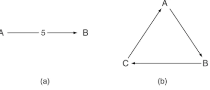
First, we introduce a method for graphical representation of microarray experimental designs. One convenient way to represent microarray experiments is to use a multi-digraph, which is a directed graph with multiple edges as illustrated in Figure 2.1(a). In such a representation, vertices or nodes (e.g.,A,B) correspond to target mRNA samples and edges or arrows correspond to hybridizations between two mRNA sam-ples. By convention, we place the green-labeled sample at the tail and the red-labeled sample at the head of the arrow. For example, Figure 2.1(a) depicts an experiment consisting of replicated hybridizations. Each slide involves labeling sampleAwith green (e.g., Cy3) dye, sampleBwith red (e.g., Cy5) dye and hybridizing them together on the same slide. The number “5’’ on the arrow indicates the number of replicated hybridizations in this experiment. Similar graphical representations of this nature have been used previously in experimental design, for instance, in the context of measurement agreement comparisons (Youden, 1969). For the rest of this chapter, we use this representation to illustrate different microarray designs. The structure of the graph determines which effects can be estimated and the precision of the estimates. For example, two target samples can be compared only if an undirected path joins the corresponding two vertices. The precision of the estimated contrast then depends on the number of paths joining the two vertices and is inversely related to the length of the path. In the hypothetical experiment presented in Figure 2.1(b), which consists of three sets of hybridizations, the number of paths joining the verticesAandB is 2; a path of length 1 runs directly betweenAandB; another path of length 2 joins AandBviaC. When we are estimating the relative abundance of target samplesA
Figure 2.1 Graphical representation of designs. In this representation, vertices correspond to target mRNA samples and edges to hybridizations between two samples. By convention, we place the green-labeled sample at the tail and the red-labeled sample at the head of the arrow. The number 5 denotes the number of replicates of that hybridization.
andB, the estimate oflog2(A/B)from the pathAtoBis likely to be more precise than the estimate oflog2(A/B)bylog2(A/C)−log2(B/C)from the path of length 2 joiningAandBviaC.
The preceding discussion assumes that the spot intensities in two-color experiments are all reduced to ratios before further analysis; however, it is already the case that some authors (Jin et al., 2001) are using single-channel data and not reducing to ratios. In this case, two strata of information exist on the log scale: the usual log-ratios within hybridizations, and log-ratios between hybridizations. Because of the novelty of this analysis approach, and the absence so far of a thorough discussion of single channel normalization, we concentrate our discussion of design and analysis to what it, in effect, is within the hybridization stratum (i.e., to analyses that depend on log-ratios within slides).
Optimal designs
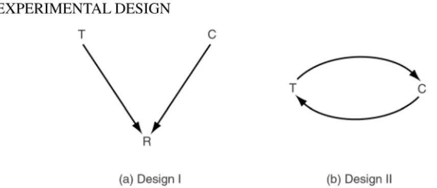
All measurements from two-color microarrays are paired comparisons, that is, mea-surements of relative gene expression, with microscope slide playing the role of the block of two units. We begin by discussing design choices for simple experiments comparing two samplesT andC. These include experiments comparing treated and untreated cells (e.g., drug treated and controls), cells from mutant (including knock-out or transgenic), and fromwild-typeorganisms (Callow et al., 2000), or cells from two different tissues (e.g., tumor and normal). Suppose that we wish to compare the expression level of a single gene in the samplesT andCof cells. We could compare them on the same slide (i.e., in thesamehybridization) in which case a measure of the gene’s differential expression could belog2(T/C), wherelog2Tandlog2Care measures of the gene’s expression in samplesT andC. We refer to this as adirect
estimate of differential expression—direct because the measurements come from the same hybridization. Alternatively,log2Tandlog2Cmay be estimated in twodifferent
hybridizations, withTbeing measured together with a third sampleRandCtogether with anotherRsample ofR, on two different slides. The log-ratiolog2(T/C)will in this case be replaced by the differencelog2(T/R)−log2(C/R), and we call this anindirectestimate of the gene’s differential expression because it is calculated with valueslog2Tandlog2Cfrom different hybridizations.
The early microarray studies (DeRisi et al., 1996; Spellman et al., 1998; Perou et al., 1999; and many others) performed their experiments usingindirectdesigns. These designs are also known as common reference designs in the microarray literature because each mRNA sample of interest is hybridized together with a common ref-erence sample on the same slide. The common refref-erence samples could be tissues fromwild-typeorganisms, orcontroltissue, or it could be apoolof all the samples of interest. Common references are frequently used to provide easy means of com-paring many samples against one another. More recently, several studies (Jin et al., 2001; Kerr et al., 2001; Lin et al., 2002) have performed experiments that provide
Figure 2.2 Two possible designs comparing the gene expression in two samplesT andCof cells. (a) Indirect comparison: This design measures the expression levels of samplesT and Cseparately on two different slides (hybridizations) and estimates the log-ratiolog2(T/C) by the differencelog2(T/R)−log2(C/R). (b) Direct comparison: This design measures the gene’s differential expression in samplesTandCdirectly on the same slide (hybridization).
and analysis of variance (ANOVA) have been used to combine data from the different hybridizations.
To date, the main work on design of two-color microarray experiments is due to Kerr and Churchill (2001), and Glonek and Solomon (2002), who have applied ideas from optimal experimental design to suggest efficient designs for some of the common cDNA microarray experiments. Kerr and Churchill (2001) based their comparisons of different designs on theA-optimality criterion. In addition, they introduced a novel class of designs they calledloopdesigns, and found that under A-optimality,loop
designs were more efficient than common reference designs.
Suppose we have a single factor experiment withKlevels and the goal is to compare allKtreatments. TheA-optimality criterion favors designs that minimize the average variance of contrasts of interest; however, this criterion alone is often not enough to single out one design; see Designs V and VI in table of Yang and Speed (2002). Just as different microarray experiments will require different analyses, no best design class suits all experiments. Frequently, the scientific questions and physical constraints will drive the design choices.
Glonek and Solomon (2002) studied optimal designs for time course and factorial experiments. Their article introduced classes of appropriate designs based on the notion ofadmissibility. For the same number of hybridizations, a design is said to be
admissibleif there exists no other design that has a smaller variance for all contrasts of interest. Their idea is that an investigator should compare only the admissible designs and then base their design selection on scientific interest. In Glonek and Solomon (2002) and in other similar calculations in the literature, log-ratios from different experiments are regarded as statistically independent. In the “Correlation and technical replicates’’ section, we revisit these calculations assuming a more realistic covariance between replicates, and we examine the implications for design optimality.
Design choices
In preparing to design a cDNA microarray experiment, certain general issues need to be addressed. These can be separated into scientific and logistic (practical). The scientific issues include the aim of the experiment. It is most important to state the primary focus of the experiment, which may be identifying differentially expressed genes, searching for specific patterns, or identifying tumor subclasses. Results from previous experiments or other prior knowledge may lead us to expect only a few, or many genes differentially expressed. In addition, there may be multiple aims within a single experiment, and it is important to specify the different questions and priorities between them. Practical or logistic issues include information such as the types of the mRNA samples, the amount of material and the number of slides (chips) available. The source of mRNA (e.g., tissue samples or cell lines) will affect the amount of mRNA available, and in turn the number of replicate slides possible.
Other information to keep in mind includes the experimental process prior to hybridiza-tion such as sample isolahybridiza-tion, mRNA extrachybridiza-tion, amplificahybridiza-tion and labeling. These and other technical matters are discussed in Schena (2000) and Bowtell and Sam-brook (2002). Keeping track of all the different aspects of the experimental process helps us better understand the different levels of variability affecting our microarray data. Finally, consideration should be given to the verification method following the experiments, such as Northern or Western blot analysis, real-time PCR, or in-situ
hybridization. The amount of verification to be carried out can influence statistical methods used and the determination of sample size. All this information helps us translate an experiment’s biological goals into the corresponding statistical questions and then, following appropriate design choices, helps us obtain a ready interpretation of the results.
We begin our discussion of the design of experiments when there is just one natural design choice, when one design stands out as preferable to all others, given the nature of the experiment and the material available. For example, suppose that we wish to study mRNA from two or more populations of cells, each treated by a different drug, and that the primary comparisons of interest are those of the treated cells versus the untreated cells. In this case, the appropriate design is clear: the untreated cells become a de facto reference, and all hybridizations involve one treated set of cells and the untreated cells. Next, suppose that we have collected a large number of tumor samples from patients. If the scientific focus of the experiment is on discovering tumor subtypes (Alizadeh et al., 2000), then the design involving comparisons between all the different tumor samples and a common reference RNA is a natural choice. In both cases, the choice follows from the aim of the study, with statistical efficiency considerations playing only a small role.
The statistical principles of experimental design are randomization, replication, and local control; naturally, these all apply to two-color microarray experiments, expe-cially the last two. We have so far found only limited opportunities for randomiza-tion, however, and the development of appropriate ways of randomizing microarray experiments would be a useful research project. In this and many similar laboratory
contexts, the challenge is to balance the requirements of uniformity (e.g., of reagents, techniques, technicians, perhaps even time of day for the experiment, which aims to reduce unnecessary variation, with the statistical need to provide valid estimates of experimental error). The situation recalls the discussion between R.A. Fisher and W.S. Gosset (“Student’’) in the 1930s concerning the relative merits of random and systematic layouts for field experiments; see Pearson and Wishar (1958) and Bennett (1971–1974) for the papers. A number of issues are highly specific to experimental design in the microarray context, and we now turn to a brief discussion of some of them. Parts of what follows will also be relevant to nylon membrane and high-density oligonucleotide arrays.
Replication
As indicated earlier, and consistent with statistical tradition (Fisher, 1926), replication is a key aspect of comparative experimentation, its purpose being to increase precision and, more important, to provide a foundation for formal statistical inference. In the microarray context, a number of different forms of replication occur. The differences are all in the degree to which the replicate data may be regarded as independent, and in the populations that experimental samples are seen to represent. Given that replicate hybridizations are almost invariably carried out by the same person, using the same equipment and protocols, and frequently at about the same time, it is inevitable that replicate data will share many features. Most of the differences discussed next concern the target mRNA samples.
Duplicate spots
Many groups spot cDNA in duplicate on every slide, frequently in adjacent posi-tions. At times, even greater within-slide replication is used, particularly with smaller customized rather than the larger general clone sets. This practice provides valuable quality information, as the degree of concordance between duplicate spot intensities or relative intensities is an excellent quality indicator; however, because replicate spots on the same slide, particularly adjacent spots, will share most if not all their experimental conditions, the data from the pairs cannot be regarded as independent. Although averaging log-ratios from duplicate spots is appropriate, their close asso-ciation means that the information is less than that from pairs of truly independent measurements. Typically, the overall degree of concordance between duplicate spots is noticeably greater than that observed between the same spot across replicate slides, although exceptions exist.
Technical replicates
This term is used to denote replicate hybridizations where the target mRNA is from the same pool (i.e., from the same biological extraction). It has been observed that
characteristic, repeatable features of extractions exist, and this leads us to conclude that technical replicates generally involve a smaller degree of variation in measurements than the biological replicates described next. Usually, the term technical replicate includes the assumption that the mRNA sample is labeled independently for each hybridization. A more extreme form of technical replication would be when samples from the same extractionandlabeling are split, and replicate hybridizations done with subsamples of this kind. We do not know of many labs now doing this, though some did initially. The section on “Correlation and technical replicates’’ discusses in more detail how technical replicates affect design decisions.
Replicate slides: Biological replicates—type I
This term refers to hybridizations involving mRNA from different extractions, for example, from different samples of cells from a particular cell line or from the same tissue. In most cases, this will be the most convenient form of genuine replication.
Replicate slides: Biological replicates—type II
This term is used to denote replicate slides where the target mRNA comes from the same tissue but from different individuals in the same species or inbred strain, or from different versions of a cell line. This form of biological replication is different in nature from the type I biological replicates described previously, and typically involves a much greater degree of variation in measurements. For example, experiments with inbred strains of mice have to deal with the inevitability of different mice having their hormonal and immune systems in different states, the tissues exhibiting different degrees of inflammatory activity, and so on. With non-inbred individuals, the variation will be greater still.
The type of replication to be used in a given experiment depends on theprecision
and on thegeneralizabilityof the experimental results sought by the experimenter. In general, an experimenter will want to use biological replicates to support the gen-eralization of his or her conclusions, and perhaps technical replicates to reduce the variability in these conclusions. Given that several possible forms of technical and biological replication usually exist, judgment will need to be exercised on the question of how much replication of a given kind is desirable, subject to experimental and cost constraints. For example, if a conclusion applicable to all mice of a certain inbred strain is sought, experiments involving multiple mice, preferably a random sample of such mice, must be performed.
Note that we do not discuss sample size determination or power in this chapter. Despite the existence of research showing how to determine sample size for microarray exper-iments based on power considerations, we do not believe that this is possible. Our reasons are outlined in Yang and Speed (2002).
Dye-swaps
Most two-color microarray experiments suffer from systematic differences in the red and green intensities which require correction. Details of normalization are discussed in Chapter 1. In practice, it is very unlikely that normalization can be done perfectly for every spot on every slide, leaving no residual color bias. To the extent that this occurs, not using dye-swap pairs will leave an experiment prone to a systematic color bias of an unknown extent. When possible, we recommend using dye-swap pairs. Alternatively, random dye assignments may be used, in effect including the bias in random error. A theoretical analysis of the practice of dye-swapping has yet to be presented.
Extensibility
Often, experimenters want to compare essentially arbitrarily many sources of mRNA over long periods of time. One method is to use a common reference design for all experiments, with the common reference being a “universal’’ reference RNA that is derived from a combination of cell lines and tissues. Some companies pro-vide universal reference mRNA (see e.g.,http://www.stratagene.com/gc/ universal mouse reference rna.html) while many individual labs create their own common reference pool. Common references provide extensibility of the series of experiments within and between laboratories. When an experimenter is forced to turn to a new reference source, it may be difficult to compare new experi-ments with previous ones that were performed based on a different reference source. The ideal common reference, therefore, is widely accessible, available in unlimited amounts, and provides a signal over a wide range of genes. In practice, these goals can be difficult to achieve. When a universal reference RNA is no longer available, it is necessary to carry out additional hybridizations, conducting what we term a linking experiment to connect otherwise unrelated data. More generally, linking experiments allow experimenters to connect previously unrelated experiments, with the number of additional hybridizations depending on the precision of conclusions desired. Suppose that in one series of experiments we used referenceR1, and that in another series we used referenceR2. The linking experiment comparesR1andR2, thus permitting comparisons between two sources, one of which has been co-hybridized withR1and the other withR2; however, this ability comes at a price. Log-ratios for sourceA co-hybridized with referenceR1can be compared to ones from sourceZco-hybridized with referenceR2, only by combiningA→R1andZ →R2together withR1→R2 through the identitylog2(A/Z) = log2(A/R1) + log2(R1/R2)−log2(Z/R2). In other words, cross-reference comparisons involve combining three log-ratios, with corresponding loss of precision, as the variance oflog2(A/Z)here is three times that of the individual log-ratios. Nevertheless, there will be times when cross-referencing is worthwhile, particularly when one notices that the variance of the linking term log2(R1/R2)can be reduced to an extent thought desirable simply by replicating that experiment. The linking term in the identity would be replaced by the average of all such terms across replicates.
Robustness
Loosely speaking, we call a design robust if the efficiency with which effects of interest are estimated does not change much when small changes are made to the design, such as those following from the loss of a small number of observations, or a change in the correlation structure of the observations. It is not uncommon for hybridization reactions to fail in microarray experiments; in a context where mRNA is hard to obtain, an experiment may well have to proceed without repeating failed hybridizations. In such cases, robustness is a highly desirable property of the design. A situation to be avoided is one where key comparisons of interest are estimable only when a particular hybridization is successful. It follows that heavy reliance on direct comparisons is not so desirable. Preferable is the situation where all quantities of interest are estimated by a mix of direct and indirect comparisons, that is, where many different paths connect samples in the design graph.
A nonstandard way to improve the robustness of a design is to give careful thought to the order in which the different hybridizations in the experiment are carried out. More critical hybridizations could be done earlier, and full sets of hybridizations com-pleted before further replicates are run, leaving the greatest opportunity for revising the design in the case of failed hybridizations. Note that this practice is contrary to the generally desirable practice of randomizing the order in which the parts of an experiment (here hybridizations) are carried out. In this context, such randomization is frequently achievable, but it is not popular with experimenters because it will often require a greater number of preparatory steps and so an increased risk of failure. As we will see later, the use of technical replicates introduces correlation between measured intensities and relative intensities. The precise extent of this correlation is typically difficult to measure. A design where the performance is more stable across varying technical replicate correlations would usually be preferred to one that is more efficient for one range of values of the unknown correlations, but less efficient for another range of values. This is a different form of robustness.
Pooling
An issue arising frequently in microarray experiments is the pooling of mRNA from different samples. At times pooling is necessary to obtain sufficient mRNA to carry out a single hybridization. At other times, biologists wonder whether pooling improves precision even when it is not necessary. Is this a good idea?
To sharpen the question, suppose that we wish to compare mRNA from source A with that from source B, using three hybridizations. We could carry out three separate extractions and labellings from each of the sources, arbitrarily pair A and B sam-ples, and do three competitive hybridizations, each a single A sample versus a single B sample. We would then average the results; see Section 2.3 (“Two-sample com-parisons’’) for further discussion. Alternatively, we could pool the labelled mRNA samples, one pool for the A and one for the B samples, then subdivide each pool into
three technical replicates, and carry out three replicate competitive hybridizations of pooled A versus pooled B. Again, the results of the 3 comparisons would be averaged. Which is better? An analogous question can be posed with the single-color hybridiza-tions (high-density short-oligonucleotide arrays, and nylon membranes). Ana priori
argument can be made for either approach. Pooling may well improve precision, that is, reduce the variance of comparisons of interest. But does it do so at the price of permitting one sample (or a few) to dominate the outcome, and so give misleading conclusions overall? These are hard questions to answer.
We know of no experiment with two-color microarrays aimed at answering these questions, but we have seen the results of such an experiment with the Affymetrix technology (Han et al., 2002). There we saw that averaging pooled samples and then comparing across the types described previously was slightly more precise than doing the same thing with averaged results from single samples, and in that case there seemed to be no obvious biases from individual samples. Our conclusion was that the gain in precision arising from pooling probably does not justify the risks, and that it is probably better to be able to see the between-sample variation, rather than lose the ability to do so. It remains to be seen whether this conclusion will stand up over time, and whether it applies to two-color microarrays.
Our design focus
With most experiments, a number of designs can be devised that appear suitable for use, and we need some principles for choosing one from the set of possibilities. The remainder of this chapter focuses on the question of identifying differentially expressed genes, and discusses design in this context. The identification of differ-entially expressed genes is a question that arises in a broad range of microarray experiments (Callow et al., 2000; Friddle et al., 2000; Galitski et al., 1999; Golub et al., 1999; Spellman et al., 1998). The types of experiments include:single-factor
cDNA microarray experiments, in which one compares transcript abundance (i.e., expression levels) in two or more types of mRNA samples hybridized to different slides. Time-course experiments, in which transcript abundance is monitored over time for processes such as the cell cycle, can be viewed as a special type of single-factor experiment with time being the sole single-factor. We discuss them briefly from this perspective. Factorial experiments, where two or more factors are varied across the mRNA are also of interest, and we discuss their design and analysis as well.
2.3 Two-sample comparisons
The simplest type of microarray experiment is the two sample or binary comparison, where we seek to identify genes that are differentially expressed between two sources of RNA. Such comparisons might be between knock-out and wild-type, tumor and normal, or treated and control cells. With “single color’’ systems, such as the nylon membranes and high-density short oligonucleotide arrays, the comparisons can be
between results from two arrays, or two sets of arrays. With the two-color cDNA or long oligonucleotide arrays, the comparison can be within a single slide, across each of a set of replicate slides involving direct comparisons, or involving indirect comparisons between slides.
Case Studies I and II
We illustrate the ideas of this section with two sets of two sample comparisons. These studies both aim to identify differentially expression between a mutant and a wild-type organism, but they do it differently. Both studies are with two-color cDNA microarrays. Case Study I involves replicates of direct comparisons made within a slide. By contrast, Case Study II involves indirect comparisons between samples co-hybridized to a common reference mRNA.
In order to identify and remove systematic sources of variation in the measured expres-sion levels and allow between-slide comparisons, the data for experiments I and II (as well as experiments III and IV introduced next) were normalized using the within-slide spatial and intensity dependent normalization methods described in Yang et al. (2002b). Normalization methods are discussed in more detail in Chapter 1, and we make no further mention of the topic, apart from noting that it is a critical preprocess-ing step with almost any microarray experiment.
Case Study I: Swirl zebrafish experiment
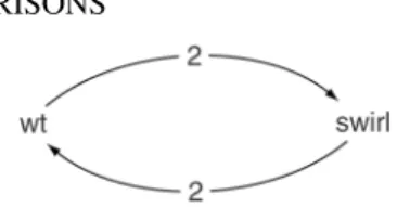
The results from the swirl zebrafish experiment were given to us by Katrin Wuennenberg-Stapleton from the Ngai Lab at University of California, Berkeley, while the swirl embryos themselves were generously provided by David Kimelman and David Raible from the University of Washington in Seattle. The experiment was carried out using zebrafish to study early development in vertebrates. Swirl is a point mutation in the BMP2 gene that causes defects in the organization of the developing embryo along its dorsal-ventral body axis. This results in a reduction of cells showing ventral cell fates (i.e., cell types that are normally formed only within the ventral aspect of the embryo), such as blood cells are reduced, whereas dorsal structures such as somites and notochord are expanded. A goal of this swirl experiment was to identify genes with altered expression in the swirl mutant compared to the wild-type zebrafish. The data are from four replicate slides: two sets of dye-swap pairs. For each of these slides, target cDNA from the swirl mutant was labeled using one of the Cy3 or Cy5 dyes and the target cDNA wild-type mutant is labeled using the other dye. Figure 2.3 is the graphical representation of this experiment.
In this case study, target cDNA was hybridized to microarrays containing 8848 cDNA probes. The microarrays were printed using4×4print-tips and are thus partitioned into a4×4grid matrix. Each grid consists of a22×24spot matrix that was printed with a single print-tip. In this and the other studies discussed next, we call the spotted
Figure 2.3 Case Study I: The swirl experiments provided by Katrin Wuennenberg-Stapleton from the Ngai Lab at the University of California, Berkeley. This experiment consists of two sets of dye swap experiments comparing gene expression between the mutant swirl and wild-type (wt) zebrafish. The number on the arrow represents the number of replicated experiments.
cDNA sequences “genes,’’ whether or not they are actual genes, ESTs (expressed sequence tags), or cDNA sequences from other sources.
Case Study II: Scavenger receptor BI mouse experiment
The scavenger receptor BI (SR-BI) experiment was carried out as part of a study of lipid metabolism and atherosclerosis susceptibility in mice, Callow et al. (2000). The SR-BI gene is known to play a pivotal role in high-density lipoprotein (HDL) metabolism. Transgenic mice with the SR-BI gene overexpressed have very low HDL cholesterol levels, and the goal of the experiment was to identify genes with altered expression in the livers of these mutant mice compared to “normal’’ FVB mice. The treatment group consisted of eight SR-BI transgenic mice, and the con-trol group consisted of eight normal FVB mice. For each of these 16 mice, target cDNA was obtained from mRNA by reverse transcription and labeled using the red-fluorescent dye Cy5. The reference sample used in all 16 hybridizations was prepared by pooling cDNA from the eight control mice and was labeled with the green-fluorescent dye Cy3. The design would have been better if the reference sam-ple had come from adifferentset of control mice. In this experiment, target cDNA was hybridized to microarrays containing 5548 cDNA probes, including 200 related to lipid metabolism. These microarrays were printed in a4×4matrix of sub-arrays, with each sub-array consisting of a19×21array of spots. The data are available
Figure 2.4 Case Study II: The SR–BI experiments provided by Matt Callow from the Lawrence Berkeley National Laboratory. This experiment consists of eight slides comparing gene expres-sion between the transgenic SR–BI mice and the pooled control (WT*). Another eight slides comparing gene expression between normal FVB (WT) mouse and pooled control. The number on the arrow represents the number of replicated experiments.
fromhttp://www.stat.Berkeley.EDU/users/terry/zarray/Html/
srb1data.html.
Single-slide methods
A number of methods have been suggested for the identification of differentially expressed genes in single-slide, two-color microarray experiments. In such experi-ments, the data for each gene (spot) consist of two fluorescence intensity measure-ments,(R, G), representing the expression level of the gene in the red (Cy5) and green (Cy3) labeled mRNA samples, respectively. (The most commonly used dyes are the cyanine dyes, Cy3 and Cy5, however, other dyes such as fluorescein and X-rhodamine may be used as well). We distinguish two main types of single-slide methods: those which are based solely on the value of the expression ratioR/Gand those that also take into account overall transcript abundance measured by the productRG. Early analyses of microarray data (DeRisi et al., 1996; Schena et al., 1995, 1996) relied on fold increase/decrease cutoffs to identify differentially expressed genes. For example, in their study of gene expression in the model plantArabidopsis thaliana, Schena et al. (1995) use spiked controls in the mRNA samples to normalize the signals for the two fluorescent dyes (fluorescein and lissamine) and declare a gene differentially expressed if its expression level differs by more than a factor of 5 in the two mRNA samples. DeRisi et al. (1996) identify differentially expressed genes using a±3cutoff for the log-ratios of the fluorescence intensities, standardized with respect to the mean and standard deviation of the log ratios for a panel of 90 “housekeeping’’ genes (i.e., genes believed not to be differentially expressed between the two cell types of interest).
More recent methods have been based on statistical modeling of the(R, G)pairs and differ mainly in the distributional assumptions they make for(R, G)in order to derive a rule for deciding whether a particular gene is differentially expressed. Chen et al. (1997) propose a data dependent rule for choosing cutoffs for the red and green intensity ratio R/G. The rule is based on a number of distributional assumptions for the intensities(R, G), including normality and constant coefficient of variation. Sapir and Churchill (2000) suggest identifying differentially expressed genes using posterior probabilities of change under a mixture model for the log expression ratio logR/G(after a type of background correction, the orthogonal residuals from the robust regression of logR versuslogG are essentially normalized log expression ratios). A limitation of these two methods is that they both ignore the information contained in the productRG. Recognizing this problem, Newton et al. (2001) con-sider a hierarchical model (Gamma–Gamma–Bernoulli model) for(R, G)and suggest identifying differentially expressed genes based on the posterior odds of change under this hierarchical model. The odds are functions ofR+GandRGand thus produce a rule which takes into account overall transcript abundance. The approach of Hughes et al. (2000b) (supplement) is based on assuming thatRandGare approximately independently and normally distributed, with variance depending on the mean. It thus also produces a rule which takes into account overall transcript abundance.
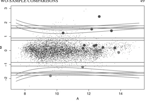
Figure 2.5 (See color insert following page xxx.) Single-slide methods: AnMA-plot showing the contours for the methods of Newton et al. (2001) (orange, odds of change of 1:1, 10:1, and 100:1), Chen et al. (1997) (purple, 95% and 99% “confidence’’), and Sapir and Churchill (2000) (cyan, 90%, 95%, and 99% posterior probability of differential expression). The points corresponding to genes with adjusted p-value less than 0.05 (based on data from 16 slides) are colored in green (negativet-statistic) and red (positivet-statistic). The data are from transgenic mouse 8.
As a result, each of these methods produces a model dependent rule which amounts to drawing two curves in the(logR,logG)-plane and calling a gene differentially expressed if its(logR,logG)-falls outside the region between the two curves. We apply Chen et al. (1997), Newton et al. (2001), and Churchill (2000)∗ single-slide methods to one slide from the SR–BI experiment. The different methods are used to identify genes with differential expression in mRNA samples from individual treat-ment mice compared to pooled mRNA samples from control mice. Using anMA-plot, Figure 2.5 displays the contours for the posterior odds of change in the Newton et al. (2001) method, the upper and lower limits of the Chen et al. (1997) 95% and 99% “confidence intervals’’ forM, and the contours for Sapir and Churchill’s 90%, 95%, and 99% posterior probabilities of differential expression. The regions between the contours for the Newton et al. (2001) method are wider for low and high intensities A, this being a property of the Gamma distribution which is used in the hierarchi-cal model. The genes identified as having differential expression between the SR–BI
∗Note that we are not performing the orthogonal regression for the log transformed intensities (Part I of the poster). The orthogonal residuals of Sapir and Churchill are essentially normalized log expression ratios. We have simply implemented Part II of the poster and are applying the mixture model to our already normalized log-ratios.
transgenic and the wild-type on the basis of all 16 slides (Callow et al., 2000) are highlighted in green (down-regulated) and red (up-regulated) in the figure. None of the methods satisfactorily identify all 13 genes found using all of the data on this slide, and the nature of their failure strongly suggests that these methods should not be relied upon in general. In our view, the statistical assumptions the different meth-ods make are just too strong, and inconsistent with the data, being unlikely to capture the systematic and random variability inherent these data. Furthermore, it is hard to see how a within-slide error model can capture between-slide variation, and error probabilities relating to detection of differentially expressed genes should relate to repeated hybridizations.
No single-slide or single-chip comparison exists for radiolabeled target hybridized to cDNA spots on nylon membranes or for high density short oligo arrays (i.e., for the single color systems). In order to compare mRNA from two cell populations in these cases, we need at least two nylon membranes or two chips, including at least one with target mRNA from each of the populations of interest. Assuming that we have exactly one membrane or chip from each of the cell samples, the problem becomes formally quite similar to the single-slide, two-color problem just discussed, though the details differ in important ways between nylon membranes and for high-density short oligo chips. With exactly two nylon membranes the situation really is quite similar to a single two-color slide, in that we have no more to go on that the two log intensities for each spot. Thus, determining differentially expressed genes can be no more than drawing lines in the associated plane, and the previous discussion applies, though not all the methods mentioned have been advocated in the nylon filter context. With high-density short oligo arrays, the situation is better. Approximately 11–20 probes for each gene or EST, and so there is information that permits us to estimate a standard error for each estimated log-ratio, or to carry out a significance test. Details of the Affymetrix methods for comparing two chips can be found at the following Web site:http://www.affymetrix.com/products/software/specific/ mas.affx. This approach works reasonably well in practice, though it is not clear that thep-values can be given their usual interpretation.
Replicate slides: design
Before considering methods for identifying differentially expressed genes involving replicate slides, let us briefly discuss the design question for the simple treatment-control comparison with two-color arrays.
Consider the two designs described in Figure 2.2. The goal of both designs is to compare two target samples T andC, and identify differentially expressed genes between them. Suppose that we plan on doing two hybridizations, and that quantity of RNA is not a limiting factor. For a typical gene on a slide, we denote the intensity value for the two target samples byT andC. Thelogbase 2 transformation of these values will be writtenlog2Tandlog2C, respectively, and when reference samplesR andRare used, we will writelog2Randlog2R. In addition, we denote the means of
the log-intensities across slides for a typical gene byα=Elog2Tandβ=Elog2C, respectively. Then, for the gene under study,φ=α−βis the parameter representing the differential expression between samplesT andC, which we want to estimate. The variances and covariances of the log-intensities for a typical gene across slides will be assumed to be the same for all samples, that is, we suppose that differential gene expression is exhibited only through mean expression levels, and we always view this on the log scale. In addition, we assume for the moment that the replicate measurements on different slides are independent. For any particular gene, let us assume thatσ2is associated with the variance for one such measurement. (This may vary from gene to gene.) It follows that thedirectestimate of the differential expression and its corresponding variance are:
ˆ
φD=12(log2(T/C) + log2(T/C))andvar( ˆφD) =σ2/2
respectively. Alternatively, if we make use of a common referenceRsay, then from our two hybridizations, theindirectestimate of log-ratio and its variance are:
ˆ
φI = log2(T/R)−log2(C/R)andvar( ˆφI) = 2σ2
The resulting relative efficiency of the indirect versus the direct design for estimating α−βis thus4. This is the key difference between direct and indirect comparisons, and the reason why we recommend under many circumstances that direct comparisons are to be preferred. The factor 4 depends critically on our independence assumption, but we will see shortly that under very general assumptions, the direct comparison is never less precise than the indirect one.
Replicate slides: direct comparisons
A number of approaches can be used here, and we briefly discuss each of them.
Classical
Suppose that we havenreplicate hybridizations between mRNA samplesAandB. For each gene, we can compute the averageM¯ and the associated variances2of the nlog-ratiosM = log2A/B. In line with the early work summarized above, it would be natural to identify differentially expressed genes by taking those whose values|M¯| exceed some threshold, perhaps one determined by the spread ofM¯ values observed in related self-self hybridizations. It would be equally natural to statisticians to calculate thet-statistict=√nM/s, and make decisions on differential expression on the basis¯ of|t|. Both strategies are reasonable, the first implicitly assigning equal variability to every gene, the second explicitly permitting gene-specific variances across slides; however, neither strategy is entirely satisfactory on its own. Large values ofM¯ can be driven by outliers, as the value ofnis typically quite small (in our experience ≈2−8), and the technology is quite noisy. On the other hand, with tens of thousands of|t|statistics, it is always the case that some are quite large in comparison with
the others because their denominatorssare very small, even though their numerators √
n|M¯|may also be quite small, perhaps almost zero.
Empirical Bayes
Several more or less equivalent solutions are available to the problem of very small variances giving rise to larget-statistics, ones which lead to a compromise between solely usingtand solely usingM¯. One solution is to discount genes with a smallM¯ whose standard errors are in the bottom 1%, for example. This leaves open the choice of cutoffs onM¯ and the standard error. More sophisticated solutions in effect stan-dardizesM¯ by something midway between a common and a gene-specific standard error. For example, Efron et al. (2000) slightly tune thet-statistic by adding a suitable constant to each standard deviation, using
t∗= √nM¯ a+s
One choice forais the 90th percentile of standard deviations, while another mini-mizes the coefficient of variation (see Efron et al., 2000; Tusher et al., 2001). This solution recalls the empirical Bayes (EB) approach to inference, which is natural in the microarray context where thousands of genes exist. A more explicitly EB approach, which is almost equivalent to the preceding one, apart from the choice ofa, is pre-sented in L¨onnstedt and Speed (2001); we illustrate it next. In addition to these two just cited, there are other EB formulations of the problem of identifying differentially expressed genes (see e.g., Efron et al., 2001; Long et al., 2001; Baldi and Long, 2001). In L¨onnstedt and Speed (2001), data from all the genes in a replicate set of experiments are combined into estimates of parameters of a prior distribution. These parameter estimates are then combined at the gene level with means and standard deviations to form a statisticB,which is a Bayes log posterior odds for differential expression.B can then be used to determine if differential expression has occurred. It avoids the problems of the average M and thet-statistic just mentioned. In the same article, a comparison is conducted between the B-statistic, the previous statistics t∗, and truncation of small standard errors. The differences are not great.
Note that the preceding analysis, and others like it, treatsM values from different genes as conditionally independent, given the shared parameters, which is very far from the case, although it may not matter much at this point. Any attempt to provide a semiformal analysis of replicated log-ratios may require this assumption, or something very similar to it. By contrast, the permutation-based analyses described next do not require this assumption, but they do not apply here.
Robustness
The EB solution to the problems outlined in the classical approach focus on smooth-ing the empirical variances of the genes, thereby avoidsmooth-ing the situation where tiny variances can create large t-statistics. A different approach is to replace M¯ in the
numerator, in effect avoiding the problems which result from outliers coupled with small sample sizes. The obvious solution is to use a robust method of estimation of the parameterφwherever possible (Huber, 1981; Hampel et al., 1986; Marazzi, 1993). Alternatively, use could be made of a nonparametric testing procedure, for example one based on ranks. The problem here is that the sample sizes are small, not infrequently as low as two or three.
Let us note in passing that the use of robust estimates of location with sample sizes as small as two or three is not without its problems. In such cases, estimates of standard errors can hardly be relied upon, and instability in the associated “t-statistics’’ is not uncommon. Users of standard robust procedures such asrlmin R and SPlus should take care and not simply rely upon default parameter settings in the algorithms. It is to be hoped that the greatly increased use of robust methods stimulated by microarray data will lead to further research on this topic.
Mixture models
Many approaches to identifying differentially expressed genes in this context use mixture models, including the EB ones just discussed. Lee et al. (2000) use a two-component normal mixture model for log-ratios in two-color arrays, one two-component for differentially expressed genes and another for the remainder of the genes. They estimate the parameters of their model by maximum likelihood and compute posterior probabilities using the estimated parameters. In a sense, this is another EB model, but not one with gene-specific variances, and so quite different in character from those discussed previously. Efron et al. (2001) also have a two-component mixture model, but it is for Affymetrix GeneChip data, and it is more general that the previous one. Their mixture model is for the statistict∗instead of for log-ratios, and they make no parametric assumptions about their mixture components. More recently, Pan (2002) discussed a multicomponent normal mixture model, extending the of analysis of Lee et al. (2000) toward that of Efron et al. (2001).
Fixed and random effects linear models
One approach to the analysis of two-color microarray data and the determination of differentially expressed genes makes use of linear models and the analysis of variance (Kerr et al., 2001; Wolfinger et al., 2001; Jin et al., 2001). These authors model un-normalized log intensities with linear models which include terms for slide, dye, gene and treatment, a subset of the interactions between these effects, and a random error term. Important differences exist between the approaches of Kerr et al. (2001) and the other two papers in the way in which normalization is incorporated, in whether terms are fixed or random, and in assumptions about the error variances. We illustrate the approach of Kerr et al. (2001) next, and we begin by presenting their model for our Case Study I. We label array effects (A) byi, dye effects (D) byj, treatment effects (V) bykand gene effects (G) byg. Their model for the log of the intensityyijkgis:
wherei= 1, . . . ,4,j= 1,2,k= 1,2, andg= 1, . . . ,8848. In Case Study I, which consists of a two sample comparision, the treatment effectVk represents the mutant (V2) or wild-type (V1) samples. In this model, all terms are fixed apart from the random error terms. The term of interest here is(V G)kg and the value(V G)2g−(V G)1g estimates the level of differential expression between the mutant and the wild type samples for gene g. This model can easily be extended to cover multiple samples and factorial designs, although we do it differently in the section 3 on “Linear model analyses’’. Further discussion of fixed and random effects linear model is given there.
Error models
Several groups have used more fully developed error models for measurements on microarrays, and sought to identify differentially expressed genes by making use of their error model. These include Roberts et al. (2000), Ideker et al. (2000), Rocke and Durbin (2001), Theilhaber et al. (2001), and Baggerly et al. (2001). Ideker et al. (2000) has made their software publicly available, so we illustrate this approach in Case Study I. Their error model is for pairsT andCof unnormalized un-logged intensities for the same spot, namely,
T = µT +µT+δ
C = µC+µC+δ
where (, )and (δ, δ)are independently bivariate normally distributed across spots with means(0,0)and separate, general covariance matrices that are common to all spots on the array. Thus, six parameters exist for the error model, in addition to parameters determining the expected values. This model is close, but not quite identical to a similar model for(logT,logC), one that permits the two components to be correlated, with a correlation which is common to all the spots. Intensities from distinct spots on the same slide, or spots on different slides are taken to be independent. Roberts et al. (2000) and Rocke and Durbin (2001) use a similar model, but do not allow the different channel intensities to be correlated.
In order to identify differentially expressed genes, Ideker et al. (2000) fit the model to two or more slides by maximum likelihood. Differential expression is then determined by carrying out a likelihood ratio test of the null hypothesisµT =µCfor each gene separately, resulting in a likelihood ratio test statisticλfor each gene.
Other approaches
Working with Affymetrix GeneChip data, Thomas et al. (2001) use a variant on the simple two-samplet-statistic which starts from a nonlinear model including sample-specific additive and multiplicative terms. In the same GeneChip context, Theilhaber et al. (2001) present a fully Bayesian analysis, building on a detailed error model for such data. We refer readers to these articles for further details.
Replicate slides: indirect comparisons
When the comparisons of log-ratios in a two-color experiment are all indirect, the procedures just described need to be modified slightly. Typically, we would have some number,nT, of slides on which the gene expression of sampleTis compared to that of a reference sampleR, leading tonT log-ratiosM = log2T/R, and a similar set ofnC log-ratios log2C/R from sampleC. The analogues of the average and t-statistics here are the differences between the meansM¯T−M¯Cand the two-sample
t-statistic is
t= M¯T −M¯C sp1/nT + 1/nC
wherespis the pooled standard deviation.
The problems with these two statistics are completely analogous to those described in the previous section withM¯ andt, and the solutions are similar: modifyspor use robust variants ofM¯T −M¯Candt.
We note in closing this brief review that some non-statisticians addressing these two-sample problems in the microarray literature have devised novel approaches. Galitski et al. (1999) and Golub et al. (1999) sought to identify single differentially expressed genes by computing for each gene the correlation of its expression profile with a reference expression profile, such as a vector of indicators for class membership. In the case of two classes, this correlation coefficient is a type oft-statistic. Genes were then ranked according to their correlation coefficients, with a cutoff derived from a permutation distribution.
Illustrations using our case studies
We now describe the results of applying some of the methods just discussed to Case Studies I and II. It should be understood that we are not attempting to present thorough analyses of these data sets, in part because of lack of space, and in part because more effort always goes into the determination of differential expression than the application of a single statistical analysis. Nevertheless, we hope that what follows gives an indication of the potential of the methods we illustrate. We have certainly found them useful in similar contexts, particularly the graphical displays.
Plots: averages, SDs,t-statistics and overall expression levels
Important features of the genes which might be differentially expressed can be found by examining plots oft-statistics, their numeratorsM¯ and denominatorss, and the corresponding overall expression levels. The overall expression level for a particular gene is conveniently measured by the quantityA, the average of¯ A= log2√RGover all the slides in the experiment.
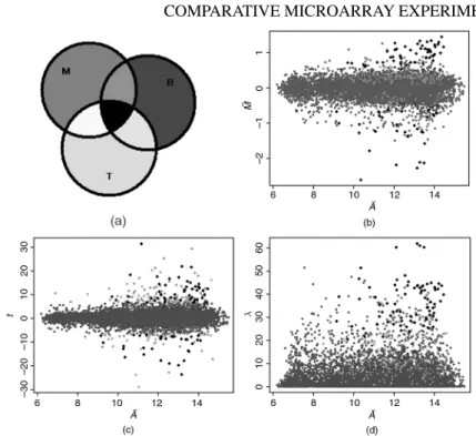
Figure 2.6 (See color insert following page xxx.) Graphical illustration of Case Study I: swirl experiment. (a) The color code that defines three groups of 250 genes consisting of largest values of|M|¯ ,|t|andBvalues; (b)M¯A¯-plot; (c)tvs.A¯; (d)λvs.A.¯
Let us begin with theswirlexperiment. In Figure 2.6b, 2.6c and 2.6d we have plotted the average log ratioM¯, thet-statistic and the log-likelihood ratio statisticλfrom Ideker et al. (2000) againstA. We began by defining three groups of 250 spots each,¯ being those having the largest values of|M¯|,|t|andB, respectively, and then plotted the points according to the color code depicted in Figure 2.6a. Thus, points corre-sponding to spots in all three groups are colored heavy black, while the very light black spots, the overwhelming majority, are in none of the groups. Clearly, the heavy black spots are the main candidates for differential expression. Spots belonging to large|t|group only are green, while those in the large|M¯|and largeBand not large |t|groups are pink. The absence of points colored yellow is noteworthy: any spots with large|t|and large|M¯|already have largeB. This is not uncommon, and shows thatBis, in general, a useful compromise betweentandM¯.
It is clear from these plots, and is not infrequently the case, that some points are well separated from the cloud. The genes corresponding to these points are likely to be differentially expressed, and we recommend this informal approach identifying such genes. In many cases, this evidence is as solid as any we are able to obtain for differential expression. Note the broad agreement on the black points in all three of the panels. Figure 2.7a shows the nature ofBrather clearly, while Figure 2.7b shows the role of the standard deviation (SD) in determining whether a givenM¯ ends up
Figure 2.7 (See color insert following page xxx.) Case Study I: swirl experiment. Plots of (a) Log oddsBvs.M¯ and (b)tvs.log2(SD). Spots (genes) corresponding to large|M¯|,|t|and Bvalues highlighted according to color code shown in Figure 2.6a.
having a large|t|as well, with it being clear how largeBrelated to the other two. The green points are those with smaller SDs, in comparison with the solid black, pink, and light blue spots. Of course, much of this is dependent on the cutoffs defining our groups, which were determined after looking at the plots, but the message of these plots is general.
Turning to the SR–BI experiment, Figure 2.8a shows a plot ofM¯T −M¯CagainstA¯, while Figure 2.8b showstagainstA¯. Here, we have given no analogue ofB, though one could be developed. In this case it is the yellow spots that should attract our attention, and it should be clear that our choice here of 250 in the two groups is too large. Looking at Figure 2.9a and 2.9b, we see that in general a large|M¯T −M¯C|is more likely to go with a large|t|if the SD is not too large and not too small, which
Figure 2.8 (See color insert following page xxx.) Case Study II: SR-BI experiment: (a)M¯A¯ -plot; (b)tvs.A.¯ Spots (genes) corresponding to large|M¯|and|t|values highlighted according to color code shown in Figure 2.6a.
Figure 2.9 (See color insert following page xxx.) Case Study II: SR–BI experiment. (a)tvs.
log2(SD); (b)log2(SD)vs.A¯
is roughly equivalent to having anA¯value that is not too small and not among the largest ones. We see clearly from Figure 2.9b that largerA¯values go with smaller values of the SD, and we remark that many plots of this kind would show a much greater increase in SD for lower values ofA. That is often quite evident in the¯ M¯A-¯ plot (Figure 2.8a) as a ballooning in the low intensity ranges, a phenomenon we have prevented by using a smaller and less variable background adjustment (see Yang et al., 2002a).
How would we use these statistics to identify differentially expressed genes? It is tempting to answer in the following way: Simply rank the genes on the basis of|M¯|,t orB, and determine a cutoff in some sensible way. This is in effect what we have done in producing the plots, without being careful about cutoffs; however, the plots also tell us that a ranking based on just one of these statistics is not necessarily the best we can do. The reason is this: A spot’s overall intensity valueA¯can be a useful indicator of the importance that can be attached to itsM¯,t, orBvalue. Typically, considerably fewer genes exist with largeA¯values, and a spot can stand out from the cloud in the larger
¯
Arange with a smallerM¯,t, orBvalue than than would be necessary to stand out in the lowA¯region. At times, the difference can be striking, although this is not the case with our illustrative examples. Most methods of identifying differentially expressed genes in the present context do not make explicit use of the overall intensity or any related values, although approaches using fully specified error models in effect do so. One problem with full error models is that they invariably assume that observations on different slides are independent, which can be very far from the case, and this vitiates their exact probability calculations.
In summary, we regard the determination of differentially expressed genes on the basis of a small number of replicates as a problem for which more research is needed. It is clear that the values ofM¯,t,B(or their analogues) are highly relevant, but the values ofA¯and the SD should not be ignored. For the present moment, we feel that determining cutoffs is best done informally, following visual inspection of plots like the ones we have shown. Naturally, scientific considerations such as the expected
number of differentially expressed genes and the number of follow-up experiments that might be feasible, are also relevant in determining cutoffs, and we feel thatA¯ should also play a role.
Ranking genes by sets of statistics
Whether we use of|M¯|,|t|,B,λor some similar statistic to provide a ranking of genes corresponding to the strength of evidence of differential expression, it is intuitively clear that our preferred genes should rank highly on all these criteria. Hero and Fleury (2002) describe a valuable method of selecting genes which are highly ranked in a suitable multidimensional sense. They describe what they termPareto fronts in
multicriterion scattergrams, which are points that are maximal in the componentwise ordering (Pareto optimal) in theP-dimensional scatterplots of a desired set of P criteria. As well as giving some modified versions of Pareto optimal genes, they demonstrate that their ideas are applicable to a wide range of gene filtering tasks, not just that of detecting differentially expressed genes. We refer to the paper Hero and Fleury (2002) and also Fleury et al. (2002b) for a fuller discussion of the method.
Assessing significance
After ranking the genes based on a statistic, a natural next step is to choose suitable cutoff values defining the genes that might be considered as significant or differentially expressed. In this section, we consider the extent to which this can be done informally. We focus on two types of plots.
Quantile–quantile plots
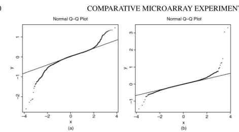
A simple graphical approach is to examine theQuantile–Quantile plots(Q–Q plots) for certain statistics. Q–Q plots are a useful way to display theM¯ ort-statistics for the thousands of genes being studied in a typical microarray experiment. The standard normal distribution is the natural reference, and the more replicates that enter into an average ort-like statistic, the more we can expect the majority of the statistics to look like a sample from a normal distribution. With just four replicates, which is equivalently eight log intensities entering into our averages, we cannot expect and do not get a very straight line against he standard normal; however, the plot can have value in indicating the extent to which the extremet-statistics diverge from the majority. Q–Q plots informally correct for the large number of comparisons, and the points which deviate markedly from an otherwise linear relationship are likely to correspond to those genes whose expression levels differ between the two groups. At times, we can tell where the outliers end and the bulk of the statistics begin (see e.g., Dudoit et al. (2001b), but unfortunately this is not the case with either of the present examples.
Figure 2.10 Quantile-quantile (Q–Q) plot for (a) one-samplet-statistics from the swirl exper-iment; (b) two-samplet-statistics from the SR–BI experiment.
Figure 2.10a is typical of many Q–Q plots which are not very helpful. The tails of the distrubutions of theset-statistics are far from those of a normal (ort) distribtion. The best we can hope for in such cases is that some points are obviously outliers with respect to the nonnormal distribution, and this is true to some extent here, especially for large negativets.
The picture in Figure 2.10b is clearer. This is for the SR–BI experiment, and is perhaps what we would expect, as there are 16 observations in each of theset-statistics. We see about a dozen genes with “unusual’’t-statistics, and these are obviously good can-didates for genes exhibiting differential expression (both up and down-regulation). Some of these genes were verified to have the observed behaviour in follow-up exper-iments.
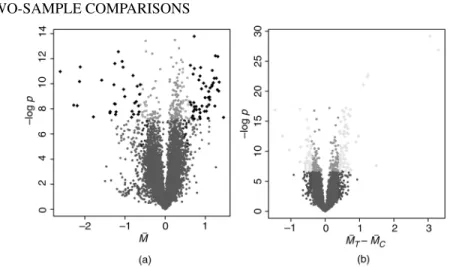
p-value vs. average M (volcano) plot
Another plot which allows outliers to reveal themselves among thousands of statistics is the so-called volcano plot (Wolfinger et al., 2001), Figure 2.11. We have already seen one plot like this in Figure 2.7a, where the log-odds corresponding to a given value of the statisticBwas plotted againstM¯. More commonly, people plot the logs of raw (i.e., model-based, unadjusted)p-values against the estimated fold change on a log scale,M¯ (Wolfinger et al., 2001). Whether thep-values are calculated assuming a tor a normal distribution is not so important here. The color code indicates how these plots capture some aspects of the plots we presented earlier in what is perhaps a more convenient form; see especially the solid black points in Figure 2.11a and the yellow points in Figure 2.11b.
So far, the approaches we have offered for identifying differential expression are all informal. In many cases, this will be adequate. The number of genes that are selected as possibly differentially expressed will in general depend on many things: the aims