Interactive Physically-Based Cloud Simulation
Derek Overby
[email protected]
Zeki Melek
[email protected]
Texas A&M University
College Station, TX
John Keyser
[email protected]
Abstract
Artificial clouds play an important role in the computer generation of natural outdoor scenes. Realistic modeling and rendering of such scenes is important for applications in games, military training simulations, flight simulations, and even in the creation of digital artistic media. We pro-pose a model for simulating cloud formation based on an efficient computational fluid solver. We combine the fluid solver with a model of the natural processes of cloud for-mation, including buoyancy, relative humidity, and conden-sation. This allows us to simulate the formation and growth of clouds at interactive rates.
1
Introduction
In order to produce visually pleasing artificial clouds, we must have both efficient methods for visualizing vol-ume data and useful interactive applications for generating this data. The visualization of volumetric data has been one of the larger challenges that the graphics community has addressed in the last few decades. As we have learned to improve our methods of visualization, we must also strive to improve our methods for generation. In this paper, we fo-cus on the simulation of physical processes that contribute to the formation of clouds in our atmosphere1. By simulat-ing these physical processes we are able to more accurately model the structure of a cloud that forms under given atmo-spheric conditions.
Traditionally, cloud structure has been generated by ei-ther procedural or fractal methods[12]. While these meth-ods may at times produce visually compelling results when coupled with complex rendering techniques, these struc-tures are essentially random and are difficult to modify or 1In this paper, when we refer to the atmosphere, we are referring specif-ically to the troposphere or sphere of weather[21]. The troposphere is the lowest division of our atmosphere which extends from the ground to ap-proximately 12km, and is where most visible cloud formations occur.
control interactively for creating different cloud types. Our method allows the user to interact with a physically-based simulated environment in order to produce the desired cloud formation. All the user needs is a basic understanding of the fundamental processes involved in cloud formation: buoy-ancy, relative humidity, and condensation.
The software model we have presented in this paper rep-resents a new approach to explicitly modeling the many natural processes that lead to atmospheric cloud formation using an interactive numerical fluid simulator. Also, our model is one of few to date which has addressed more than one type of cloud.
In this paper, we first discuss prior work on modeling clouds and fluid motion. We then discuss the model we use to simulate cloud formation, including the necessary modi-fications to the fluid solver. We describe the implementation we have created, including how it can be used to create var-ious cloud types. Finally we discuss how our results can be incorporated into various rendering systems.
2
Background Material
Cloud modeling has been a focus of prior research in computer graphics. Researchers have been active in devel-oping methods for simulating, visualizing, and predicting clouds and other natural phenomena that occur in our atmo-sphere, as well as methods for simulating the fluid motion that occurs in the atmosphere. Cloud modeling is also an area of research in meteorology, however most of the mod-els developed in this field are designed for simulation at a larger scale, are geared toward predictive accuracy rather than visual quality, and are not designed for interactive sim-ulation. While our model is physically-based, we do not at-tempt to create a model of the scale and accuracy achieved by meteorological simulators. In section 2.1 we discuss pre-vious models of cloud formation in computer graphics and some of the advantages and shortcomings of these methods. In section 2.2 we summarize the basic principles involved in the physical process of cloud formation. We then present
a brief introduction to the fluid model we will be using for our simulation in section 2.3.
2.1
Cloud Models in Computer Graphics
Within the field of Computer Graphics there has been extensive research aimed at generating realistic looking clouds. While most of this research has been aimed at de-veloping advanced methods for rendering clouds and other fuzzy objects, there has also been considerable research into generating the volumetric structure of such objects. In sec-tion 2.1.1 we discuss previous models of cloud structure, and in section 2.1.2 we discuss various rendering methods that have been used for clouds.
2.1.1 Structural Models
Some of the earliest cloud models were based on random generation of structures by procedural functions. These include methods presented by Gardner[5], Perlin[15] and Lewis[10]. The problem with such methods is that in the quest to mimic the shape of natural clouds, they can quickly become gross mathematical abstractions of simple fluid mo-tion. The benefit to using such methods, however, lies in the scalability of fractal based methods. These methods can be used to generate infinitely small detail, which is highly desirable in cloud models. (In our model, generating such detail will be left to rendering methods.)
In their 1992 paper, Nagle and Raschke[12] presented a model of cloud growth based on a simple Boolean func-tion iterated within a volumetric data space. These cellu-lar automaton-based methods can give a somewhat realis-tic looking growth pattern for the formation of a cloud, but these methods are difficult to modify interactively. Another approach to modeling cloud formation has been presented by Neyret[13]. This model can be used to generate a surface representation of convective cloud formations, using evolv-ing bubbles and turrets as well as other simple abstractions of complex fluid interactions. A shortcoming of this model is the lack of interior detail for the generated cloud struc-tures. Ebert has also developed a unique cloud modeling method based on deforming implicitly defined primitives over time[3].
Our approach follows that of other, more physically-based approaches. This includes the work of Kajiya and Von Herzen[8] and Miyazaki et al.[11]. However, Kajiya’s model does not account for variation in pressure within the atmosphere and accounts for viscous effects, which are neg-ligible for a standard atmospheric application2. He also uses
a different approach to modeling and solving for the spatial effects of atmospheric fluid dynamics. Miyazaki’s model, which is based on an earlier model by Dobashi et al.[2],
2This will be shown later in section 2.3.
uses a coupled map lattice (rather than a more general fluid solver), developed by Kaneko[9] to simulate the physical process of cloud formation.
2.1.2 Rendering Models
Computer rendered clouds are often generated for the pur-pose of background imagery, and therefore the primary goal of the modeler is to “fool” the eye into dismissing the puffy thing it sees in the background as a cloud. By making the cloud appear more natural in color and texture, the artist can draw the viewer’s eye away from the actual structure of the cloud and toward the heart of the image. Such effects may be achieved using rendering techniques and artistic con-trol, without actually putting much effort into the underly-ing model of the cloud. Much of the research in computer-generated clouds has tended to focus more on bringing re-alism to clouds through the art of rendering.
Some of the earliest work included that of Kajiya and von Herzen[8], who used multiple scattering to render high-albedo volume data. Others have generated volumetric ren-derings based on other physical simulations (e.g. Stam[18]). For rendering clouds, the incorporation of single and multi-ple scattering by Nishita et al.[14] and atmospheric attenu-ation by Dobashi et al.[2] have produced some of the most effective recent renderings. These methods often make use of imposters, or billboards, to speed up the rendering pro-cess.
Recent research into interactive rendering methods in-cludes that by Harris and Lastra[6]. Their paper focuses on using imposters to speed up rendering, approximating multiple forward and anisotropic scattering of light through volumetric data. While this method succeeds at achieving excellent frame rates when rendering particle-based cloud structures, currently this method is best suited for rendering static clouds, but not dynamic, evolving clouds.
2.2
Physical Process
Our model of cloud formation is physically-based. We simulate the condensation of water vapor within the atmo-sphere based on physical parameters such as relative hu-midity and buoyancy. We will give a brief description of the physical process of atmospheric cloud formation.
The first requirement for cloud formation to occur is the presence of “dirty moist air.” Aside from having air that contains humidity (water vapor), we must also have air that contains tiny particles, called hygroscopic nuclei, upon which the water vapor can condense3.
The second requirement for clouds to form is the pres-ence of ascending air. This is most often caused in our atmosphere by thermal currents, which are the result of
buoyancy caused by temperature variations within our at-mosphere. As air near the surface of the earth is heated, it’s temperature increases. This causes the air to expand due to increased local pressure and then rise due to a decrease in density. Note that in our model we do not explicitly repsent this change in density but instead simulate only the re-sulting buoyant force based on the temperature difference. Ascension of air can also be caused by orographic uplift which is when air is ‘pushed up’ by the terrain below it. For example, clouds often form around mountain ranges as the air blows up and over the surface of the mountain[21].
As air rises, pushed by either buoyancy or orographic up-lift, the air expands as the pressure decreases. This causes the air to cool. Cool air is able to hold less water vapor than warm air, resulting in an increase in relative humidity4as a
moist air parcel rises. Eventually, the rising air will reach a point of saturation. The temperature at which this occurs is called the dew point. Once the dew point has been reached and if hygroscopic nuclei are present, condensation will oc-cur. This is not the end of the process, however, as conden-sation is an exothermic process, causing the release of latent heat of condensation. The transfer of energy increases the temperature of the nearby air, thus creating more buoyancy and increasing vertical velocity. This is why so many clouds seem to grow upward, especially when the surrounding air is calm. Different atmospheric conditions contribute to the growth of different cloud types, which will be discussed in section 4.
2.3
Fluid Models
Simulation of fluid flow has long been an active research area, with many applications. Early research was hindered by the large memory and processing requirements inherent when storing and manipulating volumetric data on a coarse grid. Recent research, however, has resulted in a method for producing visually realistic fluid motion on coarse 3D grids at interactive rates.
The Navier-Stokes equations describe the flow of a fluid. The solution is an approximation of incompressible flow. Incompressible flow contains no sharp changes in density, which are most often caused by supersonic shockwaves. This model is preferred to those of compressible flow be-cause compressible flow solutions require relatively small time steps to maintain accuracy and thus are more expen-sive to compute. In most situations incompressible flow models do not experience significant loss of accuracy, as long as the maximum flow speed remains below the speed of sound[7]5. The details of the Navier-Stokes equations are 4Relative humidity is the amount of water within a differential volume of air over the total amount of water vapor that differential volume can hold at saturation[21].
5The effects of supersonic shockwaves would require the use of a model of compressible fluid flow.
described in Appendix A.
The fluid solver we use for our simulation, presented by Stam[18], is based on this Navier-Stokes system. This method solves the Navier-Stokes fluid equations over a coarse grid. At each simulation step, the Navier-Stokes equations, neglecting the viscous term, are solved for each voxel in the grid. One of the main aspects of this method is the use of backward-tracing particle motion within the sys-tem. This approach allows for increased stability even when using large time steps (although taking larger time steps will always decrease numerical accuracy). For more details con-cerning implementation of the basic fluid solver, the reader should consult Fedkiw’s paper[4] or Stam’s paper[18] .
3
Software Model
In this section we discuss our proposed software model for the physical process of atmospheric cloud formation. In section 3.1 we discuss the basic atmospheric model that ac-counts for convective currents caused by variations in tem-perature, as well as condensation and the release of latent heat. In section 3.2 we discuss some modifications we have added to our fluid model to more accurately model the phys-ical atmosphere, and in section 3.3 we discuss the interface we have implemented for our software application.
3.1
Basic Atmospheric Model
In order to model the physical process of cloud forma-tion, we must first model the fluid flow of air within our atmosphere. Atmospheric air flow is based on a number of environmental factors, including large-scale wind motion and buoyancy of air due to local temperature differences.
In order to model the local motion of the air, we must model the thermal currents that occur in the atmosphere. However, instead of explicitly modeling temperature values at each grid point, we model the amount of heat energy in the system and let the temperature be solved for implicitly. This allows our system to more easily account for adiabatic cooling of rising air caused by decreasing pressure6. We are
able to compute the temperature of any point in the field by multiplying the amount of heat energy present by the pres-sure, shown in equation 1. This equation gives us the effect of an air parcel decreasing in temperature as it rises and ex-periences a decrease in pressure. The constant in equation 1 can be used to set the maximum temperature desired for the system.
(1) 6It should be noted that this concept is very similar to the notion of virtual temperature used earlier by Kajiya[8].
Figure 1. Heat enters the environment from defined sources, represented by spheres at the bottom. This creates buoyancy which causes convection currents within our sys-tem. The colored region shows the heat dis-tribution.
The pressure in our system is defined based on altitude. The pressure is 1.0 Bar at ground level and decreases expo-nentially with height to 0.1 Bar at the tropopause7. These values are taken directly from measurements within our own atmosphere[21].
Once we compute the temperature at each point we use this information to compute our buoyant forces. At each point, if the surrounding temperature is less than the current temperature at that point then we add a positive buoyant force. Likewise, if the surrounding temperature is greater than the current temperature, we add a negative buoyant force as shown in equation 2, where !#"%$'&)(+*-,.& is an
ap-propriate constant. This enables us to model the thermal currents in our atmosphere caused by temperature varia-tions. Note that, in contrast to some other methods, we do not explicitly define the convection currents; they are produced automatically as a result of modeling the heat dis-tribution and the resulting buoyancy. Figure 1 shows heat being added to the system and causing buoyancy, and figure 2 shows humidity within the system being advected upward by that buoyant force.
/
!#"%$'&)(+*-,.&10 2!#"%$'&)(+*-,.&436578$,(89:7;"<<$'"*-=>*%?%@ (2)
Next we compute relative humidity at each point. In fact, there are a number of measurements of humidity that can be used. These include relative humidity, specific humidity, mixing ratio, and absolute humidity[21]. In our model, we have chosen to compute relative humidity, which is given as the amount of water vapor contained within the air divided by the total amount of water vapor that could be held at saturation. The amount of water vapor the current volume can hold at saturation is directly proportional to the pres-sure, as shown in equation 4. This gives the desired effect of increasing relative humidity as pressure decreases.
7The tropopause refers to the upper boundary of the troposphere.
Figure 2. Humidity is shown being advected upward by thermal currents. The humidity is colored based on temperature, blue being cold and red being hot.
ACB 0 DFEHGG%IJLKM (NO<+P('Q$'< RTSUKEHG%SUKVWJXM (NO<+P('Q$'< (3) RTSUKEHG%SUKVWJXM (NO<+PX('Q$'<Y0[Z8$,(83 2\](N"<(N>^$'* (4)
Next we model condensation. We have already stated that the relative humidity at a given voxel must be at or near saturation for condensation to occur. If the concentration of hygroscopic nuclei is very high (above 0.75), condensa-tion can occur at lower relative humidity levels[21]. The amount of condensation at any point is a function of the rel-ative humidity and the concentration of hygroscopic nuclei, as shown in equation 5, where _,$'*-=+O*-;`O`= is a constant.
Be-cause of this relationship we can use the hygroscopic nuclei concentration to increase the probability of cloud formation in certain areas of our workspace, or likewise prohibit for-mation in other areas.
a ,$'*-=+O*-;`O`=C0 ACB 3 Bcb 3 2,$'*-=+O*-;`O`= (5)
Finally we compute the latent heat released from the phase transition of the water vapor. The amount of latent heat released is directly proportional to the mass of water vapor condensed. Therefore we can compute the amount of latent heat released as shown in equation 6. The constant
8(NO*%N will directly affect how quickly the simulated cloud
formation will grow upward when condensation begins.
d
8(NO*%N0
a
,$'*-=+O*-;`O`=43 8(NO*%N (6)
Note that altough there are many constant in equations 1–6, most of the constants are known physical values (e.g.
8(NO*%N is given asegfh13cij-kYl
m
? for water vapor at j]n
D
and 1.0
SUKo
, [20]). Although a user may change the constants to modify the results, doing so makes the simualation less realistic.
3.1.1 Incorporating into the Fluid Solver
We have discussed how we compute the parameters nec-essary to model the physical process of atmospheric cloud formation. We will now describe how we incorporate these computations into our fluid solver to create our model. The pseudocode contained in Appendix B should also help ex-plain how to implement our method.
Several data fields are maintained over a 3D grid. At each grid point the velocity, humidity (amount of water va-por), heat, and condensed water is stored. These fields are input into the fluid solver. The fluid solver advects the ve-locity field on itself, thus simulating fluid flow and updating the velocity values. In addition, the other data fields (the “density fields”) are advected based on the velocity, and al-lowed to diffuse and dissipate slightly (the actual amounts of diffusion and dissipation can be adjusted). We modify this process slightly as described below (section 3.2). At each time step, the fluid solver returns velocities in the x, y, and z directions as well as density values for each field (humidity, heat, and condensation) for each grid point.
After each time step, we compute the relative humidity at each voxel as described in equation 3. If the computed relative humidity is above a user-specified threshold and hy-groscopic nuclei are present, we then compute the amount of water vapor that will be condensed as given in equation 5. This value is first subtracted from the humidity field and then added to the condensation field. We then compute the amount of latent heat released as shown in equation 6, and add this amount to the heat field.
Based on the new temperatures, we compute buoyancy forces in the system. In addition, we add any external forces provided by wind. These forces modify the velocity field, and the simulation process is then repeated.
3.2
Modifications to the Fluid Solver
The fluid solver, for computational ease, assumes that pressure is constant in the system, which is certainly un-true over the atmospheric scale. In order to make the fluid model account for the variation in atmospheric pressure in the vertical dimension, we make two low-level modifica-tions to our solver. Specifically, we modify the velocity field at each step to account for the expansion of rising air and the conservation of momentum. Although these effects tend to be minor (velocities in our typical simulation are modified by less than 5%), the effects are not negligible over the scale of the simulation. While the resulting mo-tion is not a completely accurate model of fluid flow in the atmosphere, it does capture the primary differences from a constant-pressure simulation.
3.2.1 Expansion
The first addition accounts for the expansion of air as it in-creases in altitude. Air at lower altitudes is under more pres-sure and thus is more dense; as a parcel of air rises into a lower pressure region, it expands. We account for expansion of rising air as shown in a 2D example in figure 3. At each time step, for all positive vertical motion we add a propor-tional amount of horizontal motion in each direction. The net effect of this will be a horizontal expansive force along the boundary of any parcel moving upward. The amount of force added is proportional to the decrease in pressure expe-rienced over the given vertical displacement and thus varies by altitude.
Figure 3. 2D example of expansion algorithm.
3.2.2 Momentum Conservation
The second addition accounts for the conservation of mo-mentum. We must consider conservation of momentum because air parcels traveling vertically will “collide” with parcels that have different density (and thus different over-all mass). For example, a parcel of air moving downward at velocity p would encounter more dense air below. If
momentum were fully transferred to the parcel below, that lower parcel would increase in velocity by an amount less thanp . We account for momentum conservation similar to
the way expansion was handled. At each time step, we in-crease all positive vertical velocities, and dein-crease all nega-tive vertical velocities. This is shown in figure 4. To ensure that momentum is conserved properly, we can recompute the Navier-Stokes solution at each voxel to ensure that error is within tolerance.
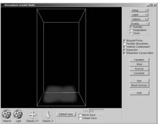
3.3
Interface
Our graphical user interface for the cloud modeling soft-ware application has been implemented using the GLUI in-terface toolkit[16] on top of OpenGL. The user has the abil-ity to change view parameters, as well as bring up additional
Figure 4. 2D example of momentum conser-vation algorithm.
menus for simulation parameters that can be modified dur-ing the simulation. This allows the user maximum control over the simulation environment during run-time. An ex-ample of our GUI is shown in figure 5.
Figure 5. Graphical User Interface
We have also included an interface for manipulating wind in the environment—both a global directional wind and a local cross-wind which can be set to high speed and aperture to create a desired amount of turbulence. We have also included an additional scalable random motion to our velocity field. The user is also able to customize the heat source configuration at ground level and set the source of humidity–either entering from just above sea level (evapo-ration) or incoming from cross-winds. In our implementa-tion we use a Perlin noise funcimplementa-tion scaled by an overall con-centration value to define both of our humidity sources[15]. Perlin noise is a more natural source for an initial random distribution than a uniform block of density.
In our application, volumetric data is rendered interac-tively using smooth-blended transparent billboards gener-ated from back to front. However, the volumetric data
gen-erated can be exported for off-line rendering using any vol-ume rendering algorithm8.
4
Creating Different Cloud Types
Cloud formation is a scene with many “actors” in it. Consequently, there are many distinct ways that the actors in the atmosphere can interact to form clouds. This is why dif-ferent atmospheric conditions produce difdif-ferent cloud for-mations. Currently our simulation focuses only on two main cloud types—cumulus clouds and stratus clouds. Cumulus clouds are formed by vertical air movement caused by ther-mal currents over land. Stratus clouds, on the other hand, are formed by horizontal wind currents over oceans or other large bodies of cold water. We will explain in detail how we set up our environment to form each cloud type.
4.1
Creating Cumulus Clouds
We form cumulus clouds by defining a plume of humid-ity and a heat source at ground level. The incoming heat raises the temperature of the air and buoyancy causes the humid air to rise. The heat source pattern can be tailored to fit the approximate cloud shape desired. As the humid-ity rises and begins to condense, latent heat is released, increasing the upward buoyant force and producing a pre-dominantly vertical cloud growth pattern. In our simulation we have included wind to help shape the cloud as well. A global wind defines the drift pattern of the cloud, while local crosswinds introduce turbulence into the environment. We have also implemented a vorticity confinement algorithm presented by Steinhoff and Underhill[19] which helps pre-serve the appearance of swirling effects caused by conserv-ing momentum under turbulent conditions. Figure 6 shows an example of cumulus cloud formation.
Figure 6. Cumulus cloud formation caused by vertical air movement.
8Data resampling may be advantageous to give better volume-rendering results
4.2
Creating Stratus Clouds
Stratus clouds are formed slightly differently than cumu-lus clouds. Stratus clouds usually form over cold terrain such as ocean water, where there is little or no vertical air movement. Contrary to the cumulus cloud set-up, for stra-tus clouds we do not define any heat source for our environ-ment and our source of humidity is outside our simulation region, carried in on a horizontal cross-wind. The user can define the direction and altitude of the cross-wind and also the amount of humidity carried in by the wind. This gives us humidity traveling horizontally instead of vertically. When any of the water vapor condenses, the latent heat released causes some buoyancy and therefore we see wispy streaks of cloud, interspersed horizontally around the dew point. Figure 7 is an example of stratus cloud formation.
Figure 7. Stratus cloud formation caused by horizontal air flow.
4.3
Performance Analysis
The above images were rendered interactively on a grid size of 15x50x15 and 50x15x15, respectively, at an approx-imate frame rate of 1 frame/sec on a standard desktop PC9.
This is usually an acceptable frame for interactive modeling of the cloud. Frame rates can be increased by using lower grid sizes or more powerful hardware.
5
Rendering
The volumetric data produced by our method is far from a finished product in terms of artificial clouds. Our im-plementation provides only a fast OpenGL-based rendering method that is useful for quickly examining the cloud for design purposes. In order to be more useful, this data must be exported for use in advanced rendering applications. The data that we have produced—a three-dimensional grid of 9Pentium III 800MHz processor with 256Mb RAM and a Geforce 2 graphics accelerator
density data—serves as a low-level representation of the fin-ished product. Rendering techniques should be used wisely to create not only lighting and shading effects, but also to create added detail for finished clouds. In section 5.1 and section 5.2 we present an example of exporting our data to an external rendering engine. In this case we have used the SkyWorks source provided by Mark Harris of the Univer-sity of North Carolina.
5.1
Data Processing Steps for Rendering
We have implemented several ad hoc methods to pre-pare our data for the given rendering application. Besides resampling our data, we must also convert our grid format to a particle structure, as this is the input required for ren-dering using SkyWorks. Additionally, we may also want to apply other filters to redistribute the density values of a given cloud.
First, we have used a standard trilinear interpolation method with a gaussian filter to resample and smooth our initial volumetric data. This allows us to enhance the reso-lution of the rendered model. On average, we have no more than doubled the initial resolution for each axis.
Next we must convert our data to the required particle format. For this we have implemented a simple pattern search that operates on our volume data. After initially cre-ating a particle for each grid point, the algorithm searches for groups of eight juxtaposed particles (that have not yet been processed). When this pattern is found, a new, larger particle is created with a density value equivalent to the av-erage of the previous eight particles. When rendering with imposters, the number of particles used will always affect the overall opacity of the object, therefore we would like to build a cloud with only as many particles as are required to define the shape. On average, the simple method we have implemented decreased approximately 5K grid-sized parti-cles to approximately 1.5K variable size partiparti-cles.
Finally, we have also implemented a density resampling routine. This affects the perceived boundary of the cloud by redefining the fall-off rate for density opacity values. For example, we can create an exponential fall-off by simply squaring our density values. Alternatively, we can create another smooth fall-off by computing the tan() of our densi-ties. Since our density values are defined on the scale [0,1], any function whose range is [0,1] on the given domain can be used. Our given results have used an exponential filter.
5.2
Rendering using SkyWorks
As we have previously mentioned, the SkyWorks ren-dering engine renders static clouds10, therefore in order to
10The reason for this is that the method implemented by Mark Harris requires illumination tables to be precomputed for each cloud.
assemble a video sequence of cloud formation using this engine we were required to create a batch process to ex-port images of each volume frame (exex-ported from our ap-plication), and then assemble those frames as a sequence. Because our particle conversion method is not continuous from frame to frame, a heavy motion blur was also applied. As expected, the SkyWorks rendering engine achieved excellent interactive frame rates for static cloud images, av-eraging over 100 frames per second when navigating 3-5K element clouds. In the static view, however, our clouds were not quite as pleasing in appearance as the hand-painted clouds used in the SkyWorks demo11. However, our
assem-bled video sequences of cloud formation show that our ap-plication can be used to create realistic simulations of cloud formation.
6
Future Work
In this section we discuss several directions for further research.
q
More cloud types
There are many more types of cloud formations than just the two we have addressed in our current simula-tion. These include cirrus, cirrocumulus, cirrostratus, altocumulus, altostratus, nimbostratus, stratocumulus, and cumulonimbus[21]. As the names suggest, many of these cloud types are variations of the three main cloud formations: stratus, cumulus, and cirrus. Al-though we have not yet explored creation of these other types, we believe our model should easily adapt to han-dle them. With additional research we would like to add environmental presets for each cloud type to aid the user in creating these different base types. In addi-tion, our fluid simulator should support simulation of wind patterns over rough terrain, which should enable us to create clouds formed by orographic uplift.
q
Complete growth cycle including precipitation and dissipation
We also hope to add to the current growth cycle of our clouds. Once enough water vapor has condensed into cloud form, gravity starts to pull down on some of the larger condensed particles. As the large droplets fall through the cloud colliding with other condensed particles, the process of precipitation begins[21]. We would like to experiment with modeling the precipita-tion stage of the cloud life cycle in our model, perhaps with an overlaid particle system. This would not only include rain but also other forms of precipitation in-cluding snow and frozen rain.
11SkWorks demo available at
http://www.cs.unc.edu/ harrism/clouds/RTCRDownload.html
q
More research into atmospheric model
By improving our model of the atmosphere, we will be able to better mimic the complex processes that con-tribute to the formation of other cloud types and storm systems. We would like to improve our model to the point that we are able to successfully incorporate all three stages of the thunderstorm lifecycle described by Byers and Braham[1]: the cumulus stage, the mature stage, and the downdraft stage. We are also exploring possible ways of simulating density differences in the atmosphere and their effects on our system.
q
Gesture interface for artistic creation of environment We would like to conduct some user experiments with a three-dimensional augmented reality interface in which the user is able to interact with the environ-ment by means of a gesture-based interface. Using such an interface the user would be able to more accu-rately shape the volumetric structure (e.g. by “seeding” hygroscopic nuclei) of the cloud during the course of the simulation.
q
Incorporation of large-scale weather simulation Our current simulator is geared toward the creation of individual or small groups of clouds over a lim-ited region. By simulating the weather patterns over a larger region, it is possible to define “regions of in-terest” where different cloud types will form. We plan to perform such a large-scale simulation to provide au-tomated input data for our small-scale simulator. In this way, we should be able to populate a sky with a set of realistic, physically-based clouds.
7
Conclusions
We have developed an efficient physically-based simu-lation of cloud formation which can be run interactively on a standard desktop PC. This model provides a basis for interactively modeling physically-based clouds in 3D us-ing a computational fluid solver. While we have presented our model in conjection with a specific Navier-Stokes fluid solver, this model can in fact be used with any grid-based fluid solver. Our model is one of few to date which has ad-dressed more than one type of cloud. We believe that the proposed model is a significant improvement over previous models of cloud formation in the field of Computer Graph-ics and hope to improve this model in the future.
Acknowledgements
We would like to thank everyone who has contributed to this project, including Dr. Mike Biggerstaff of the Texas
A&M Meteorology Department, Mark Harris of the Univer-sity of North Carolina for his ongoing help with rendering, and Dr. Darryl Overby for his help with fluid dynamics.
Appendix A
In this section we give a brief overview of the Navier-Stokes equations for those who may be unfamiliar with them.
When building a model of fluid flow, we will begin by assuming that mass is fully conserved. This means that the net change in mass must always be zero. This is expressed mathematically in equation 7. This equation states that the time rate of change in density (rs
r)t
) is balanced by the diver-gence of the mass flux at any point in space.
uwvHx vHy z|{~} xU 22 (7) x
is the density and
is the vector representing velocity within the fluid. If we assume that our density is constant (i.e. rs
r)t z
), non-zero, and varies gradually compared to changes in velocity, then equation 7 simplifies to:
{~}
z
(8) This equation expresses conservation of mass within our system, and is required for the system to be properly con-strained. There are four unknowns in the fluid system, pres-sure and velocity in the x,y,z directions, and thus we need four equations. Equation 8 coupled with the three Navier-Stokes equations constitute a complete solution for fluid flow. The Navier-Stokes equations can be written together as shown below in equation 9[22].
vH vHy }{ z u {Y x { x (9) The terms on the left of the equation are our inertial celeration terms. The first term expresses our temporal ac-celeration while the second expresses spatial effects within the system. On the right is a pressure term followed by a term which expresses the viscous force (shear stress). The final term represents any external forces per unit volume applied to the system. This equation shows that motion within the system is dependant upon force due to pressure, force due to viscous effects, and force due to any external forces such as gravity (or buoyancy). Because the inertial effects outweigh the contribution of viscous effects in air, we can ignore the viscous term. To see this we examine the Reynolds number for our system. The Reynolds number ex-presses the dimensionless ratio of inertial forces to viscous forces and is given as [22]:
C
z
})
(10)
where u is a characteristic velocity and L is characteris-tic length and
is kinematic viscosity12. For air at approx-imately
U)
,
z-g+
[22]. Also, since the troposphere extends approximately
-
from the surface of the earth[21], we will use
as our (very conserva-tive estimate of) characteristic length. Therefore, in order for the Reynolds number to be 1.0 (where the inertial effect equals that of the viscous effect), our flow speed would have to remain below +
. Since the fluid motion we will be modeling will be much faster than this, we can assume that C2
and therefore viscous effects can be ignored. Looking at the Navier-Stokes equation again, we can see that, having removed the viscous term, our inertial accelera-tion in the system will be balanced by pressure and external forces within the system. This makes our fluid flow com-putation much easier since we do not have to compute the effects of viscosity.
Appendix B
The basic steps of our simulation:
Initialize grid space. Initialize each voxel’s:
– Velocity – Humidity – Heat – Condensation Simulation Loop:
– Source Step. Add external velocity forces based
on:¡ Wind ¡ Vorticity Confinement ¡ Buoyancy
– Simulation Step. Handles motion of fluid based
on Stam’s model [17]¡
Transport Step – Handle Periodic Bound-aries
¡
Diffusion/Dissipation Step
¡
Momentum Conservation Step
¡
Expansion Step
¡
Projection Step
– Compute relative humidity
12Kinematic viscosity is defined as the fluidic viscosity of the material divided by the density[22]
– Condense water ¢ Compute condensation ¢ Reduce humidity ¢
Add latent heat
References
[1] H. Byers and R. B. Jr. Thunderstorm structure and circula-tion. J. Meteor, 5:71–86, 1948.
[2] Y. Dobashi, K. Kaneda, H. Yamashita, T. Okita, and T. Nishita. A simple, efficient method for realistic animation of clouds. Proc. of SIGGRAPH 2000, pages 19–28, 2000. [3] D. S. Ebert, F. K. Musgrave, D. Peachey, K. Perlin, and
S. Worley. Texturing & Modeling. AP Professional, 2nd edition, 1998.
[4] R. Fedkiw, J. Stam, and H. W. Jensen. Visual simulation of smoke. Proc. of SIGGRAPH 2001, pages 15–22, 2001. [5] G. Gardner. Visual simulation of clouds. Proc. of
SIG-GRAPH ’85, pages 297–303, 1985.
[6] M. Harris and A. Lastra. Real-time cloud rendering. Com-puter Graphics Forum (Eurographics ’01 Proc.), 20(3):C– 76–C–84, 2001.
[7] W. B. B. Jr. A Primer in Fluid Mechanics: Dynamics of Flows in One Space Dimension. CRC Press, 1999. [8] J. Kajiya and B. V. Herzen. Ray tracing volume densities.
Proc. of SIGGRAPH ’84, pages 165–174, 1984.
[9] K. Kaneko. Simulating physics with coupled map lattices— pattern dynamics, information flow, and thermodynamics of spatiotemporal chaos.
[10] J. Lewis. Algorithms for solid noise synthesis. Proc. of SIGGRAPH ’89, pages 263–270, 1989.
[11] R. Miyazaki, S. Yoshida, Y. Dobashi, and T. Nishita. A method for modeling clouds based on atmospheric fluid dy-namics. Pacific Graphics, 2001.
[12] K. Nagel and E. Raschke. Self-organizing criticality in cloud formation? Physica A, 182:519–531, 1992.
[13] F. Neyret. Qualitative simulation of convective cloud forma-tion and evoluforma-tion. Eurographics, 1997.
[14] T. Nishita, Y. Dobashi, and E. Nakemae. Display of clouds taking into account multiple anisotropic scattering and sky light. Proc. of SIGGRAPH ’96, pages 379–386, 1996. [15] K. Perlin. Hypertexture. Proc. of SIGGRAPH ’89, pages
253–261, 1989.
[16] P. Rademacher. Glui interface toolkit.
[17] J. Stam. Stable fluids. Proc. of SIGGRAPH 99, pages 121– 128, 1999.
[18] J. Stam and E. Fiume. Depiction of fire and other gaseous phenomena using diffusion processes. Proc. of SIGGRAPH ’95, pages 129–136, 1995.
[19] J. Steinhoff and D. Underhill. Modification of the euler equations for “vorticity confinement”: Application to the computation of interacting vortex rings. Physics of Fluids, 6(8):2738–2744, 1994.
[20] J. Wallace and P. Hobbs. Atmospheric Science: An Intro-ductory Survey. Academic Press, 1977.
[21] R. N. Wallen. Introduction to Physical Geography. Wm. C. Brown Publishers, 1992.
Figure 8. Humidity field being advected by buoyancy.
Figure 9. Heat Field. Notice added heat where condensation occurs.
Figure 10. Resulting Cloud Field.