with non-linear partial differential
equations
vorgelegt von Diplom-Mathematiker
Kevin Sturm
aus Rathenow an der Havel
Von der Fakult¨at II – Mathematik und Naturwissenschaften der Technischen Universit¨at Berlin
zur Erlangung des akademischen Grades
Doktor der Naturwissenschaften – Dr.rer.nat. –
genehmigte Dissertation
Promotionsausschuss:
Vorsitzender: Prof. Dr. Wolfgang K¨onig Gutachter: Prof. Dr. Dietmar H¨omberg Gutachter: Prof. Dr. Michael Hinterm¨uller Gutachter: Prof. Dr. Michel C. Delfour
Tag der wissenschaftlichen Aussprache: 9. Oktober 2014
Berlin 2015 D83
This thesis is concerned with shape optimization problems under non-linear PDE (partial differential equation) constraints.
We give a brief introduction to shape optimization and recall important concepts such as shape continuity, shape derivative and the shape differentiability. In order to review existing methods for proving the shape differentiability of PDE constrained shape functions a simple semi-linear model problem is used as constraint. With this example we illustrate the conceptual limits of each method.
In the main part of this thesis a new theorem on the differentiability of a minimax function is proved. This fundamental result simplifies the derivation of necessary optimality conditions for PDE constrained optimization problems. It represents a generalization of the celebrated Theorem of Correa-Seeger for the special class of Lagrangian functions and removes the saddle point assumption. Although our method can also be used to compute sensitivities in optimal control, we mainly focus on shape optimization problems. In this respect, we apply the result to four model problems: (i) a semi-linear problem, (ii) an electrical impedance tomography problem, (iii) a model for distortion compensation in elasticity, and finally (iv) a quasi-linear problem describing electro-magnetic fields.
Next, we concentrate on methods to minimise shape functions. For this we recall several procedures to put a manifold structure on the space of shapes. Usually, the boundary ex-pression of the shape derivative is used for numerical algorithms. From the numerical point of view this expression has several disadvantages, which will be explained in more detail. In contrast, the volume expression constitutes a numerically more accurate representation of the shape derivative. Additionally, this expression allows us to look at gradient algorithms from two perspectives: the Eulerian and Lagrangian points of view. In the Eulerian ap-proach all computations are performed on the current moving domain. On the other hand the Lagrangian approach allows to perform all calculations on a fixed domain. The La-grangian view naturally leads to a gradient flow interpretation. The gradient flow depends on the chosen metrics of the underlying function space. We show how different metrics may lead to different optimal designs and different regularity of the resulting domains.
In the last part, we give numerical examples using the gradient flow interpretation of the Lagrangian approach. In order to solve the severely ill-posed electrical impedance tomography problem (ii), the discretised gradient flow will be combined with a level-set method. Finally, the problem from example (iv) is solved using B-Splines instead of level-sets.
This dissertation thesis is a result of 3 years research in the groupNonlinear Optimization and Inverse Problemsat theWeierstrass Institute for Applied Analysis and Stochastics Leib-niz Institute in Forschungsverbund Berlin e.V., located in Berlin, Germany. The presented results were obtained within the work of Matheon research project C11 – Modeling and optimization of phase transitions in steel supported by the DFG research center Matheon Mathematics for key technologies.
I would like to express the deepest appreciation to supervisor Professor Dietmar H¨omberg who supported me to explore my own ideas. He encouraged me to attend conferences and introduced me to many interesting people. In this regard, he introduced me to Professor Jan Soko lowski who triggered the creation of Chapter4, the core of this thesis, and helped me with mathematical issues. Some months later, in a conference meeting in Erlangen, I had the opportunity to meet Professor Michel Delfour who helped me to extend the results from Chapter 4. Further I would like to acknowledge Professor Michael Hinterm¨uller for his help with the example of Chapter5.2. Also I would like to thank Dr. Antoine Laurain and Dr. Martin Eigel with whom I had many discussions that resulted in the Chapters 6 and 7of this thesis. Of course I also would like to thank my co-workers at the WIAS and at the Technical University Berlin. A special thanks to Anke Giese for her patience. A great thanks to Wenxiu for her patience and support. Finally, I wouldn’t be here without my beloved parents who gave me continuous support.
1 Introduction 2
2 Introduction to shape optimization 8
2.1 Notation . . . 8
2.2 General shape optimization problems . . . 11
2.3 Flows, homeomorphism and a version of Nagumo’s theorem . . . 12
2.4 Shape continuity . . . 19
2.5 Sensitivity analysis . . . 25
3 Shape differentiability under PDE constraints 31 3.1 The semi-linear model problem . . . 31
3.2 Material derivative method . . . 32
3.3 Shape derivative method. . . 36
3.4 The min-max formulation of Correa and Seeger . . . 38
3.5 C´ea’s classical Lagrange method and a modification . . . 42
3.6 Rearrangement of the cost function . . . 43
3.7 Differentiability of energy functionals . . . 44
4 Shape derivative via Lagrange method 46 4.1 An extension of the Theorem of Correa-Seeger . . . 46
4.2 More theorems on the differentiability of Lagrangians . . . 53
4.3 Continuity and Lipschitz continuity oft7→xt . . . 56
5 Applications to transmission problems 62 5.1 The semi-linear model problem . . . 62
5.2 A transmission problem in elasticity . . . 65
5.3 Electrical impedance tomography . . . 76
5.4 A quasi-linear transmission problem . . . 83
6 Minimization using the volume expression 95 6.1 A glimpse at the Michelletti construction . . . 95
6.2 Groups of diffeomorphisms via velocity fields . . . 97
6.3 Gradient flow andH-gradient . . . 103
6.4 Descent directions and the H-gradient . . . 105
6.5 Lagrangian vs. Eulerian point of view . . . 108
6.6 Translations and rotations . . . 115
6.7 Splines and theH-gradient . . . 116
6.8 The level set method . . . 119 vii
Contents 1
7 Numerical simulations 121
7.1 Unconstrained volume integrals: gradient methods . . . 121
7.2 A transmission problem: gradient method and volume expression . . . 122
7.3 The EIT problem: level set method and volume expression . . . 123
7.4 Distortion compensation via optimal shape design using basis splines . . . . 125
8 Appendix 133 A Measure spaces . . . 133
B Bochner integral . . . 134
C Sobolev spaces . . . 135
Introduction
He who seeks for methods
without having a definite problem in mind seeks in the most part in vain.
David Hilbert
Shape optimization
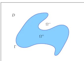
Shape optimization has gained an increasing attention from the theoretical and application points of view. Many problems from real world applications can be recasted as shape optimization problems. It has proved its indispensability in many applications such as drag reduction of aircrafts, cars and boats, electrical impedance tomography [32,54] and image segmentation [56].
In general, a shape optimization problem consists of a cost/shape function J(Ω, u(Ω)) with arguments Ω⊂Rdandu(Ω), where thestate usatisfies theconstraint E(Ω, u(Ω)) = 0. The objective then is to minimize the cost functionJ : Ξ→Rover someadmissible subset
Ξ of 2Rd :={Ω : Ω⊂Rd}, i.e.
minimizeJ(Ω, u(Ω)) over (Ω, u)∈Ξ× X(Ω)
subject to u=u(Ω) solvesE(Ω, u(Ω)) = 0, (1.1) whereX(Ω) is usually a function space. The constraintE(Ω, u(Ω)) = 0 could be a partial differential equation (PDE) or systems of PDEs such as the Navier-Stokes equation [84] or Maxwell’s equations [53,102]. A specific Ξ could be the set of all open subsets of a setD. A unique characteristic of shape optimization is that it makes bonds from different areas of mathematics, such as differential geometry, Riemmanian geometry, real and complex analysis, partial differential equations, topology and set theory. The main difficulty arises because of the absence of a vector space structure of the set of sets 2Rd. Thus one cannot apply standard tools from real analysis such as the Fr´echet or the Gateaux derivative to investigate (1.1). One may circumvent this obstacle by identifying sets with functions and giving the space of these functions aLie group ormanifold structure as detailed below; cf. [37,72,73,95].
In order to study the behavior of shape functions with respect to domain variations
shape sensitivity analysis was introduced. In [100] the hereafter described velocity method was adopted for this purpose. We refer to [90] for the computation of material derivatives for various PDEs. Let a shape function J : Ξ→R on some admissible set Ξ⊂ {Ω : Ω⊂
D ⊂ Rd} and a set Ω ⊂D contained in a bigger set D be given. Then the domain Ω is 2
3
perturbed by a suitable family of diffeomorphisms Φt :D →D, t≥0, with Φ0 = id. The result is a family of new domains Ωt:= Φt(Ω), t≥0. One may define the diffeomorphisms
Φt as the flow of a vector field θ:D → Rd. We define then the Eulerian semi-derivative
(if it exists) as limit
dJ(Ω)[θ] := lim
t&0
J(Ωt)−J(Ω)
t .
If the mapθ7→dJ(Ω)[θ] is linear and continuous, then it is termedshape derivative. Shape sensitivity was first used by Hadamard in his study of elastic plates; cf. [49]. The famous “structure theorem” of shape optimization states that under certain assumptions the shape derivative is a distribution acting on the normal part θ·n of the perturbation field θ on the boundary ∂Ω. In 1907, J. Hadamard [49] used displacements along the normal to the boundary Γ of a C∞-domain to compute the derivative of the first eigenvalue of the clamped plate. The structure theorem for shape functionals on open domains with aCk+1 -boundary is due to J.-P. Zol´esio [101] in 1979. The generalization of the structure theorem to an arbitrary domain was done in the paper [40, Thm. 3.2 and Rem. 3.1, Cor. 1] in 1992. It says that the shape gradient is a finite order distribution with support the boundary of the set and normal to the boundary.
In most cases, when the boundary is regular enough the boundary expression may be written in integral form
dJ(Ω)[θ] = Z
∂Ω ˜
g n·θ ds, (1.2) where ˜g : Γ →R is usually the restriction of a function defined in a neighborhood of ∂Ω. The formula (1.2) is often called the Hadamard formula.
Forstate constrained shape optimization problems, where the state is a partial differen-tial equation, the shape differentiability may be difficult to prove depending on the PDE. One procedure is to derive the shape differentiability as follows. One may express the cost functiong(z) (zbeing an element of a topological vector space) of PDE constrained shape optimization problems as a minimax of a Lagrangian functionG taken over vector spaces X and Y, i.e.,
g(z) = min
x∈Xmaxy∈Y G(z, x, y).
The problem of the shape differentiability of the cost function is transported to the differ-entiability of the minimax. Theorems on the differdiffer-entiability of a minimax function with or without saddle point condition have a long history. The pioneering work in this area was done by Demjanov (cf. [42]) as early as 1968. Correa and Seeger gave in [30] a di-rect theorem on the differentiability of g(z), where z ∈ Z, Z a locally convex space, and (x, y) ∈ X×Y , X and Y two Hausdorff topological spaces (see also methods of non-smooth analysis in their bibliography). Since spaces of shapes or domains are not locally convex spaces1, [36] reformulated the hypotheses of the previous theorems to make them readily applicable to the computation of the shape derivative. Some of those theorems were sharpened by Delfour and Morgan [33, Thm. 3] and extended to -solutions in [34]. In [35] an interesting penalization method was introduced where the state is the solution of a variational inequality. We would like to emphasize that until now none of the mentioned methods are applicable to non-linear problems without further assumptions, such as that Ghas saddle points.
Other methods which may be used to derive the shape differentiability are the following:
1
In fact certain spaces of shapes can be identified as infinite dimensional Riemannian manifolds. We come back to this topic in Chapter6.
1. The “chain rule approach” or material derivative method is as follows. In this ap-proach thematerial derivative is introduced to derive the shape differentiability. The material derivative can be interpreted as the derivative of the state with respect to the domain and only occurs in an intermediate step and is not present in the final formula of the shape derivative. The terminology of the material derivative originates from continuum mechanics where it describes the time rate of change of some physical quantity, such as the mass, for a material element subjected to a time dependent ve-locity field. From the optimal control point of view this is nothing but the derivative of the control–solution operator, where the control is the domain and the solution is some function solving a PDE.
2. Another (formal) method that is often used to derive the boundary expression, which has to be used with caution because itmay yield the wrong formula2 is due to [23]. This method, also known as C´ea’s Lagrange method, uses the same Lagrangian as the minimax formulation, but requires that the shape derivatives of the state and the adjoint equation exist and belong to the solution space of the PDE. There are examples (see [82]), where C´ea’s Lagrange method fails.
3. In the recent paper [60] a rearrangement method was proposed. This method allows to prove the shape differentiability under the assumption that the domain-solution operator is H¨older continuous with an exponent bigger than 1/2 and admits a second order expansion with respect to the unknown. No convexity of the state or the cost is needed. However it requires a first order expansion of the PDE and cost function with respect to the unknown such that the remainder vanishes with order two. Finally, we mention that there is an interestingpenalization method introduced in [35].
Current trends
A natural way to deal with domains is by identifying them with functions. There are several methods to identify domains with functions, two of these will be further explained for the planar case ofR2.
In the first approach simply connected domains Ω in the plane, with boundary Γ, are identified with immersed or embedded3 curves γ which map from the circle S1 onto the boundary Γ as done in [72]. Since a reparametrization of the curve does not af-fect the image Γ one is led to consider equivalence classes of curves. Two curves are equivalent, written γ ∼ γ˜, if there exists ϕ ∈ Diff(S1) such that γ = ˜γ ◦ϕ. The space Be := Emb(S1;R2)/Diff(S1) comprising equivalence classes of embedded curves is a special
case of a manifold of mappings. It can be given a Riemannian structure by introducing appropriate metrics; [71, 73, 93, 98]. With the identification of domains Ω ⊂ R2 with functions γ ∈ Be, we may identify a shape function J(Ω) with ˜J(γ) := J(int(c)), where
int(γ) is the interior of Γ := ∂Ω, that is, Ω. The link between the shape derivative in the form (1.2) and the derivative of ˆJ on the shape space Be was given by [86]. The main
benefit of this view is that on Riemannian manifolds minimization methods such asBFGS4, steepest descent, Newton and quasi-Newton methods as well as their convergence analysis are available; cf. [2,85,86].
2We come back to this method in Subsection3.5. 3
The quotientBi:= Imm(S1;R2)/Diff(S1) is no manifold, but only an orbifold.
4
5
An alternative approach of [70] defines admissible domains Ω⊂R2by Ω = (f+ id)(ω 0), f ∈ C0k(R2,R2), k ≥ 1 and some fixed open domain ω0 ⊂ Rd. Formally, setting Θ := Cb0,1(Rd,Rd)5, an appropriate space is given by
F(Θ) :={id +f : f ∈Θ, f+ id is bijective and (f+ id)−1−id∈Θ}.
Since one is usually interested in the image of the mappings, we consider the groupSω0 :=
{F ∈ F(Θ) : F(ω0) = ω0}. Now we introduce the equivalence relation between two functionsF,F˜∈ F(Θ), writtenF ∼F˜ byF◦h= ˜F for some h∈ Sω0. As for the spaceBe
the important role plays the quotient He := F(Θ)/Sω0 on which a right invariant metric,
called Courant metric, can be introduced to make the space He a complete metric group
[37]. The equivalence relation is nothing but the right action ofSω0 on the groupF(Θ) and
induces a natural projection π :F(Θ)→ F(Θ)/Sω0, byf 7→f ◦ Sω0. By construction, we may identify the quotientF(Θ)/Sω0 with the image setZ(ω0) :={F(ω0) : F ∈ F(Θ)} via
the bijectionF 7→F(ω0).
In 1993, the problem of comparing medical scans arising in medical imaging led to the construction of deformations defined byϕ(x) :=x−u(x), whereuis a smooth displacement in the plane [69] which is smoothed by a Sobolev type energy minimization. Since this displacement allows not for arbitrary large deformations the velocity method was used by [14,95] to construct deformations via the flow of a vector fields. More precisely the authors considered the group G := {Φθ1 : θ vector field} of all flows evaluated at t = 1. Also in this case a right invariant metric may be introduced making the spaceG a complete metric group.
Finally, we mention that spaces of shapes can also be generated by distance functions, signed distance functions and characteristic functions, but lead to less differentiable struc-tures.
The previous considerations show that by identifying sets with functions, we can employ most of the features from smooth analysis on infinite dimensional manifolds. This will be a cornerstone for future numerical and theoretical investigations of constrained shape optimization problems.
The objective of this thesis
The main contributions of this thesis are:• In this thesis, we present a novel approach to the differentiability of a minimax, with-out a saddle point assumption when the functionGis a Lagrangian, that is, a utility function plus a linear penalization of the state equation. Until now the assumptions to apply the minimax theorems required that the Lagrangian is a concave-convex func-tion or other hypotheses have to be satisfied that are not easy to be proved or even fail to be true. The novelty of the new approach is to replace the usual adjoint state equation by an averaged adjoint state equation. For problems where the function is a Lagrangian this result allows us now to compute sensitivities for a very broad class of shape optimization problems contained by linear, semi-linear and also quasi-linear partial differential equations.
• Most numerical simulations use the boundary expression (1.2) or to be more precise the pointwise descent directionθ:=−g n. It is well known that due to low regularity of
5
The spaceCc0,1(Rd,Rd) comprises all bounded Lipschitz continuous functionsf:Rd→Rd. This space is a Banach space when endowed with the usual norm.
gthe algorithm may be unstable and can lead to oscillations of the moving boundary. The low regularity of g may occur if Ω is less regular or the cost function involves high order derivatives of the solution of the PDE or the solution of the PDE has low regularity. Besides introducing penalizations, one way to get around this is to consider the alternative representation of the shape derivative as a domain integral, i.e. dJ(Ω)[θ] =R
ΩF(θ)dx, where F is an operator acting on θ. This expression is more general than the boundary expression and is even defined for quite irregular domains Ω, where no boundary expression is available. It has been overlooked for mainly two reasons:
- the difficulty to obtain descent directions,
- the computational effort seems to be bigger since a space dimension is added. We will make the volume expression accessible for numerical simulations. Also we discuss why the volume expression is advantageous when combined with the level-set method.
• With the volume expression it is possible to interpret gradient algorithms as gradient flows taking values in certain groups of diffeomorphisms. This interpretation allows us to distinguish between two different ways to look at gradient algorithms: (i) from the Eulerian and (ii) from the Lagrangian. In the Eulerian approach all computations in an algorithm are performed on the current domain. On the other hand the Lagrangian approach allows to perform all calculations on a fixed domain. The gradient flow depends on the chosen metric of the underlying space. We present several possible metrics and different regularity of the resulting domains.
The structure of this thesis
Outline:Chapter 2: This chapter gives a brief introduction to shape optimization is given and recalls some basic material from shape calculus. The essential notation used throughout this thesis is introduced. We introduce the notion of the shape derivative and the structure theorem of Zol´esio. Many useful properties of the flow associated with vector field are derived. Chapter 3: In this chapter various methods available to calculate the so-called shape deriva-tive are reviewed. The methods range from the classical material derivaderiva-tive method [90] (also called chain rule approach), over the minimax approach of Correa-Seeger applied to shape optimization by Delfour and Zol´esio ([36]), to the recent rearrangement method of [60]. Finally, we consider a theorem on the differentiability of a min function, that allows the calculation of sensitivities for energy functionals. In order to illustrate the methods a simple quasi-linear partial differential equation is used.
Chapter 4: A novel approach to the differentiability of a minimax, without a saddle point assumption when the function is a Lagrangian, that is, a utility function plus a linear pe-nalization of the state equation, is presented. Its originality is to replace the usual adjoint state equation by an averaged adjoint state equation. When compared to the former the-orems in [36, Sect. 4, Thm. 3, p. 842] and in [33, Thm. 3, p. 93], all the hypotheses are now verified for a Lagrangian function without going to the dual problem and it relaxes the classical continuity assumptions on the derivative of the Lagrangian involving both the state and adjoint state to continuity assumptions that only involve the averaged adjoint state.
7
Chapter 5: The results from Chapter 4 are applied to three transmission problems and the semi-linear problem from Chapter 3: (i) a sharp interface model of distortion com-pensation in elasticity (ii) an electrical impedance tomography problem, (iii) a quasi-linear transmission problem and (iv) a simple quasi-linear problem. For the examples (i) – (iii) the existence of optimal shapes via a standard perimeter and a Gagliardo penalization (also called fractional perimeter penalization) is discussed.
Chapter 6: This chapter deals with the theoretical treatment of shape optimization prob-lems. The novel part is the usage of the volume expression of the shape derivative, which has been ignored so far. We compare different metrics generating gradient flows in the spaces of shapes.
Chapter 7: The methods introduced in Chapter 3 are applied to the examples introdcued before. It is shown that the volume expression is superior when compared to the boundary expression.
Introduction to shape optimization
In this chapter, we introduce shape functions along with an appropriate notion of continuity and differentiability. We recall the celebrated structure theorem of Hadamard-Zol´esio which provides us with the canonical structure of shape derivatives. Finally, we study flows generated by vector fields. For the convenience of the reader, we list below all used symbols and function spaces.2.1
Notation
We mostly use notations and definitions of the Amman-Escher book series [7,8,9]. Some definitions can be found in [37]. Let f : Ω ⊂ Rd → Rd and φ : Ω ⊂ Rd → R be given
functions defined on a set Ω with boundary Γ.
• Measures and sets:
N,Z,R natural numbers, integers, real numbers
R,R+ extended (non-negative) real numbersR∪ {±∞}
and{x≥0} ∩R∪ {∞}
Rd d- times product ofR
E, F Banach spaces with normsk · kE,k · kF
int(Ω), ∂Ω, Ω interior, boundary and closure of a set Ω⊂Rd 2Ω set of all subsets of Ω, i.e.,{Ω : ˜˜ Ω⊂Ω}
TD(x), CD(x) Bouligand and Clarke tangent cone ofDatx∈D
supp(φ) support of a function φ, i.e., {x∈Rd: φ6= 0}
YX set of all functions fromX intoY
bsc the biggest integer less or equal to s df(x;v) directional derivative off : Ω⊂E →F
atx∈Ω in direction v
dHf(x;v) Hadamard semi-derivative atx∈Ω in directionv ∈E ∂f(x) Fr´echet derivative at x; it is an element of L(E, F) ∂γf(x) partial derivative ∂ |γ|f ∂γ1x 1···∂γdxd, where γ = (γ1, . . . , γd) >∈Nd and|γ|:=γ1+· · ·+γd
∇φ gradient defined by∂f(x)(v) =∇φ·v for allv∈Rd
∇Γφ tangential gradient∇φ|Γ−∂nφ|Γn 8
2.1. Notation 9 ∂Γf|Γ tangential gradient∂f|Γ−(∂nf)⊗n ε(f) symmetrised gradient 12(∂f +∂f>) J rotation matrix 0 1 −1 0 !
A>, A−1 transpose and inverse of a matrix
•Function spaces:
L(E,F) space of linear and continuous mappings fromE intoF
Lis(E,F) space of mappingsA∈ L(E,F) with inverse A−1∈ L(F,E)
Ck(Ω) space of k-times continuously differentiable mappings from Ω intoR Cck(Ω) space of functionf ∈Ck(Ω) such that suppf ⊂Ω
C0,α(Ω) H¨older space with exponent 0< α <1 (also denoted Cα(Ω))
Ck,α(Ω) subspace of functionf ∈Ck(Ω) such that the k-th order derivatives
belong toCα(Ω), 0< α <1,k≥0
C(Ω) space of continuous functions that are bounded on Ω Lp(Ω) standard space of measurable function that are p-integrable
(1≤p <∞)
L∞(Ω) space of essentially bounded functions on Ω
Wpk(Ω) standard Sobolev space of k-times weakly differentiable functions with weak derivative inLp(Ω) (1≤p≤ ∞,0≤k <∞)
Wps(Ω) standard fractional Sobolev space withs≥0 a real number (see the appendix for a definition)
Hom(E) space of continuous functions f :E→E with continuous inversef−1
Diffk(E,F) space of k-times Fr´echet differentiable functionsf :E→F with inversef−1 ∈Ck(F,E)
X(D) characteristics functionχΩ, with Lebesgue measurable Ω⊂D BV(D) function space of bounded variations
B(D) subspace ofX(D) such thatχ∈BV(D)
Lip0(D,Rd) Lipschitz continuous functionsθ:D→Rdsuch that
±θ(x)∈CD(x) for allx∈D
C0,1(D, E) space of Banach space valued functionsf :D→E that are Lipschitz continuous
Cbk(Rd,Rd) space of k-times differentiable functions, whose derivatives are bounded
Cb,k0(Rd,Rd) space of k-times differentiable functions, whose derivatives vanish at infinity
Cb0,1(Rd,Rd) space of bounded and Lipschitz continuous functions
The vector valued versions of Ck(Ω), Cck(Ω), Ck,α(Ω), C0,α(Ω), . . . , etc. are denoted by Ck(Ω,Rd), Cck(Ω,Rd), Ck,α(Ω,Rd), C0,α(Ω,Rd), . . . ,.
kfkLp(Ω) := R Ω|f| pdx1/p kfkL∞(Ω) := ess supx∈Ω|f(x)| |f|C0,α(Ω) := sup x6=y x,y∈Ω |f(x)−f(y)| |x−y|α kfkC(Ω) := supx∈Ω|f(x)| kfkCk,α(Ω) := P|γ|≤kk∂γfkC(Ω)+P|γ|=k|∂γf|C0,α(Ω) (γ = (γ1, . . . , γd)>∈Nd) |f|Ws p(Ω) := R Ω R Ω |f(x)−f(y)|p |x−y|sp+d dxdy p≥1,0< s <1 kfkWk p(Ω) := P |γ|≤kk∂γfkpLp(Ω) 1/p 1< p <∞ kfkWk ∞(Ω) := P |γ|≤kk∂γfkL∞(Ω) kfkWs p(Ω) := kfkWpbsc(Ω)+ sup|γ|=bsc|∂γf|W p η(Ω) kfkLp(Ω) := R Ω|f| pdx1/p kfkL∞(Ω) := ess supx∈Ω|f(x)| |f|C0,α(Ω) := sup x6=y x,y∈Ω |f(x)−f(y)| |x−y|α kfkC(Ω) := supx∈Ω|f(x)| kfkCk,α(Ω) := P|γ|≤kk∂γfkC(Ω)+P|γ|=k|∂γf|C0,α(Ω) (γ = (γ1, . . . , γd)>∈Nd) |f|Ws p(Ω) := R Ω R Ω |f(x)−f(y)|p |x−y|sp+d dxdy 1/p p≥1,0< s <1 kfkWk p(Ω) := P |γ|≤kk∂γfkp 1/p 1< p <∞ kfkWk ∞(Ω) := P |γ|≤kk∂γfkL∞(Ω) kfkWs p(Ω) := kfkWpbsc(Ω)+ sup|γ|=bsc |∂γf|Wηp(Ω)
Next we list some useful operations from tensor algebra. The coordinate free definitions from [12, pp. 399-404] are used.
• Tensor algebra:
(u⊗v)w:= (v·w)u (u,v∈Rd, ∀w∈Rd) (a⊗b) : (c⊗d) := (a·c) (b·d) (a,b,c,d∈Rd)
|A|:=p(A:A) (A∈Rd,d) tr(A) :=A:I
• Tensor algebra calculus rules:
Leta,b,c,d∈Rdand A,B∈Rd,d then
(a⊗b)·(c⊗d) = (b·c)a⊗d A: (c⊗d) =c·Ad
(a⊗b) : (c⊗d) = (c⊗d) : (a⊗b) A:B=B:A=A>:B> tr(AA>) =A:A=|A|2
2.2. General shape optimization problems 11
2.2
General shape optimization problems
The main focus of shape optimization is to examine shape functions. Their domain of definition is no subset of a topological vector space and thus a direct application of standard tools known from topological vector spaces is not possible. These functions require therefore the development of special notions of continuity and differentiability, which will be recalled subsequently.
Definition 2.1. Let D ⊂ Rd be a set and Ξ ⊂2D := {Ω : Ω⊂ D}1 be a set of subsets. Then a function
J : Ξ→R: Ω→J(Ω)
is called shape function.
A typical shape optimization problem is of the form
minJ(Ω) over Ω∈Ξ, (2.1)
where Ξ⊂2Rd is calledadmissible set. As already indicated in (1.1), the shape functionJ might implicitly depend on a partial differential equation (PDE) or other constraints. For examples we refer the reader to Chapter5. WhenJ depends on the solution of a PDE, we call the shape optimization problemPDE constrained orstate constrained.
Example 2.2. A possible choice of an admissible set Ξ could be the set of all open subsets
Ω⊂Dof an open and bounded subset D⊂Rd. Examples of unconstrained shape functions are J1(Ω) = Z Ω f dx and J2(Ω) = Z ∂Ω κ ds.
Here, for J1 we may assumef ∈L1(Rd) and for J2 the boundary∂Ωhas to be sufficiently smooth, say C2, in order to make sense of the curvature κ of ∂Ω. An example of a PDE constrained shape function is
J3(Ω) = Z
Ω
|u(Ω)−ur|dx, where −∆u(Ω) =f in Ω
u= 0 on∂Ω,
where ur ∈L1(D) is a given target function.
Throughout this thesis we choose to work with special setsD⊂Rd.
Definition2.3. We call a subsetD⊂Rda regular domainif it is a simply connected and bounded domain with Lipschitz boundaryΣ :=∂D. Moreover, we say thatD is ak-regular domain, k≥1, if D is a regular domain and its boundary Σis of class Ck in the sense of [37, p. 68, Definition 3.1].
Regular sets according to our definition are not the most general sets we could consider, but they serve our purpose and are sufficient for the applications. If not stated otherwise, we assume the subsetD⊂Rdis regular.
1This notation motivates from the fact, that we can associate to each Ω⊂D a characteristic function
χΩ:D→ {0,1}=: 2. Then{χΩ:D→ {0,1}: Ω⊂D} → {Ω : Ω⊂D}: χΩ7→Ω is a bijection. Moreover,
There are three typical questions related to the problem (2.1): Does an optimal solution exist?, What regularity does an optimal shape have? and Are there criteria to detect an optimum? The first question is quite delicate. There are examples where the optimal solution is no longer a set, but a measure; cf. [19]. The reason for those obscure scenarios is the lack of compactness of the underlying space of admissible sets. One may avoid these cases by penalizing the cost function with the perimeter or the Gagliardo perimeter. Also it is possible to consider other special classes of domains in order to obtain existence of solutions; cf. [37, Chap. 8]. We discuss this topic in more detail in the present chapter, Chapter 6 and study some examples in Chapter 5. The question of regularity of optimal solutions is important for the applications since highly irregular sets that model optimal shape designs may be not manufacturable in a factory. However, this will not be further explained in the following chapters and we refer the reader to [51, Sect. 6]. The following chapters are mostly devoted to the third question.
2.3
Flows, homeomorphism and a version of Nagumo’s
the-orem
In this section we recall important properties offlows (also called transformations), gener-ated by vector fields. If a sufficiently smooth vector field has compact support in a bounded subset of Rd, then Nagumo’s classical theorem yields that the associated flows are diffeo-morphisms, mapping this subset bijectively into itself. Function compositions of these flows with Sobolev functions enjoy special properties which will be reviewed in the subsequent sections.
2.3.1 The flow of a vector field
LetD⊂Rd be a regular domain according to Definition2.3,τ >0 ands∈[0, τ]. Then to each vector field θ: [0, τ]×D→Rd, we associate (if it exists) a flow.
Definition 2.4. For fixed τ > 0, s ∈ [0, τ) and given x0 ∈ D, we consider the solution
x: [0, τ]→Rd of the initial value problem
˙
x(t) =θ(t, x(t)), x(s) =x0. (2.2)
The flowat (t, x0)∈[0, τ]×D associated with the vector fieldθ is defined by Φ(t, s, x0) := x(t). We write Φt,s(x) := Φ(t, s, x) and defineΦ−t,s1(z) := Φ−1(t, s, z) for each t∈(0, τ) for
which x7→Φ(t, s, x) is invertible. If s= 0 we use the abbreviation Φt:= Φt,0.
A flow Φt,sgenerated by a time-dependent vector fieldθfulfills the following well-known
equations for all 0≤s0≤s≤t
Φt,s◦Φs,s0 = Φt,s0
Φs,t◦Φt,s= id.
This identity is sometimes calledChapman-Kolmogorov law. Moreover, ifθ is autonomous
the previous equation reduces to: for all s, t≥0 with s+t∈[0, τ] Φs◦Φt= Φs+t.
Of course the vector fieldsθhas to have a certain regularity in space and time to guarantee the existence and uniqueness of a flow Φt. Moreover, in order to generate a homeomorphism
2.3. Flows, homeomorphism and a version of Nagumo’s theorem 13
ΦtfromDto itself, the vector field must be tangential to the boundary∂D. This is discussed
in more detail in the subsection below.
The topology of an optimal set of problem (2.1) can be determined with the help of the topological derivative; cf. [89]. Once the topology of an optimal set is known then it is only necessary to investigate diffeomorphic transformations which preserve the topology. There-fore, we are particularly interested in vector fields θ generating flows with the properties: for allt∈[0, τ]
Φt∈Hom(D), Φt(int(D)) = int(D), Φt(∂D) =∂D. (2.3)
To derive a general class of vector fields whose associated flows satisfy (2.3), we need the definition of the tangent cone at a pointx∈D. We writexn→D x ifxn∈Dfor alln∈N
and xn →x asn→ ∞. The tangent cone is a generalisation of the tangent space for sets
with non-smooth boundaries.
Definition 2.5. The tangent cone of a set D⊂Rd at x∈Dis defined as
TD(x) :={h∈Rd|(xν −x)/τν →h for some xν →D x, tν →0}.
Let D ⊂ Rd be an open and bounded set with C1-boundary Σ := ∂D. Denote by n:=n(x) the unit normal vector atx∈Σ. ThenTD(x) is the closed half space Hn+ ={x∈
Rd|x·n ≥0} and thus h,−h ∈ Hn+ if and only if h·n = 0 which means that h belongs to the tangent space of Σ at x, i.e. h ∈ TxΣ. In other words ±h ∈ TD(x) if and only if
h∈TxΣ for x∈Σ.
Now let x ∈ D be in the interior of D. Since we assumed D to be open, we have γ(t) := x+ty ∈D for y ∈ Rd and t > 0 small enough. Let (tn)n∈N be a sequence with tn&0 as n→ ∞and put xn :=γ(tn). Then we get xn→D xand (xn−x)/tn→y. Since
y was arbitrary, we conclude that ifx∈D thenTD(x) =Rd.We summarise:
Lemma 2.6. Let D⊂Rd be an open, bounded set withC1-boundary Σ :=∂D. Denote the normal along Σ by n. Let a continuous function θ :D → Rd be given. Then we have the following equivalence
∀x∈Σ : ±θ(x)∈TD(x) ⇐⇒ θ(x)·n(x) = 0 ⇐⇒ θ(x)∈TxΣ.
Remark 2.7. The commonly used equivalent definition of TD(x) is
TD(x) := h∈Rd: lim inf t&0 dD(x+th) t = 0 ,
where dD(x) := infy∈D|x−y| is called distance function associated with D. Notice also
thatdD =dD and hence TD(x) =TD(x).
Remark 2.8. Let D⊂Rd be a regular domain. It is essential to realise that if a bounded domain Ω⊂D has a Ck-boundary Γ, then the boundary Γt := Φθt(Γ) of Ωt := Φθt(Ω) will
be of class Ck too, provided θ is such that Φt(·) belongs to Ck(D). But, one has to be
cautious with the notion of a Lipschitz domain, since there are several notions. We usually mean by “the boundary of Ω is Lipschitzian” that it can be locally represented by a graph of a Lipschitz function. So if Ω has a Lipschitz boundary in the above sense then it is in general not true thatΓtis Lipschitzian if Φt(·) is only bi-Lipschitzian, that is, Φt:D→D
For a continuous function θ:D→Rd the condition that ±θ(x)∈T
D(x) for all x∈D
is non-linear and equivalent to θ(x) ∈ {−TD(x)} ∩TD(x) for all x ∈ D. By non-linear
we understand that {−TD(x)} ∩TD(x) is no linear subspace of Rd unless D is convex. It
can be shown ([37, Thm. 5.2, p. 200]) that the condition can be reduced to the Clarke cone CD(x) ⊂ TD(x), i.e. for all x ∈ D : θ(x) ∈ {−CD(x)} ∩CD(x) if and only if for
all x ∈ D : θ(x) ∈ {−TD(x)} ∩TD(x). Moreover, {−CD(x)} ∩CD(x) is a closed linear
subspace of Rd and hence the constraint with the Clarke cone is now linear. Finally, the
Clarke cone, which is always convex, is defined by CD(x) := h∈Rd: lim inf t&0 y→Dx dD(x+th) t = 0 .
2.3.2 A version of Nagumo’s Theorem
Necessary and sufficient conditions to obtain viability solutions of (2.2), i.e., solutions that cannot leave the domainD and have no self intersections, were first given by [77]; cf. [13, Chap. 4].
Definition 2.9. We call a set D⊂Rd, (strictly) θ-flow invariantif Φθt(D)(=)⊂D.
The function Φθt is also called a (strict)viability solution of (2.2). It is known that the following conditions are sufficient to obtain strict viability solutions
(V) θ∈C0,1(D,Rd) and ∀x∈D: ±θ(x)∈TD(x).
The first condition is the Lipschitz continuity of θ while the second ensures that the flow cannot leave the domain D. To be more precise points in the interior are mapped to the interior and points of the boundary are mapped to the boundary. The following conditions are the analog to (V) for time-dependent vector fields
( ˆV )
∀x∈D: θ(·, x)∈C([0, τ],Rd)
∀x, y∈D: kθ(·, x)−θ(·, y)kC([0,τ],Rd)≤c|x−y|
∀x∈D: ∀t∈[0, τ] ±θ(t, x)∈TD(x).
Notice that according to Lemma 2.6 for a smooth set D the last condition in (V) and ( ˆV) means that θ(x) ·n(x) = 0 on the boundary Σ of D. Moreover, any autonomous
(time-independent) vector fieldθ which satisfies (V) also satisfies ( ˆV).
The following result shows that the properties (V) or ( ˆV) are indeed sufficient to con-clude (2.3) for the associated flow.
Theorem2.10. LetD⊂Rdbe a regular domain andτ >0. Then the following statements are true.
(i) Let the flow Φtbe generated by the vector fieldθ:D×[0, τ]→Rd satisfying condition
( ˆV). ThenDis strictlyθ-flow invariant. Moreover, it follows that for some constants
C, c >0 ∀x, y∈D:kΦ(x)−Φ(y)kC1([0,τ],Rd) ≤C|x−y|, kΦ−1(x)−Φ−1(y)kC([0,τ],Rd)≤c|x−y|, (2.4) ∀x∈D:t7→Φt(x)∈C1([0, τ],Rd), t7→Φ−t1(x)∈C([0, τ],Rd) and ∀t∈[0, τ] : x7→Φt(x)∈Hom(D), (2.5)
2.3. Flows, homeomorphism and a version of Nagumo’s theorem 15
(ii) Assume that the family of functions φt : [0, τ]×D → Rd satisfies (2.4)-(2.5) and
φ0 =id. Then φt is the flow of the time-dependent vector field
θ(t, x) :=∂tφ(t, φ−1(t, x)),
that is φt= Φθt, which satisfies ( ˆV).
Proof. A proof can be found in [37, Thm. 5.1, p. 194]. 2
Subsequently, we use the notation ∂f to indicate the (Fr´echet) derivative of f with respect to the space variablex (that should not be mixed up with the sub-differential). If we want to consider only the directional derivative off atx∈Ω in directionv, we write
df(x;v) := lim
t&0
f(x+tv)−f(x)
t (directional derivative) and for the Hadamard semi-derivative, we write
dHf(x;v) := lim t&0 ˜ v→v f(x+t˜v)−f(x) t (Hadamard semi-derivative).
Notice that the Hadamard semi-derivative is strictly weaker than the Fr´echet derivative and stronger than the Gateaux derivative. The main difference between the Gateaux deriva-tive and the Hadamard semi-derivaderiva-tive is that the latter guarantees that the chain rule is satisfied; see [38].2
Henceforth, it will be useful to introduce fork≥0 the following sets Cck(D,Rd) :={θ:D→Rd|θ∈Ck(D,Rd) and supp(θ)⊂D}.
In the case k = 0, we set Cc(D,Rd) := {f ∈ C(D,Rd)|suppf ⊂D} and for k = ∞, we
define Cc∞(D,Rd) := T
k∈NCck(D,Rd). The space Cc∞(D,Rd) is a locally convex vector
space, which is not metrisable. It is clear that every vector field θ ∈ Cck(D,Rd), k ≥ 1, satisfies (V). Define also the linear space
Lip0(D,Rd) :={θ∈C0,1(D,Rd) : ±θ(x)∈CD(x) for allx∈D}.
The following result concerning the sensitivity of the flow with respect to x is well-known; cf. [1, Lem. 4, p. 64].
Lemma 2.11. Let θ ∈ Cck(D,Rd) be a vector field, where 1 ≤ k ≤ ∞. Then x 7→ Φt(x)
belongs toCk(D,Rd).
2
To be more precise, let f :U ⊂E →F andg:g(U) →R be two functions defined on open subsets U ⊂E and g(U)⊂F of Banach spacesE, F. Suppose that the Gateaux derivativedg(x;v) ofgexists at x∈g(U) in directionv∈F and thatdHf(g(x);dg(x;v)) exists. Then
D
Ω
D
T(Ω) T
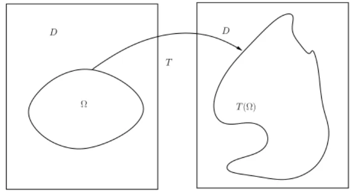
Figure 2.1: Admissible transformationT :D→D
2.3.3 Compositions of Sobolev functions with flows
In the following let θ ∈ Cc1(D,Rd) be a given vector field and Φt = Φθt its associated
flow. Notice that by the chain rule∂Φ−1(t,Φ(t, x)) = (∂Φ(t, x))−1 (briefly (∂(Φ−t1))◦Φt=
(∂Φt)−1 =:∂Φ−t1), which implies3 (∇f)◦Φt=∂Φ−>t ∇(f◦Φt).Throughout this thesis the
following abbreviations are used
ξ(t) := det(∂Φt), A(t) :=ξ(t)∂Φ−t1∂Φ
−>
t , B(t) :=∂Φ
−>
t , (2.6)
where det :Rd,d→ R denotes the determinant. Step-by-step, we will derive properties of the functions ξ,B and A.
Proposition 2.12. Let the mappings A∈C([0, τ];C(D,Rd,d))and ξ ∈C([0, τ];C(D)) be given and assume that A(0) = I and ξ(0) = 1. Then there are constants γ1, γ2, δ1, δ2 >0
and τ >˜ 0 such that
∀ζ ∈Rd, ∀t∈[0,τ˜] : γ1|ζ|2 ≤ζ·A(t)ζ ≤γ2|ζ|2, (a)
δ1≤ξ(t)≤δ2. (b)
Proof. (a) For any t∈[0, τ], we may estimate
|η|2 = (I−A(t))η·η+A(t)η·η
≤ kI−A(t)kC(D,Rd,d)η·η+A(t)η·η.
By continuity of t7→ A(t) there exists for all ε >0, a ˜δ >0 such that for all t∈[0,δ] we˜ have kI−A(t)kC(D,Rd,d) ≤ε.Thus choosing ε= 12, we obtain the desired inequality. Since t7→A(t) is bounded, we also have
A(t)η·η≤ kAkC(D×[0,τ],Rd,d)|η|2 for all t∈[0,τ˜], for all η∈Rd.
(b) It is clear thatξ is bounded in space and time. The inequalities in item (b) follow then from
1 = (1−ξ(t)) +ξ(t)≤ kξ(t)−1kC(D)+ξ(t).
2
3For any scalar functionf∈H1(Rd), we have for allv∈Rdand allx∈D
2.3. Flows, homeomorphism and a version of Nagumo’s theorem 17
Proposition 2.13. Let B : [0, τ]→Rd,dbe a bounded mapping andC >0a constant such that kB−1(t)kL∞(D,Rd,d) ≤ C for all t ∈ [0, τ]. Then for any p ≥ 1 there exist constants C1, C2 >0 such that
∀t∈[0, τ], ∀f ∈Wp1(D) : k∇fkLp(D,Rd) ≤C1kB(t)∇fkLp(D,Rd)
∀t∈[0, τ], ∀f ∈Wp1(D,Rd) : k∂ϕkLp(D,Rd,d) ≤C2kB(t)∂ϕkLp(D,Rd,d). (2.7)
Proof. Estimating
k∇fkLp(D,Rd)=k(B(t))−1B(t)∇fkLp(D,Rd)≤CkB(t)∇fkLp(D,Rd)
gives the first inequality. The proof of (2.7) is similar and omitted. 2
Lemma 2.14. Let θ∈C1([0, τ];Cc1(D,Rd)) be a vector field and Φits flow. The functions
t7→ A(t), t7→ξ(t) and t7→B(t) given by (2.6) are differentiable4 on [0, τ]and satisfy the following ordinary differential equations
B0(t) =−B(t)(∂θt)>B(t) ξ0(t) =tr(∂θtB>(t))ξ(t)
A0(t) =tr(∂θtB>(t))A(t)−B>(t)∂θtA(t)−(B>(t)∂θtA(t))>,
where θt(x) :=θ(t,Φt(x)) and 0:= dtd.
Proof. (i) Let E, F be two Banach spaces. In [8, Satz 7.2, p. 222] it is proved that inv :Lis(E, F)→ L(F, E), A7→A−1
is infinitely times continuously differentiable with derivative ∂inv(A)(B) = −A−1BA−1. Now by the fundamental theorem of calculus, we have
Φt(x) =x+ Z t 0 θ(s,Φs(x))ds ⇒ ∂Φt(x) =I+ Z t 0 ∂θ(s,Φs(x)))ds,
whereI ∈Rd,ddenotes the identity matrix. Thereforet7→∂Φt(x) is differentiable for each
x∈Dwith derivative d
dt(∂Φt(x)) =∂θ
t(x) =∂θ(t,Φ
t(x))∂Φt(x).
Thus if we letE =F = Rd,d and take into account the previous equation, we get by the chain rule
d
dt(inv(∂Φt(x))) =−(∂Φt(x))
−1∂θt(x)(∂Φ
t(x))−1.
(ii) A proof may be found in [97, Prop. 10.6, p. 215].
(iii) Follows from the product rule together with (i) and (ii). 2
4A functionf : [a, b]→R(a, b∈R) is called differentiable if it is differentiable on (a, b) and the right
sided, respectively left sided derivative off exists ina, respectively inb, i.e. (f0)−(a) := limh&0(f(a+h)−
Remark2.15. Note that the first formula can also be derived by differentiating the identity
∂Φt∂Φ−t1 = I, where I is the identity matrix in Rd. That the inverse t 7→ ∂Φ
−1
t is
dif-ferentiable can also be seen by the well known formula∂Φ−t1= (det(∂Φt))−1(cofac(∂Φt))>,
where cofac denotes the cofactor matrix.
Lemma 2.16. Let D⊂Rd be a regular domain and p >1 a real number. Denote byΦt the
flow of θ∈Cc1(D,Rd).
(i) For any f ∈Lp(D), we have
lim
t&0kf◦Φt−fkLp(D)= 0 and tlim&0kf◦Φ
−1
t −fkLp(D)= 0.
(ii) For any f ∈Wp1(D), we have
lim
t&0kf◦Φt−fkW
1
p(D)= 0. (2.10)
(iii) For k∈ {1,2} and any f ∈Wpk(D), we have
lim t&0 f◦Φt−f t − ∇f ·θ Wk−1 p (D) = 0.
(iv) Fixp≥1 and lett→ut: [0, τ]→Wp1(D)be a continuous function in0. Setu:=u0.
Then t7→ut◦Φt: [0, τ]→Wp1(D) is continuous in 0 and
lim
t&0kut◦Φt−ukW
1
p(D)= 0.
Proof. (i) It is proved for instance in [37, p. 529]. (ii) In order to prove (2.16) it is sufficient to show
lim
t&0k∇(f◦Φt−f)kLp(D)= limt&0k∂Φ
>
t((∇f)◦Φt− ∇f)kLp(D)= 0. By the triangle inequality, we have
k∂Φ>t ((∇f)◦Φt− ∇f)kLp(D)≤ k(∇f)◦Φt− ∇f)kLp(D)+k(∂Φt>−I)∇f)kLp(D). For the first term on the right hand side we can use (i) and the second term tends to zero since∂Φ>t →I inC(D;Rd,d).
(iii) A proof can be found in [60, Lem. 3.6, p. 6]. (iv) By the triangle inequality, we get for all t∈[0, τ]
kut◦Φt−ukW1
p(D) ≤ kut◦Φt−u◦ΦtkWp1(D)+ku◦Φt−ukWp1(D).
The last term on the right hand side converges to zero ast&0 due to (ii). For the second inequality note that
kut◦Φt−u◦ΦtkW1 p(D)= Z D ξ−1(t)(|ut−u|p+|B(t)∇(ut−u)|p) 1/p ≤C Z D |ut−u|p+|∇(ut−u)|p 1/p
and the right hand side converges to zero ast&0. 2
2.4. Shape continuity 19
2.4
Shape continuity
In this section, we collect existence results of shape optimization problems for special types of shape functions. In Chapter5these will be applied to obtain existence of optimal shapes for several PDE constrained optimization problems defined on subsets of regular domains D⊂Rd.
2.4.1 Topologies via Lp-metrics
The sets Ξ⊂2Rd respectively Ξ⊂2D (D⊂Rdregular domain) are in general no subsets
of a locally convex vector spaces. Therefore there is no ’canonical’ choice of a topology as it is for functions f : U → R defined on open subsets U of topological vector spaces
X. However, for special classes of shape functions there are natural choices of topologies. One such class consists of shape functions depending on the shape only via a characteristic function, i.e.
J(Ω) = ˆJ(χΩ), for some function ˆJ :Xµ(D)→R, where
Xµ(D) ={χΩ : Ω isµ−measurable subset ofD}
denotes the set of characteristic functions defined byµ-measurable subsets ofD. Here,µis Radon measure, that is, a measure on theσ-algebra of Borel sets ofRdthat is locally finite and inner regular.5 For simplicity, we can think of the Lebesgue measurem in which case we set X(D) := Xm(D). We may equip Xµ(D) with the metric induced by the Lp(D, µ)
norm,p∈[1,∞):
δp,µ(χ1, χ2) :=kχ1−χ2kLp(D,µ).
When µ is the Lebesgue measure m we put δp := δp,µ. Convergence Ωn →Lp,µ Ω, where Ωn,Ω∈Dmeans then limn→∞δp,µ(χΩn, χΩ) = 0.
Remark 2.18. Note that we view µ-measurable subsets Ω⊂D as characteristic functions
χΩ and the latter ones are seen as elements of Lp(D, µ). Therefore we loose information,
because two characteristic functions are equal if they are equalµ-almost everywhere on D. That means two sets are equal if they are equalµ-almost everywhere. This is important to keep in mind when one is interested in cracks.
Proposition 2.19. Then Xµ(D)∩L1(D, µ) is closed in Lp(D, µ) and the metric space
(Xµ(D)∩L1(D, µ), δp,µ) is complete. The topologies generated byδp,µ are equivalent for all
p∈[1,∞).
Thus we get a natural topology on Xµ(D)∩L1(D, µ) induced by the normk · kLp(D,µ) and can speak of the continuity ofχ7→Jˆ(χ).
Unlike normal Lp-spaces for p ∈ (1,∞) the spaces Xµ(D)∩L1(D, µ) are not weakly
closed. This is problematic concerning the existence of optimal solutions of optimization problems, since we would like to extract a converging subsequence of minimizing sequence that converges in the same space. In order to obtain a certain compactness an additional stronger term can be added.
5
2.4.2 Topologies via BV-metric
Characteristic functions are not weakly differentiable since they are discontinuous along hypersurfaces of dimension one below the space dimension. That means a characteristic function defined by a subset of the plane has discontinuities along lines and in the three space it has discontinuities along surfaces. Nevertheless an appropriate notion of weak derivative allows us to talk of derivatives of characteristic functions.
We begin with the definition of this notion of weak derivative.
Definition 2.20. Let D⊂Rd be open. We say that u∈L1(D) is of bounded variation if there exists a vector valued Radon measureµ such that
Z D udiv (ϕ)dx=− Z D ϕ·dµ,
for all ϕ∈Cc1(D,Rd). Then one writes du=µ, that indicates the ’weak derivative’ of u is a vector valued Radon measure. The space of all functionsu∈L1(D)that have a derivative
that is a vector valued Radon measure is denoted by BV(D). It becomes a Banach space when equipped with the norm
kfkBV(D):=kfkL1(D)+Var(f, D), (2.11) where Var(f, D) := sup Z D div (ϕ)χ dx|ϕ∈Cc1(D,Rd),kϕkL∞(D)≤1
denotes the total variation of f with respect toD.
The set of all characteristic functions with finite total variation is denoted by
B(D) :={χ∈X(D) : χ∈BV(D)}. (2.12) We put ˆPD(χ) := Var(χ, D) forχ∈X(D). Now we can say what a set of finite perimeter
is.
Definition 2.21. A subset Ω ⊂ Rd is said to have finite perimeter relative to D ⊂ Rd if PD(Ω) := ˆPD(χΩ) < ∞. If D = Rd then we define Pˆ(χ) := Var(χ,Rd) and P(Ω) :=
ˆ
P(χΩ). In other words, a subset Ω⊂D has finite perimeter if the characteristic function χ=χΩ ∈X(D) belongs to the spaceBV(D).
If Ω ⊂ D, then PD(Ω) = P(Ω). One should keep in mind that a finite perimeter set
Ω ⊂ Rd, that is PD(Ω) < ∞, can have non zero d-dimensional Lebesgue measure, i.e.
m(∂Ω)>0. This is even true for the relative boundary∂Ω∩D; see [48, p. 7]. We have the following compactness result:
Theorem 2.22. Let D ⊂ Rd be a Lipschitz domain. We endow BV(D) with the norm
(2.11). Then the space BV(D) is compactly and continuously embedded into Lq(D), q ∈
[1,d−d1), written
BV(D),→c Lq(D),
that is, the identity operator id : BV(D) → Lq(D) is continuous and compact for each
q∈[1,d−d1).
2.4. Shape continuity 21
Corollary 2.23. Let D⊂Rd be a Lipschitz domain andq ∈[1,d−d1).
(i) The set B(D) is closed in BV(D). For any bounded sequence (χn)n∈N, χn ∈B(D),
there exists a subsequence (χnk)k∈N converging inLq(D) to some characteristic
func-tion χ∈X(D) such that
Var(D, χ)≤lim inf
k→∞ Var(D, χnk)<∞.
(ii) The space B(D) equipped with the metric δBV(χ1, χ2) := kχ1−χ2kBV(D) (χ1, χ2 ∈ BV(D)) is a complete metric space.
Proof. (i) Fix q ∈ [1,d−d1). Let (χn)n∈N, χn ∈ B(D) = X(D)∩BV(D) be any
converging sequence with limit χ∈ B(D)⊂ X(D) (closure and convergence with respect to δBV). Note that the sequence (χn)n∈N is bounded in B(D). Therefore, according to Theorem 2.22, we may extract a subsequence (χnk)k∈N converging in Lq(D) to χ ∈ X(D). We show that Var(·, D) : BV(D) → R is lower semi-continuous with respect to the δ1-topology. Let (un)n∈N be a sequence in BV(D) converging in L1(D) to u ∈ BV(D). Set j := lim infn→∞Var(un, D), then by definition of the lim inf, we may extract
a subsequence of (un)n∈N such thatj= limk→∞Var(unk, D). Then for anyφ∈C 1
c(D,Rd)
withkφkL∞(D)≤1, we have lim inf
n→∞ Var(un, D) = limk→∞Var(unk, D)≥klim→∞
Z D unkdiv (φ)dx = Z D lim k→∞unkdiv (φ)dx = Z D udiv (φ)dx,
where we applied Lebesgue’s dominated convergence theorem Theorem A.7. Since this inequality is true for allφ∈Cc1(D,Rd) withkφkL∞(D) ≤1, we obtain
lim inf
n→∞ Var(un, D)≥Var(u, D).
This shows thatχ∈B(D).
(ii) Since a closed subset of a complete metric space is complete, the result directly follows
from (i). 2
Minimizing in B(D)-spaces is theoretically nice, but for applications may be not the optimal choice. One reason is that B(D) yield a too big class of domains which includes highly irregular domains. The continuity of shape function with respect to this metric is defined as the following.
Definition 2.24. Let D ⊂ Rd be Lebesgue measurable and bounded. We say that Jˆ : B(D) → R is continuous in χ ∈B(D) with respect to the δBV metric if for any sequence
χn∈B(D) converging with respect to this metric to χ, we have
lim
n→∞
ˆ
J(χn) = ˆJ(χ).
The following theorem states the existence of shape optimization problems defined on finite perimeter sets.
Theorem 2.25. Let Jˆ:X(D)→ R be a shape function that is continuous with respect to theδp-metric for some p >1. Assume thatinfχ∈X(D)Jˆ(χ)>−∞. Define for anyα >0the
cost functionJˆ:B(D)→R by Jˆ(χ) := ˆJ(χ) +αPˆD(χ).Then the minimisation problem
inf
χ∈X(D) ˆ
J(χ)
has at least one solution χ∈B(D).
Proof. Set j := infχ∈X(D)Jˆ(χ). By definition we have j ≥ infχ∈X(D)Jˆ(χ) > −∞. Let (χn)n∈N be a minimizing sequence in X(D), such that limn→∞Jˆ(χn) = j. Since
infχ∈X(D)J(χ)ˆ >−∞, there must be a constant c >0 such that
∀n∈N: ˆPD(χn)≤c.
Finally, taking into account Corollary2.23, noting that ˆPD(·) = Var(D,·) :BV(X)→Ris
lower semi-continuous and that ˆJ continuous with respect to the δp-metric, we get
ˆ J(χ)≤ lim n→∞ ˆ J(χn) =j 2 2.4.3 Topologies via Ws p-metrics
Although characteristic functions are not weakly differentiable in general, they can have a finite Gagliardo semi-norm. This leads to the notion of the Gagliardo6 perimeter.
For every p∈(1,∞) and 0< s <∞, the Gagliardo semi-norm is defined by
|u|pWs p(D):= Z D Z D |u(x)−u(y)|p |x−y|d+sp dx dy.
The fractional Sobolev space Wps(D) is defined as the completion of Cc∞(D) with respect to the norm
u7→ kukWs
p(D):=|u|Wps(D)+kukLp(D). It is a reflexive Banach space.
Note that the norms on Wps(D) and Wps00(D) are equivalent if sp = s0p0. Moreover,
notice that for a characteristic function χΩ, Ω⊂ D the norm |χΩ|Ws
p(D) depends only on the value of the space dimensiond≥1 and the productsp∈(0,∞), since
|χΩ|pWs p(D)= Z D Z D |χΩ(x)−χΩ(y)| |x−y|d+sp dx dy. In other words|χΩ|pWs p(D)=|χΩ| p0 Ws0 p0(D)
ifsp=s0p0. This leads to the following definition. Definition 2.26. Let Ω⊂D be Lebesgue measurable and s∈ (0,∞). We say that Ω has finite s-perimeter relatively to D if
Ps(Ω) := Z D Z D |χΩ(x)−χΩ(y)| |x−y|d+s dx dy <∞
We callPDs(Ω)the s-perimeter ofΩrelative toDand putPˆDs(χ) :=RDRD |χΩ(x)−χΩ(y)|
|x−y|d+s dx dy.
6
E. Gagliardo introduced the fractional Sobolev norm to characterise traces. Usually, this norm is referred to as fractional Sobolev norm, but since it was Gagliardo who introduce it we use his name.
2.4. Shape continuity 23
For every ¯s ∈ (0,∞), we define the space of characteristic functions having finite ¯ s-perimeter by
W¯s(D) :={χΩ:R→R|χΩ ∈X(D) and ˆPD¯s(χΩ)<∞}.
Note that for 0 ≤s < 1/p ≤ 1, we have BV(D)∩L∞(D) ⊂ Wps(D), see [37, Thm. 6.9.,
p. 253]. That means for ¯s∈(0,1), we obtainB(D)⊂Ws¯(D) andW¯s(D) =X(D)∩Wps(D), when ¯s:=sp.
Compared with the perimeterPD(Ω) the s-perimeterPDs(Ω) provides a weaker
regulari-sation. In particular, the regularisation term and its shape derivative are domain integrals, but they are non-local. Also note that an open and bounded set Ω ⊂ Rd of class C2 has finite perimeter and thus χΩ ∈ BV(D)∩L∞(D), which implies χΩ ∈ W¯s(D) for all ¯
s∈(0,1).
Let 0≤s <1/p≤1 and ¯s=sp. Then we introduce the metricsδs,p on Ws¯(D) by
δs,p(χΩ1, χΩ2) :=|χΩ1 −χΩ2|Wps(Ω)+kχΩ1 −χΩ2kLp(D).
These metrics are all generating the same topology onW¯s(D).
Theorem 2.27 ([41]). Let D ⊂ Rd be a Lipschitz domain and s ∈ (0,1), p ∈ [1,∞), q ∈
[1, p]. Assume that T is a bounded subset of Wps(D) such that
sup
u∈T
|u|Ws
p(D)<∞.
ThenT is relatively compact in Lq(D).7
Corollary 2.28. Let D ⊂ Rd be a regular domain with boundary Σ = ∂D. Let s¯ ∈
(0,∞), s∈(0,s]¯ and p:= ¯s/s≥1.
(i) The setWs¯(D) is closed inWps(D). For any bounded sequence(χn)n∈N, χn∈W¯s(D),
i.e. PDs¯(χn) =|χn|Ws
p(D) ≤C for all n∈N, where C >0, there exist a subsequence (χnk)k∈N converging in Lq(D) to some characteristic function χ∈X(D) such that
ˆ
PDs¯(χ)≤lim inf
k→∞
ˆ
PDs¯(D, χnk)<∞.
(ii) The space (Ws¯(D), δs,p) is a complete metric space.
Proof. (i) First note that any sequence converging in Ws(D) also converges in X(D) with respect toδ1. Now let (χn)n∈N, χn ∈Ws(D) be any converging sequence with limit
χ ∈ Ws(D) ⊂ X(D) (closure and convergence with respect to δ
BV). We may extract
based on Theorem 2.27 a subsequence (χnk)k∈N converging in Lq(D) to χ ∈ X(D). To finish the prove it is sufficient to show that PDs¯(·) = | · |Ws
p(D) : W
s
p(D) → R is lower
semi-continuous with respect to theδ1-metric. To prove this let (un)n∈N be any sequence inWps(D) converging in L1(D) to u ∈ Wps(D). Set j := lim infn→∞|un|pWs
p(D). Note that by definition of the lim inf, we may extract a subsequence denoted (unk)k∈N such that j= limk→∞|un|Ws
p(D) and a further subsequence still denoted (un)n∈N such that unk → u ask→ ∞ almost everywhere inD. Therefore setting
fn(x, y) := |unk(x)−unk(y)| |x−y|d+sp , f(x, y) := |u(x)−u(y)| |x−y|d+sp , 7
In a topological vector spaceX a subsetAis called pre-compact or relatively compact if the closureA inX is compact.
we get limn→∞fn=f a.e. in D×D.Therefore applying Fatou’s LemmaA.6 yields lim inf n→∞ |un| p Ws p(D)= lim infk→∞ Z D×D |unk(x)−unk(y)| |x−y|d+sp d(x, y) ≥ Z D×D |u(x)−u(y)| |x−y|d+sp d(x, y) =|u|pWs p(D),
whered(x, y) =dx dy is the product measure. This concludes the prove.
(ii) Since a closed subset of a complete metric space is complete, we only need to show that
Ws¯(D) is closed, but this follows directly from (i). 2 The following theorem is the key for shape optimization problems defined on finite Gagliardo perimeter sets.
Theorem 2.29. Let Jˆ:X(D)→ R be a shape function that is continuous with respect to the δp-metric for some p > 1. Assume that infχ∈X(D)J(χ)ˆ >−∞. Define for any α >0
and s∈(0,1) the cost functionJˆ:Ws(D)→R ˆ
J(χ) := ˆJ(χ) +αPˆDs(χ).
Then the minimisation problem
inf
χ∈Ws(D) ˆ
J(χ)
has at least one solution.
Proof. Put j := infχ∈Ws(D)Jˆ(χ). By definition j ≥ infχ∈X(D)J(χ) > −∞. Let (χn)n∈Nbe a minimizing sequence inX(D) such thatj= limn→∞Jˆ(χn). By Corollary2.28
we may extract a subsequence (χnk)k∈N converging Lp(D). Finally, taking into account Corollary2.28 part (i) and that ˆJ(·) is continuous inX(D) with respect to theδp metric,
we obtain ˆ J(χ)≤ lim k→∞ ˆ J(χnk) = inf χ∈Ws(D) ˆ J(χ). 2
2.4.4 Shape continuity via flows
In the next section, we are going to introduce the shape derivative. A feature of a derivative should be that if a function is differentiable then it is continuous with respect to some topology. It is not clear if a shape function is continuous with respect to the previously introduced topologies even if the shape function is shape differentiable. Nevertheless, the following concept of continuity is well-suited.
Definition 2.30. Let X ⊂(Rd)R
d
be a given non-empty set.
(i) We say that a subset Ξ⊂2Rd isX-stable atω0∈ΞifF(ω0)∈Ξfor all F ∈X. This
definition is equivalent toZX,ω0 :={F(ω0)|F ∈X} ⊂Ξ.
(ii) We say that Ξ is weakly flow stable if for every ω0 ∈ Ξ there exists a τ > 0 and
an open, bounded set D ⊃ ω0 such that Φθt(ω0) ∈ Ξ for all t ∈ [0, τ] and all θ ∈
2.5. Sensitivity analysis 25
Note that if Ξ isX-stable at all ω0 ⊂Ξ and id∈X, then necessarily∪ω0∈ΞZX,ω0 = Ξ.
It is clear that if Ξ isX-stable at ω0 then it is also Y-stable at ω0 for any Y ⊂ X. Flow stable subsets of 2Rd are important for the shape continuity along flows.
Example 2.31. Let D⊂Rd be open and bounded. The following sets are flow stable
Ξ1 :={Ω⊂D: Ω is open }
Ξ2 :={Ω⊂D: Ω is closed }
Ξ3 :={Ω⊂D: Ω is open and Lipschitzian}.
Definition 2.32. Let D ⊂Rd be a regular domain. Let J : Ξ → R be a shape function defined on a weakly flow stable subset Ξ ⊂ 2D and Θ be a topological vector subspace of Lip0(D,Rd). We say that a shape functionJ is shape continuous8 atΩ∈ΞonC([0,1],Θ)
if
lim
t&0J(Φ
θ
t(Ω)) =J(Ω) for allθ∈C([0,1],Θ).
We say that J is shape continuous on C([0,1],Θ) if it is shape continuous at all Ω∈Ξon
C([0,1]; Θ). If Θ =Cc∞(D,Rd) then we denote the set of all real valued shape continuous shape functionsJ : Ξ⊂2D →R by CD0(Ξ,R) =CD0(Ξ).
Later in Chapter 6, we introduce metrics on spaces of diffeomorphisms in Rd. Defi-nition 2.32 will give a criterion when a shape function is continuous with respect to this metric.
The existence of minimisers of minimisation problems over flows is redirected to Sub-section6.2.1. It involves more definitions and some basic tools from differential geometry, which will be introduced in Chapter6.
2.5
Sensitivity analysis
TheEulerian semi-derivative of a shape functions Ω7→J(Ω) is similar to the Lie derivative on manifolds. It can be interpreted as a derivative of J with respect to the domain Ω. The shape derivative is then defined as the Eulerian semi-derivative with the additional property that it is continuous and linear with respect to the direction. The vanishing of the shape derivative can be interpreted as a necessary optimality condition, which does not necessarily guarantees that a local minimum is attained.
2.5.1 Eulerian semi-derivative and shape derivative
TheEulerian semi-derivative may be defined in two ways. We first describe what is known in the literature as perturbation of identify. For a fixed set Ω ⊂ D define the family of
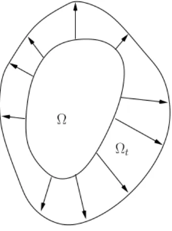
perturbed domains Ωt := (id +t θ)(Ω), where θ ∈ C0,1(D,Rd) with θ = 0 on ∂D and id
denotes the identity mapping onRd. Forτ >0 sufficiently small the mappingx7→Φt(x) :=
x+tθ(x) is invertible9 for each t∈[0, τ]. Then one defines the Eulerian semi-derivative as dIdJ(Ω)[θ] := lim
t&0
J((id +t θ)(Ω))−J(Ω)
t . (2.13)
8In [17, Def. 1, p. 50] this is called directional continuous.
9 LetD⊂Rdbe a regular domain. Pick an elementθ∈C0,1(D) and assume that∂θ(x)<1 atx∈D.
Now since for any matrixA ∈Rd,d the perturbation A+I is invertible if the series P∞
n=1A
n
converges absolutely, in particular ifkAk<1, we get that (I+∂θ(x))−1exists. Thus by the inverse function theorem
we get that (id +θ)−1 exists in (id +θ)(Br(x)) for somer >0. Therefore assumingk∂θkC(D,Rd,d)<1, we
Ω
Ωt
Figure 2.2: Perturbed Ωt and unperturbed domain Ω
The second way to define the Eulerian semi-derivative is referred to as velocity method
or speed method. Instead of considering id +t θ, we replace this function by the flow Φθt generated by a vector field θ belonging to Lip0(D,Rd) and define the Eulerian semi-derivative at Ω in direction θas
dflJ(Ω)[θ] := lim
t&0
J(Φθt(Ω))−J(Ω)
t .
Note that the function Φθ
t := (id +t θ) is the flow of the time-dependent vector field
θ(t) :=θ◦(id +t θ)−1 with supp(θ(t))⊂Dfor each t∈[0, τ]. Thus if (2.13) exists then dIdJ(Ω)[θ] =dflJ(Ω)[θ].
Let Θ⊂Lip0(D,Rd) be a Banach subspace. Then if C([0, τ]; Θ)→ R: ˜θ 7→ dflJ(Ω)[˜θ] is linear and continuous, we conclude by [37, Thm. 3.1, p. 474] that
dflJ(Ω)[θ] =dflJ(Ω)[θ(0)] =dflJ(Ω)[θ]
and thus both derivatives coincide. The following definition is given for autonomous vector fields, but can be immediately extended to the time-dependent case.
Definition 2.33. Let D ⊂ Rd be a regular domain. Let J : Ξ → R be a shape function defined on a flow stable set Ξ ⊂2D and Θ be a topological vector subspace of Cc∞(D,Rd). The Eulerian semi-derivative or Lie semi-derivativeof J atΩin direction θ∈Θ is defined by dJ(Ω)[θ] := lim t&0 Φ∗tJ−J t (Ω), (2.14)
where Φ∗t(f) := f ◦ Φt denotes the pull-back. The semi-derivative is also denoted by Lθ(J)|Ω :=dJ(Ω)[θ].
(i) We call J shape differentiable at Ω with respect to Θ if it has a Eulerian semi-derivative at Ωfor all θ∈Θ and the mapping
θ7→dJ(Ω)[θ] =:G(θ) : Θ→R
is linear and continuous, in which case G(θ) is called the shape derivativeat Ω. (ii) We call J continuously shape differentiable at Ω in Θ if it is shape differentiable at