M. D. Rossetti, R. R. Hill, B. Johansson, A. Dunkin, and R. G. Ingalls, eds.
ANALYZING PRODUCTION MODIFICATIONS OF A C-130 ENGINE REPAIR FACILITY USING SIMULATION
Jeremy D. Jordan Air Force Research Laboratory
Area B, Bldg 190
Wright-Patterson AFB, OH 45433, U.S.A.
Sharif H. Melouk
Department of Information Systems, Statistics, and Management Science, University of Alabama
300 Alston Hall Tuscaloosa, AL 35487, U.S.A. Paul D. Faas
Air Force Research Laboratory Area B, Bldg 190
Wright-Patterson AFB, OH 45433, U.S.A.
ABSTRACT
The LRAFB C-130 engine repair facility is one of the top T-56 engine refurbishing plants in the United States Air Force. Currently, the shop is prevented from testing potential contingencies within their environment due to the rapid nature of their engine repair process. A simulation approach is needed to test various scenarios and determine the maximum capacity the shop can handle in its current configuration. Particularly, the simulation describes the consequences of increasing engine production on the shops personnel and throughput production figures for several policy variations. A detailed verification and validation of the model are shown, establishing the computational efficacy of the model in preparation for the comparative analysis. The model is a starting block for an Air Force wide analysis of C-130 engine rebuilding production needs with an overarching goal of standardization in repair methods and efficient operations.
1 INTRODUCTION
The Air Force currently operates many C-130 level III maintenance shops around the world and is considering merging these into a number of major shops, with the Little Rock Air Force Base (LRAFB) Engine Regional Repair Center (ERRC) being one of the lead engine maintenance shops in the Air Force (AF). The average cost to rebuild an engine at the ERRC is quite high. Testing various scenarios and configurations would be extremely costly because many engines are needed to answer the types of questions posed by decision makers. Thus a discrete event simulation was constructed to represent the system for the purpose of studying and analyzing it. While it may be possible to set up a model that can be solved analytically, simulation provides the most convenient and efficient means of representing the system. Since the shop is a conglomeration of stochastic relationships, the simplifying assumptions needed to build a mathematical model of this type would likely render the analysis inadequate. The simulation approach allowed great flexibility in representing the real system, and allowed the testing of different policies, varying parameters, alternate designs, and contingency scenarios. This was the first application of operations research in the shop.
The C-130 facility’s management historically used Lean Thinking to determine improved configurations for the shop, however this is not without its deficiencies as noted in Standridge and Marvel (2006). There are obvious parallels between Lean Manufacturing techniques and Operations Research principles, however practitioners from the two disciplines are often in conflict. OR proponents deem Lean as lacking in mathematical rigor, while Lean labels OR as far too complex for practical applications. This is discouraging as there are several overlaps that should taken advantage of. For instance, in addition to the common sense fostered by Lean Thinking, simulation allows modeling and assessing the effects of variation, making use of all available data, validating effects of possible changes before implementing, and determining interaction effects between variables in the system. Others, such as Detty and Yingling (2000), use discrete event simulation to show
the benefits of implementing lean thinking. Lean recommendations are initiated in the simulation and compared against the baseline operations, thus providing foresight in the form of efficiency increase predictions. Essentially, any business that has implemented lean manufacturing while ignoring discrete event simulation is ripe for action. These businesses typically have all the necessary data for an analyst to swiftly construct and validate a simulation. Much of the data used for simulation is used for lean manufacturing as well. To implement one of these techniques devoid of the other is inefficient and wasteful, the two reasons both of these techniques were developed. Consequently, lean ”experts” in the shop were a hard sell, stating that simulation provides little benefit in a process oriented production environment. Nonetheless, the data collected by the C-130 engine shop AFSO21/Lean team for lean practices purposes was used to populate this simulation, thus minimal data collection was necessary.
Hoffer, Haar, and Hagerman (2008) discuss the application of the key principles of Lean manufacturing in the ERRC. Production efficiency in the shop increased 30 percent during the 2 year period from 2006-2008. The specific improvements outlined in the paper have increased excellence in the shop, however this simulation study provides an opportunity to enhance and broaden the scope of change. The objectives and purpose of this research are as follows:
• Model the flow of engines, employee schedules, and service times required to complete various processes. • Determine the monthly capacity of engine production the ERRC can handle in its current configuration. • Determine manpower needs and possible areas for improvement.
Accomplishing these objectives allows us to answer questions such as the following: • What is the maximum throughput of the ERRC in its current configuration? • What are the impacts of increasing workload on the system?
• What effects will greater production demands have on the system and manpower? • What are the long term effects of increasing throughput?
The steps taken in this study mimic standard simulation procedures from textbooks. For a thorough description of simulation techniques, we refer to Banks (2005) and Law and Kelton (2000). In reviewing parts of the literature and through regular contact with novice modelers, parts of these steps are often circumvented. The most notable mistakes include unclear problem definitions or model purposes that match up poorly with the model conceptualization. Additionally, severely truncated verification and validation practices are quite common and preferred by many. One of the contributions of this paper is an example of how to properly perform a simulation study with a military simulation problem. The paper clearly defines our purpose and demonstrates a practical application of basic verification and validation techniques.
There are numerous studies applying discrete event simulation to maintenance and production activities, yet the application in this paper is unique and distinctive insights can be gained. Gatland, Yang, and Buxton (1997) look at the simulation of a delta engine repair shop to solve engine maintenance capacity. They consider all parts of an aircraft and the ensuing repair personnel. We focus on an engine tear-down and buildup. Park, Matson, and Miller (1998) examine a Mercedes Benz production facility, examining the three components being the body shop, the paint shop, and the assembly shop. The study shows the shop is not capable of producing the required 270 engines per day. Our study provides similar insight into the capacity of the engine shop in its current configuration yet includes further technical detail.
The engines in this study are disassembled and reassembled through three main processes in the engine shop. We name these main process 1, 2, and 3 for simplicity. Main process 1 is the primary tear down and buildup procedure, main process 2 refurbishes the various parts of the T-56 engine, and main process 3 refurbishes the outer casing of the engine. Section 2 looks at a detailed description of the engine shop and the modeling process. Section 3 shows verification and validation applications and results from runs of the simulation. Section 4 lays out our concluding comments and practical implications for the engine shop and the Air Force.
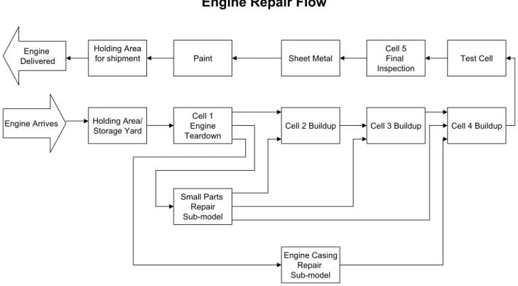
2 PROBLEM DEFINITION 2.1 System Structure
The essence of the real system is captured through a high level view of the engine shop as shown in Figure 1. Initially, an engine arrives for repair and is accepted into the storage yard. It waits in the storage yard until selected to be rebuilt at which point it actually enters the engine shop. The engine is broken down to its base structure in Cell 1 and sent to the three different main processes. The various parts are sent to the parts repair sub-model (main process 2), where each part
is refurbished or replaced through a number of processes. The QEC or engine housing is sent to the engine housing repair sub-model (main process 3) and further broken down to allow for full repair. The baseplate containing the serial number of the original engine is sent to Cell 2 (main process 1) for initialization of the engine rebuild. Interesting to note, the new engine being constructed actually uses parts from previous engines that have been torn down and uses none of its original parts. The parts flow through the parts repair sub-model and are stored in containers until needed in Cells 2 and 3, the main buildup cells. The engine housing is repaired through its sub-processes and sent to Cell 4 for installation. Engine testing is initiated in Cell 5 following successful buildup in the previous three cells. Once operational capability testing metrics are satisfactory, the engine progresses into the final inspection cell. Painting and shipment to the customer occur following successful testing. In addition to the processes in Figure 1, there are many sub-processes within each of the processes. Rather than make a common mistake to model fastidiously with excessive fidelity, we chose to keep the model at this level in order to complete our objectives outlined above. This common blunder of attempting to capture every detail within a system can often times be traced back to the purpose of the model. In many cases, the purpose of the model is not well defined which leads to impulsive, unstructured modeling. If in the future the shop decides it needs a different set of answers, such that the model must capture all the detailed sub-processes, the current model can be easily expanded to satisfy any modifications to the purpose of the model.
Engine Repair Flow
Engine Arrives Holding Area/
Storage Yard Cell 3 Buildup
Small Parts Repair Sub-model Engine Casing Repair Sub-model Cell 4 Buildup Cell 1 Engine Teardown Cell 2 Buildup Test Cell Holding Area
for shipment Paint Sheet Metal
Cell 5 Final Inspection Engine
Delivered
2.2 System Model Design
The above system was modeled using the discrete-event modeling software Arena. Engine arrivals to the shop were based on a schedule of 7 per month, the current Air Force demand of this specific shop. Engines departed the storage yard holding area following successful teardown of the previous engine in Cell 1 as shown in Figure 1. Resource levels were setup using the schedule function, assigning 17 resources to 8 hour shifts from 8AM to 4PM. Following entrance into the physical facility, the engine undergoes teardown in Cell 1, represented by an empirical distribution. It was necessary to define the majority of the processes using empirical distributions since most processes failed the goodness of fit statistical tests i.e. Kolmogorov-Smirnov and Chi-Square. Since over 100 data points existed for the length of time that each of the processes described above took to complete, these were used to assign a random length of time needed to accomplish the process. In a few cases, distributions such as the weibull and gamma fit nicely to the process. Following successful teardown in Cell 1, the engine entity is duplicated and assigned attributes to describe their new identity, i.e. baseplate, engine parts, housing. Each of the entities are then sent to their respective sub-models as described in the previous section. Each of the entities are then serviced by the sub-models, and are subsequently injected back into the main process to be matched up with entities of the other 2 types. The engines are finally painted and sent through the sheet metal process to be disposed. Next, we verify and validate the model to be used for analysis purposes.
3 RESULTS
With a well defined purpose and structure, it follows that verification and validation techniques be performed and results be extracted accordingly. This simulation is useful for answering many questions, initially for the ERRC alone. It also provides a framework for a fleet-wide analysis of C-130 engine needs in the Air Force. The idea is to replicate the LRAFB ERRC across the Air Force in order to ensure standardization in repair methods and efficient operations. Initially, we utilize the simulation to provide the capacity or throughput of the shop, determine effects of varying levels of capacity on manpower, and compare different scenarios that may occur in the shop. To decipher whether or not the results of the model are truly useful, an examination of the techniques used for verification and validation must transpire. Following this, we attempt to answer the questions posed above with the model.
3.1 Verification and Validation
Along with the every growing rapid acquisition of information capabilities of the present age come unrealistic expectations from simulation practitioners in the form of immediate answers to decision maker questions. The proper practices of simulation have been in a downward spiral for many reasons, including the easy attainment and ease of building models in object oriented simulation software. This problem is not necessarily among the academic community, but more so with amateur analysts who hastily construct models. Discussions with modelers have revealed confessions of sweeping V&V under the rug, dismissing its importance in the overall project details. Through interactions with beginner and infrequent modelers, several reasons have emerged:
1. V&V takes time Decision makers are typically impatient when their question lingers to long in the quantitative analysis stage. This leads the modeler/analyst to neglect the proper V&V practice in order to satisfy the time constraints imposed by persons in power.
2. V&V can be difficult V&V is not a trivial step in the model building process. It’s easy for an inexperienced analyst to purchase Arena and build a working model quickly. Completing an adequate V&V of this model increases the necessary skill set, to include people skills for verification and a knowledge of statistics for validation.
3. V&V can add complexity A properly conducted V&V will generally introduce rework into the model building process. It reveals errors that must be dealt with in order to make a valid model.
4. V&V increases costs The cost of validating a model is commonly pricey and increases significantly as the level of confidence required increases.
5. V&V requires data Suitably executing the validation process requires real system performance data to compare against the models output, this can be difficult to obtain in many cases.
Nevertheless, to ensure the model depicts the system accurately, the simulation must be verified and statistically validated. Verification procedures are subjective in nature, and ensure the model is built correctly, representing the input and structure
of the true system. The subject matter experts in the shop examined the model and verified correct operation and structure of the model. In addition, the data input was verified by shop personnel and checked for accuracy by the modelers. Often overlooked is the informal process of examining the model output for reasonableness under a variety of input parameter settings. Varying the incoming number of engines results in an increased wait time for the engines at the various processes, while decreasing the capacity eliminates any time the engines spend waiting for action. A decrease in the number of personnel available for work also results in increased wait times as expected. Additionally, throughout the simulation building process, subject matter experts were engaged thus giving the model a high face validity. High face validity is especially important to ensure the customer feels confident about the tool they will be using and trusting.
Given the various input factors from Section 2, the verified model can now be thought of as a black box. These input factors produce outputs that must be statistically validated, another concept often overlooked by modelers. The outputs produced by the simulation are compared to the true outputs of the engine shop through simple statistical tests as shown in Table 1. The output parameters are designated as follows:
ω, Total Time; ψ, Value Added Time; ρ, Utilization Rate.
Table 1: Validation
Actual System Simulation Output ε Lower 99% CI Upper 99% CI
E[ω] 20.49 20.39 1 20.33 20.45
E[ψ] 17.89 18.77 1 18.72 18.82
E[ρ] .59 .52 .10 .51 .53
Table 1 shows the expected value from the actual system, the expected value of the simulation, the user defined value of ε (1 day), the upper 99% confidence interval and the lower 99% confidence interval, respectively. Through consultation with personnel, we determined that the difference between the simulation model and the actual system should be within the values ofε in Table 1. A few examples of the parameters from the simulation used to validate the model are the average total time spent in repair by each engine E[ω], the average value added time employees spent actually performing work on the engine E[ψ], and the average utilization rate of the employees E[ρ]. The t statistic for the differences between these parameters from the simulation output and the actual system were all well below the critical t value of 2.76. In addition to the parameters we used, the modeler could use values such as work in progress, wait time, or any other collected data from the simulation. We conclude that a difference between the simulation and the actual process does not exist. For an expository treatment of verification and validation techniques and procedures, see Sargent (2008) and Law (2008).
3.2 Comparative Analysis
One of the most powerful traits of a simulation are its comparative capabilities. All simulations imperfectly represent the systems they are attempting to mimic as Box and Draper (1987) state, ”essentially, all models are wrong, but some are useful”. The implications reduce the burden on the model-builder as a model can only be prepared and perfected to a finite point. The desire to construct a perfect model can unnecessarily drive the modeler to spend excessive amounts of time on a model with only marginal benefits. The costs of refining a model begin to outweigh the benefits at some point. Therefore, comparing configurations and scenarios becomes one of the more useful aspects of simulation. This section compares varying levels of factors such as manpower and demand.
Unless otherwise noted, all comparisons assume 3 year time periods with 30 replications. Of course, steady-state parameters were collected for each of the scenarios as well to ensure feasibility, however most of the interesting changes were captured within a 3-year time frame. The shop currently produces 7 engines per month, however this value changes periodically. In addition, the shop undergoes process changes and manpower fluctuations occasionally, thus the 3-year time period provides ample time to evaluate. Varying levels of attempted engine production is shown in Table 2. An increase of 3 engines per month is entirely within the scope of the current configuration and manpower levels of the engine shop. The total average time the engine waits for service across all the processes and the maximum observed number of engines being serviced in the shop increase slightly, but the process remains manageable. Increasing the demand to 13 results in excessive average wait times, the engines will wait at each of the processes for some amount of time before commencing repair. The maximum total number in service exceeds the physical capacity of the shop as the shop does not have enough
room to store and repair 39 engines at one time.
Table 2: Comparison of Varying Levels of Demand
Demand→ 7 per month 10 per month 13 per month Average Value Added Time (days) 18.77 18.82 18.80 Average Engine Wait Time (days) 1.62 3.17 20.35 Average Total Time in System (days) 20.39 21.99 39.15 Maximum Wait Time (days) 12.17 20.28 116.18
Maximum Number in Service 10 13 39
Average Worker Utilization Rate .52 .74 .95 Average Total Engines Produced 258 365 466
Simulation provided the shop a benefit of replicating the engine repair process for long periods of time. Simulation modelers are avidly aware of this important quality, however many managers fail to understand the nature of stochastic processes. Some believe an adequate method for testing a specific scenario is to try out the scenario for a short time. Assume to determine the effects of varying levels of throughput, the engine shop decided to forego simulation for real-world trial and error experimentation. Without a healthy understanding of stochastic principles, a shop analyst may attempt to increase the production levels for a 30-day period and examine the effects on worker utilization, engine wait time (amount of time the engine waited for someone to be available to work on it), and total number of engines produced. From this single experiment, an analyst would extrapolate information to predict the effects for the next several years. Table 3 shows this concept using the same shop configuration as was used to calculate Table 2. Let’s assume the output data in Table 3 is equivalent to a 30 day period on the actual shop floor. Compare the values of Table 3 and Table 2 and notice the distinctive characteristics of the simulation that is replicated many times and run for a long period of time. The value added time and worker utilization rate is relatively similar to the 3-year simulation in Table 2. Notice the average engine wait time and total time in system are not representative of what would truly happen over a 3-year period. Also, the maximum wait time and maximum number in service do not match up with the 3-year simulation numbers. What does this mean? If this approach was taken, the shop managers would incorrectly conclude that their shop is capable of producing 13 engines per month. Rather, excessive wait times causing backups in excess of the physical space available would occur. This shows the benefit of creating a simulation to help answer those questions that cannot be answered through actual experiments in the shop.
Table 3: 1 replication of 30 day scenario in days
7 per month 10 per month 13 per month Average Value Added Time 20.04 17.74 18.47
Average Engine Wait Time 1.28 2.71 7.83 Total Time in System 21.32 20.45 26.30
Maximum Number in Service 8 9 15
Max Wait Time 2.45 3.72 13.04
Worker Utilization Rate .49 .68 .93
Total Engines Produced 7 10 13
Total Engines Produced in 3 Years 252 360 468
Finally we investigate manpower pertubations assuming a static demand of seven engines a month. Although the simulation was not populated for a comprehensive manpower study, practical observations remain viable. For instance, Table 4 shows the effects of varying levels of manpower on the simulation. In all cases the number of engines produced remains the same as with full manpower, that is 17 employees in main process 1. A higher max wait time is still present under each of the cases, but overall the system can adjust to keep the overall average wait time relatively low. Notice the utilization rate obviously increases as less people are available to work. The simulation shows that a reduction in manpower is definitely attainable, yet this is not a prescription to reduce personnel levels. Other factors must be considered such as the amount of additional duties, vacation time, and other intangible factors. The simulation is then a starting point revealing an area that may require further consideration.
Table 4: Manpower
12 13 14 Baseline (17) Average Value Added Time 18.76 18.81 18.78 18.77
Average Engine Wait Time 2.91 2.17 1.75 1.62 Total Time in System 21.32 20.98 20.53 20.39
Max Wait Time 24.80 36.18 16.02 12.17 Worker Utilization Rate .74 .68 .63 .52
4 CONCLUSION
This simulation is useful for answering questions beyond those answered in this paper. It stands as a baseline model to be utilized as shown above, primarily for capacity and comparative purposes. Two additional future directions include breaking down each of the processes into its sub-processes and optimization of manpower schedules. This would allow the shop to determine if the order and placement of their manpower and processes could be improved and optimized. Each process described in this paper takes between 1 and 3 days to complete, however through Lean data collection, each process is further broken down into hundreds of sub-processes. Spending time perfecting the manpower schedule and capturing each of these sub-processes opens the door to use Lean practices on the simulation to a priori determine the effects of implementation possibilities. One of the likely follow ups to this simulation include the replication and slight modification in order to represent all engine repair shops across the AF. This would permit analysis to determine the effects of surges in C-130 aircraft engine needs on the AF and its resources, perhaps during a time of conflict for instance. Additionally, this allows decision makers to see the big picture and possibly conjoin certain shops, shift manufacturing responsibilities to under-utilized shops, and examine a multitude of various policy decisions.
REFERENCES
Banks, J., J.S. Carson II, B.L. Nelson, and D. Nicol. 2005. Discrete-Event System Simulation. 4th ed. Englewood Clifs, NJ: Prentice-Hall.
Box, G.E. and N.R. Draper. 1987. Empirical Model-Building and Response Surfaces. Wiley. p 424.
Detty, R.B. and J.C. Yingling. 2000. Quantifying benefits of conversion to lean manufacturing with discrete event simulation: a case study. International Journal of Production Research38(2): 429-445.
Gatland, R., E. Yang and K. Buxton. 1997. Solving Engine Maintenance Capacity Problems with Simulation. InProceedings of the 1997 Winter Simulation Conference, ed. S.G. Henderson, B. Biller, M. Hsieh, J. Shortle, J.D. Tew, R.R. Barton, 892-899. Piscataway, New Jersey: Institute of Electrical and Electronics Engineers, Inc.
Goldsman, D. and K. Kang. 2002. Simulation of Transportation Logistics. InProceedings of the 2002 Winter Simulation Conference, ed. E. Yucesan, C.H. Chen, J.L. Snowdon and J.M. Charnes, 901-904. Piscataway, New Jersey: Institute of Electrical and Electronics Engineers, Inc.
Hoffer, J., D. Haar and N. Hagerman. 2008. T56 Engine Line-Little Rock AFB Successes and Challenges. Air Force Journal of Logistics32(2): 38-45.
Kuhl, M., J. Kistner, K. Costantini and M. Sudit. 2007. Cyber Attack Modeling and Simulation for Network Security Analysis. In Proceedings of the 2007 Winter Simulation Conference, ed. S.G. Henderson, B. Biller, M.H. Hsieh, J. Shortle, J.D. Tew and R.R. Barton, 1180-1188. Piscataway, New Jersey: Institute of Electrical and Electronics Engineers, Inc.
Law, A.M. and W.D. Kelton. 2000. Simulation Modeling and Analysis. 3rd ed., McGraw-Hill.
Law, A.M. 2008. How to Build Valid and Credible Simulation Models. In Proceedings of the 2008 Winter Simulation Conference, ed. S.J. Mason, R.R. Hill, L. Monch, O. Rose, T. Jefferson, J.W. Fowler, 39-47. Piscataway, New Jersey: Institute of Electrical and Electronics Engineers, Inc.
Painter, M., M. Erraguntla, G.L. Hogg and B. Beachkofski. 2006. Using Simulation, Data Mining, and Knowledge Discovery Techniques for Optimized Aircraft Engine Fleet Management. InProceedings of the 2006 Winter Simulation Conference, ed. L.F. Perrone, F.P. Wieland, J. Liu, B.G. Lawson, D.M. Nicol and R.M. Fujimoto, 1253-1260. Piscataway, New Jersey: Institute of Electrical and Electronics Engineers, Inc.
Park, Y.H., J.E. Matson and D.M. Miller. 1998. Simulation and Analysis of the Mercedes-Benz All Activity Vehicle(AAV) Production Facility. In Proceedings of the 1998 Winter Simulation Conference, ed. D.J. Medeiros, E.F. Watson, J.S. Carson and M.S. Manivannan. Piscataway, New Jersey: Institute of Electrical and Electronics Engineers, Inc.
Sargent, R.G. 2008. Verification and Validation of Simulation Models. In Proceedings of the 2008 Winter Simulation Conference, ed. S.J. Mason, R.R. Hill, L. Monch, O. Rose, T. Jefferson, J.W. Fowler, 157-169. Piscataway, New Jersey: Institute of Electrical and Electronics Engineers, Inc.
Standridge, C. and J. Marvel. 2006. Why Lean Needs Simulation. InProceedings of the 2006 Winter Simulation Conference, ed. L.F. Perrone, F.P. Wieland, J. Liu, B.G. Lawson, D.M. Nicol and R.M. Fujimoto, 1907-1913. Piscataway, New Jersey: Institute of Electrical and Electronics Engineers, Inc.
Thavamani, S. 2006. Control of C2 Unit Using ARENA Modeling and Simulation. In Proceedings of the 2006 Winter Simulation Conference, ed. L.F. Perrone, F.P. Wieland, J. Liu, B.G. Lawson, D.M. Nicol and R.M. Fujimoto, 1316-1323. Piscataway, New Jersey: Institute of Electrical and Electronics Engineers, Inc.
Winston, W. L. 2004. Operations Research: Applications and Algorithms. Thomson Learning.
AUTHOR BIOGRAPHIES
JEREMY D. JORDANis an operations research analyst and Captain in the United States Air Force currently pursuing his PhD in Operations Research from the Air Force Institute of Technology in Dayton, OH. He received his M.S. in Operations Research from the Air Force Institute of Technology in 2007. His research interests include applied statistics, experimental design and simulation. He can be reached by emailing<[email protected]>.
SHARIF H. MELOUK is an operations management professor at the University of Alabama. He received a Ph.D. in industrial engineering from Texas A&M University. His research interests include simulation optimization, discrete-event simulation, and distributed simulation as applied to transportation, homeland security, healthcare, and production/operations. He can be reached by emailing<[email protected]>.
PAUL D. FAASgraduated from Purdue University with a Bachelor of Science in Aeronautical and Astronautical Engineering in 1982. He graduated from the Air Force Institute of Technology with a Master of Science in 2003 majoring in Operations Research. He works for the Sensemaking and Organizational Effectiveness branch in the Air Force Research Laboratory at Wright-Patterson AFB, Ohio. His email address is<[email protected]>.