Tree Data Decision Diagrams
Jean-Michel COUVREUR, Duy-Tung NGUYEN LIFO (Laboratoire d’Informatique Fondamentale d’Orl ´eans),
University of Orleans,
L ´eonard de Vinci street B.P. 6759, F-45067 ORLEANS Cedex 2 http://www.univ-orleans.fr/lifo/
Abstract
In this paper, we present Tree Data Decision Diagrams, a compact data structure of symbolic verification based on term rewriting systems. By this way, we can benefit termination researches in term rewriting systems to improve the model-checking quality. Our experimental implementation uses tree automata technique that provides the capability to maintain the internal representation of data in canonical form.
Keywords: Modelling, model-checking, term rewriting system, symbolic verification, data decision diagrams, termination, tree automata
1. INTRODUCTION
Tree Data Decision Diagrams (TDDD for short) is a hierarchical version of Data Decision Diagrams (DDD) [2, 3] developed in the spirit of the well-known Binary Decision Diagram (BDD) [1].
DDD are a directed acyclic graph structure that manipulates (a priori unbounded) integer domain variables, and which offers a flexible and compositional definition of operations through inductive homomorphisms. In [4], we presented data structure called Set Decision Diagrams (SDD), as an arc of the structure is labeled by a set of values, instead of a single valuation. The set is itself represented by a SDD or DDD, thus in effect we label the arcs of our structure with references to SDD or DDD, introducing hierarchy in the data structure.
TDDD likes DDD structures with representing sets of sequences of assignments of the variables and their values, but each variable has either a value or a sub sequence.
Considering TDDD in term rewriting systems (TRS for short) will be not only compact as SDD (more than DDD) but its operators are also very simpler and more flexibly than the others (more detail in section 3).
Moreover, the two basic techniques used for proving TDDD termination are path orders and semantic labelling. Path orders are direct techniques to prove termination, while semantic labelling is technique for transforming a TRS to another one in such a way that termination of the original TRS can be concluded from (relative) termination of the transformed TRS. For further details we refer to [8, 9, 11, 12].
When a model is proved terminating, we call it a well-designed. Consequently, model designed by TRS can detect the non-terminating component and help developers get oriented to the better designed. When a model is well-designed, the model-checker will generate all of reachability states if the system resources are enough.
At the end of this paper, we report on our experience of implementations using tree automata technique [13] that provides the capability to maintain the internal representation of data in canonical form.
2. PRELIMINARIES
2.1. Term rewriting systems and termination proving
Term rewriting systems. A signature is a countable setFof function symbols (or operators). Associated with every f ∈F is a natural number denoting its arity. Function symbols of arity 0 are called constants. LetT(F, V)be the set of all terms built fromF and a countably infinite setV of variables, disjoint fromF. Iftis a term thenV ar(t)denotes the set of variables occurring int. A termtis called ground ifV ar(t) = ∅. The set of all ground terms is denoted by
T(F). A termtis called linear if it does not contain multiple occurrences of the same variable. The root symbol of a termtis defined as follows:root(t) = tiftis a variable androot(t) =f ift=f(t1, ..., tn). The size|t|of a termtis
the number of variables and function symbols occurring int.
We introduce a fresh constant symbol2, named hole. A contextCis a term inT(F∪ {2}, V). The designation term is restricted to members ofT(F, V). A context may contain zero, one or more holes. IfC is a context withnholes andt1, ..., tn are terms thenC[t1, ..., tn]denotes the result of replacing from left to right the holes inCbyt1, ..., tn. A
termsis a sub-term of a termtif there exists a contextCsuch thatt=C[s]. A sub-termsoftis proper, denoted by t . s, ifs6=t. A substitution is a mapσfromV toT(F, V). Ifσis a substitution andta term thentσdenotes the result of applyingσto t. We calltσan instance of t. A binary relationÂon terms is a rewrite relation if it is closed under contexts and substitutions, i.e. iftÂsthenC[tσ]ÂC[sσ]for all contextsC(with precisely one hole) and substitutions σ.
A rewrite rule is a pair(l, r)of terms such that the left-hand side (lhs)l is not a variable and variables which occur in the right-hand side (rhs)roccur also in l, i.e.V ar(r) ⊆V ar(l). Rewrite rules(l, r)will henceforth be written as l → r. A rewrite rule is collapsing if its rhs is a single variable. A rewrite rule is duplicating if its rhs contains more occurrences of some variable than its lhs. A rewrite rule is left-linear (right-linear) if its lhs (rhs) is a linear term. A TRS is a pair< F, R >consisting of a signature F and a set R of rewrite rules between terms in T (F, V). If(F, R)is a TRS then→Rdenotes the smallest rewrite relation onT(F, V)containing R. Sot→Rsif there exists a rewrite rule l→rin R, a substitutionσand a contextCsuch thatt=C[lσ]ands=C[rσ]. The sub-termlσoftis called a redex and we say thattrewrites tosby contracting redexlσ. We callt→R sa rewrite or reduction step. If C =2then we speak of a root reduction. The transitive closure of→ Ris denoted by→+R and→∗
Rdenotes the transitive-reflexive
closure of R. Ift→∗
Rswe say thattreduces tos.
Termination proving. Termination of TRS is an undecidable problem even with finite< F, R >.
A rewrite relation that is also a (strict) partial order is called a rewrite order. An orderÂis called well-founded if there is no infinite descending sequencet1Ât2Â....
An order onT(F) is called monotonic ift  u ⇒ f(..., t, ...)  f(..., u, ...) for allf ∈ F. A TRS < F, R >and an orderÂare called compatible if t  ufor all rewrite stepst →R u. For compatibility with a monotonic order it suffices to check that lσ  rσ for all rules l → r inR and all ground substitution σ. It is well-known that a TRS is terminating iff it is compatible with some monotonic well-founded order. An orderÂonT(F)is said to have the sub-term property iff(..., t, ...)Âtfor allf ∈F andt∈T(F). The monotonic order satisfying the sub-term property is called a simplification order. A direct consequence of Kruskal’s theorem [8] is that any simplification order over a finite signature is well-founded.
A TRS< F, R >is compatible with a rewrite orderÂonT(F, V)iflÂrfor every rewrite rulel→rof R. It is easy to show that a TRS is terminating if and only if it is compatible with a well-founded rewrite order. The simplification is as the following:
• A simplification order is a rewrite orderÂwith the sub-term property, i.e.C[t]Âtfor all contextsC 6=2(with precisely one hole) and termst.
• A TRS is called simplifying if it is compatible with a simplification order.
• A TRS is called simply terminating if it is compatible with a well-founded simplification order.
Clearly every simply terminating TRS is both simplifying and terminating. A simplifying TRS(F, R)withForRfinite is simply terminating, as a consequence of Kruskal’s Tree Theorem [8]. There exists (infinite) simplifying and terminating TRSs that are not simply terminating, see [10]. This does not concern us too much as we will deal with decidability issues in the sequel, in which one considers only finite (both with respect to signature and set of rewrite rules) TRSs. The recursive path order (RPO) is introduced by Dershowitz. Kamin and Levy present the lexicographic path order (LPO), a well-known variant of the RPO. They are defined recursively as follows:
LetÀbe any order on the signature F. Then for two ground termst = f(t1, ..., tn)andu =g(u1, ..., um)one has
tÂuiff:
• ti=uortiÂufor somei= 1, ..., n,or • f ÀgandtÂuifor alli= 1, ..., m,or
• f =gand{t1, ..., tn} Âmulrpo {u1, ..., um}with RPO
(or(t1, ..., tn)Âlexlpo (u1, ..., um)with LPO).
Here for any order  the order Âlex means the lexicographic extension of  to sequences. The lexicographic
comparison has to be done in a fixed direction; in the paper it will be from right to left. It should be noted that only sequences of equal length are compared, since they require that every symbol has a fixed arity. It is well-known thatÂlpois monotonic and has the sub-term property. FurtherÂlpois total on ground terms iffÀis total onF. Semantic labelling provides a technique for proving termination, making classical techniques like path orders applicable even for non-simplifying TRS’s. LetM be a model for a TRS R over F. Choose for everyf ∈ F a non empty setSf of labels and a mapπf :Mn −→Sf, wherenis the arity off. So TRS< F, R >can be terminating if
the< Flab, Rlab>is terminating.
2.2. Non-deterministic Top-down finite tree automaton
A Non-deterministic Top-down finite tree automaton [13] (NFTA for short) overF is a tupleA = (Q, F, I,4)where Qis a set of states (states are unary symbols),I ⊆Qis a set of initial states, and4is a set of rewrite rules of the following type:
q(f(t1, ..., tn))−→f(q1(t1), ..., qn(tn)),
wheren≥0, f ∈F, q, q1, ..., qn∈Q, t1, ..., tn∈T.
Whenn = 0, i.e. when the symbol is a constant symbolc, a transition rule of NFTA is of the formq(c) −→ c. For simplifying the automata representation, we can name the state¯c∈Qfor each corresponding constant symbolc. Ex:
¯1(1)−→1or¯$($)−→$.
An automaton starts at the root and moves downward, associating along a run a state with each sub-term inductively. The tree languageL(A)recognized byAis the set of all ground termstfor which there is an initial stateqinI such thatq(t)−→∗
At.
We can organize data structure for finite tree automaton (i.e. no cycle exists in the tree automaton) with respecting the canonicity. It should be noted that a canonical finite tree automaton has not always a minimal state number. In infinite case, we must use minimization algorithm for Non-deterministic tree automaton like bisimulation minimization [14, 15], etc.
2.3. Data Decision Diagrams and Set Decision Diagrams
Data Decision Diagrams [2, 3] are a directed acyclic graph structure that manipulates (a priori unbounded) integer domain variables, and which offers a flexible and compositional definition of operations through inductive homomorphisms.
DDD are data structure for representing finite sets of assignments sequences of the forme1 −→x1 e2 −→x2 ...en −−→xn 1
whereei are variables andxi are the assigned integer values. When an ordering on the variables is fixed and the
values are boolean, DDD coincides with the well-known Binary Decision Diagram. However DDD assume no variable ordering and, even more, the same variable may occur many times in the same assignment sequence. Moreover, variables are not assumed to be part of all paths. Therefore, the maximal length of a sequence is not fixed, and sequences of different lengths can coexist in a DDD. This feature is very useful when dealing with dynamic structures like queues.
Operators on these structures are not hard-coded, but a class of operators, called homomorphisms, is introduced to allow transition rules coding. A special kind of homomorphisms uses only local information to a node in its definition. Together with composition, concatenation, union, etc operations, general homomorphisms are defined.
DDD have two terminals : as usual for decision diagram, 1-leaves stand for accepting terminators and 0-leaves for non-accepting ones. Since there is no assumption on the variable domains, the non-accepted sequences are suppressed from the structure. 0 is considered as the default value and is only used to denote the empty set of sequence.
Set Decision Diagrams [4] are data structures for representing sequences of assignments of the forme1∈a1;e2∈
a2;...en ∈ an; where ei are variables and ai are sets of values. SDD can therefore simply be seen as a different
encoding for set of assignment sequences of the same form as those of DDD, obtained by flattening the structure, i.e. as a DDD defined as∪x1∈a1 ∪x2∈a2...∪xn∈ane1
x1
−→e2−→x2 ...en −−→xn 1.
SDD allows to generalize some of these patterns of good decision diagram usage, in an open and flexible framework, inductive homomorphisms. SDD are naturally adapted to the representation of state spaces composed in parallel behavior, with event based synchronizations. The structure of a model is reflected in the hierarchy of the decision diagram encoding, allowing sharing of both operations and state representation. SDD allow to flexibly compute local fixpoints.
3. TREE DATA DECISION DIAGRAMS 3.1. Definitions
We consider four kinds of symbols: Reducible symbols (Upper-case characters) are denoted byΓ ={A, B, C, ...}. Irreducible symbols or dummies (Lower-case characters) are denoted byP={a, b, c, ...}. Constant symbols (Values symbols):C ={...−1,0,1,2, ...}and a special termination symbol $. We notice the signature (or function symbols set)F =P ∪ Γ ∪ C ∪ {$}.
Definition 3.1 (TDDD terms set). A termtinT(F)is defined inductively by: t ::= H(t , t)|f(t , t)|c withH∈Γ, f ∈P, c∈ C∪ {$}.
We represent ground term set as an extension of termt:
s ::= H(s , s)|f(s , s)|s + s|t withH∈Γ, f ∈P, t ∈ T(F).
On term sets, we have the following linear properties:
• α(s, s1+s2) =α(s, s1) +α(s, sb) • α(s1+s2, s) =α(s1, s) +α(s2, s)
whereαis either reducible or irreducible symbol.
The set of upper-case (or lower-case) symbols appearing in a term setsis denoted byF U N(s)(orf un(s)).
Definition 3.2 (Rules set). Rules set R is represented under form:l → r, where l, r are terms containing variables ranging over T, i.e.l, r∈T(F, V)with the variables inV are denoted asx, y, z, ....
A term is closed if it does not containing variable. Notice that term set we consider are finite and may be repeated by an acyclic NFTA which is defined in section 2.2:
q(f (t1, t2) ) −→f (q1(t1), q2(t2)),
wheref ∈F, q, q1, q2∈Q, t1, t2are terms.
We are interested in the tree languageL(A), the term sets⊆L(A)is considered as a set oftwhich eacht∈sthere is an initial stateqinIsuch thatq(t)−→∗
At.
We say that term set is irreducible if it does not contain any reducible symbol (i.e.F U N(s) = 0), we called it TDDD tree. DDD are also term sets where term is under formf(i , t)withiis a constant.
Definition 3.3 (Root reduction). The root reductions0=4R(s)is defined as the reduction of term setswithHis the
root of< F, R >ands, s0are irreducible term sets.
Definition 3.4 (Fixed point computation). The fixed pointF PR(s)of a rules setRfrom an initial term setsis defined
recursively like:
We aim at finding the solution (or partial solution) for the termination problem of root reduction (4R(s)) and fixed point computation (F PR(s)).
Sometime, TRS design requires only an unary symbolH. In this case, special symbol$will occur on the left sub-term position for a binary representation, ex H($, t).
Example 1 The corresponding TRSs of a value increment of variable0c0:
r0:H($,$)−→$ If sub-term of H is $, eliminate H.
r1:H($,0)−→1 If sub-term of H is a value,
r2:H($,1)−→2 increase it
r3:H($,2)−→3
r4:H($, a(x, y))−→a(x,H($, y)) If sub-term of H is variable a or d,
r5:H($, d(x, y))−→d(x,H($, y)) let H go down to right hand sub-term
r6:H($, c(x, y))−→c(H($, x), y) If sub-term of H is variable c, let H go down to left hand sub-term in order to change value of c in the next step
r7:H($, b(x, y))−→b(x,H($, y)) If sub-term of H is variable b,
r8:H($, b(x, y))−→b(H($, x), y) let H go down to each sub-term.
The interesting questions are:
• How to enumerate every reached terms from an initial term set:
s=a(0, b(c(1,$), d(2,$))) +b(d(0,$), a(0,$))?
• Whether4R(s) =H($, s)and fixed point (F PR(s) =H∗($, s)) are terminating?
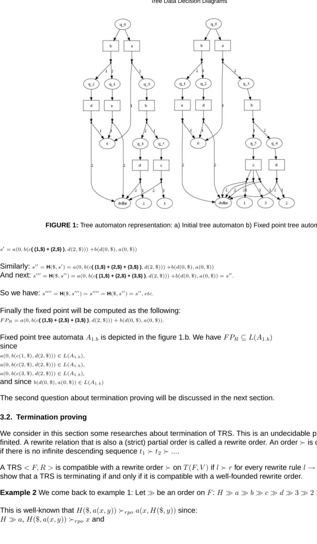
From section 2.2, initial tree automataA1.ais depicted in the figure 1.a. We haves⊆L(A1.a) sincea(0, b(c(1,$), d(2,$)))∈L(A1.a) : q0(a(0, b(c(1,$), d(2,$)))) −→a(¯0(0), q3(b(c(1,$), d(2,$)))) −→a(0, b(q5(c(1,$)), q4(d(2,$)))) −→a(0, b(c(¯1(1),¯$($)), d(¯2(2),¯$($)))) −→a(0, b(c(1,$), d(2,$)))
and sinceb(d(0,$), a(0,$))∈L(A1.a) :
q0(b(d(0,$), a(0,$)))
−→b(q2(d(0,$)), q1(a(0,$)))
−→b(d(¯0(0),¯$($)), a(¯0(0),¯$($))) −→b(d(0,$), a(0,$))
The simplification is as the following:
s0=H($, s)
r4,r7,r8
−−−−−−→
a(0,H($, b(c(1,$), d(2,$))))
+b(H($, d(0,$)), a(0,$)) +b(d(0,$),H($, a(0,$)))
and then we have:
a(0,H($, b(c(1,$)], d(2,$)))) r7,r8 −−−−→a(0, b(H($, c(1,$)), d(2,$))) +a(0, b(c(1,$),H($, d(2,$)))) r6,r5 −−−−→a(0, b(c(H($,1),$), d(2,$))) +a(0, b(c(1,$), d(2,H($,$)))) r2,r0 −−−−→a(0, b(c(2,$), d(2,$))) +a(0, b(c(1,$), d(2,$))) andb(H($, d(0,$)), a(0,$)) +b(d(0,$),H($, a(0,$))) r5,r4 −−−−→b(d(0,H($,$)), a(0,$)) +b(d(0,$), a(0,H($,$))) r0,r0 −−−−→b(d(0,$), a(0,$)) +b(d(0,$), a(0,$))
The factorization (a(0, b(c(2,$), d(2,$)))+a(0, b(c(1,$), d(2,$))))) and the redundancy elimination (b(d(0,$), a(0,$))+b(d(0,$), a(0,$))
FIGURE 1: Tree automaton representation: a) Initial tree automaton b) Fixed point tree automaton s0=a(0, b(c ( (1,$) + (2,$) ), d(2,$))) +b(d(0,$), a(0,$)) Similarly:s00=H($, s0) =a(0, b(c( (1,$) + (2,$) + (3,$) ), d(2,$))) +b(d(0,$), a(0,$)) And next:s000=H($, s00) =a(0, b(c( (1,$) + (2,$) + (3,$) ), d(2,$))) +b(d(0,$), a(0,$)) =s00. So we have:s0000=H($, s000) =s0000=H($, s00) =s00, etc.
Finally the fixed point will be computed as the following:
F PR=a(0, b(c( (1,$) + (2,$) + (3,$) ), d(2,$))) +b(d(0,$), a(0,$)).
Fixed point tree automataA1.bis depicted in the figure 1.b. We haveF PR⊆L(A1.b)
since
a(0, b(c(1,$), d(2,$)))∈L(A1.b), a(0, b(c(2,$), d(2,$)))∈L(A1.b),
a(0, b(c(3,$), d(2,$)))∈L(A1.b), and sinceb(d(0,$), a(0,$))∈L(A1.b)
The second question about termination proving will be discussed in the next section. 3.2. Termination proving
We consider in this section some researches about termination of TRS. This is an undecidable problem even if F, R finited. A rewrite relation that is also a (strict) partial order is called a rewrite order. An orderÂis called well-founded if there is no infinite descending sequencet1Ât2Â....
A TRS< F, R >is compatible with a rewrite orderÂonT(F, V)iflÂrfor every rewrite rulel→rof R. It is easy to show that a TRS is terminating if and only if it is compatible with a well-founded rewrite order.
Example 2 We come back to example 1: LetÀbe an order onF:H ÀaÀbÀcÀdÀ3À2À1À0À$. This is well-known thatH($, a(x, y))Ârpoa(x, H($, y))since:
H($, a(x, y))ÂrpoH($, y)sinceH =H and{$, a(x, y)} Âmul
rpo {$, y},...
So we can say thatr4is compatible withÂrpo.
Similarly, for other rules,Ris compatible withÂrpo, i.e4Ris simply terminating.
It should be noted that the above order is not unique, e.g. another one can be:HÀdÀcÀbÀaÀ0À1À2À 3 À $. Also notice that we sometime can not find any order. In this case, we try to search a mapπf like semantic
labelling technique presented at the end of section 2.1 providing termination on< Flab, Rlab>.
We do not discuss here the fixed point termination because fixed point termination proving is an undecidable problem, even harder than root reduction problem, there often exists a fixed point is not terminating while its root reduction termination is proved, e.g: let F($, x) −→ a(x, x), F∗($) = $ + a($,$) + a(a($,$), a($,$)) +
a(a(a($,$), a($,$)), a(a($,$), a($,$)))... will be infinite. Intuitively, we find that fixed point termination is a special termination problem in infinite system [10].
4. EXPERIMENTAL IMPLEMENTATIONS AND CASE STUDY 4.1. TRS and tree automaton representation
In this section, we focus on the dining philosophers problem for either DDD simulation or TDDD representation. For DDD simulation, a single philosopher has left hand 0l0 and right hand 0r0 with their values are 0 and 1
(Corresponding with or without fork). DDD system is decribed as a sequence of0l0 and0r0, e.g. the DDD encoding of
four philosophers system can be represented by:l(0, r(1,
| {z } 1stphy l(0, r(1, | {z } 2ndphy l(0, r(1, | {z } 3rdphy l(0, r(1, | {z } 4thphy dollar))))))))
It should be noted that at the same moment, two neighbors never take the same fork, i.e.
l(0, r(1, l(0, r(1, l(1,
| {z }
conf lict
r(1, l(0, r(1, dollar)))))))) is not an accepted configuration.
And DDD TRS simulates the homomorphisms of DDD (Synchronization between two philosophers, the left hand of ithand the right hand ofi+ 1th):
Init: H ( dollar, l ( x, y ) ) -> L ( x, y ); L ( z, r ( x, y ) ) -> l ( z, R ( x, y ) ); Synchronize: R ( z, l ( x, y ) ) -> r ( 0, L ( 1, y ) ); R ( z, l ( x, y ) ) -> r ( 0, L ( 0, y ) ); R ( z, l ( x, y ) ) -> r ( 1, L ( 0, y ) ); End of configuration handle:
R ( z, dollar ) -> r ( z, dollar ); L ( z, dollar ) -> l ( z, dollar );
Synchronization between philosophernthand1st(They are neighbors in the round table):
Change and memorize the left hand of first philosopher:
H ( dollar, l ( x, y ) ) -> r ( 0, M ( 0, y ) ); H ( dollar, l ( x, y ) ) -> r ( 1, N ( 1, y ) ); Go down until the last philosopher:
M ( z, l ( x, y ) ) -> l ( x, M ( z, y ) ); M ( z, r ( x, y ) ) -> r ( x, M ( z, y ) ); N ( z, l ( x, y ) ) -> l ( x, N ( z, y ) ); N ( z, r ( x, y ) ) -> r ( x, N ( z, y ) ); Synchronize with the right hand of last philosopher:
M ( 0, r ( x, dollar ) ) -> l ( 0, dollar ); M ( 0, r ( x, dollar ) ) -> l ( 1, dollar ); N ( 1, r ( x, dollar ) ) -> l ( 0, dollar );
This TRS is not proved terminating on account of the cycle below (i.e we can not determine whether L À R or
RÀL):
L ( z, r ( x, y ) ) -> l ( z, R ( x, y ) ); R ( z, l ( x, y ) ) -> r ( 0, L ( 1, y ) ); R ( z, l ( x, y ) ) -> r ( 0, L ( 0, y ) ); R ( z, l ( x, y ) ) -> r ( 1, L ( 0, y ) );
But we can use semantic labelling with labels are order of philosophers in the system, e.g.:
Li ( z, r ( x, y ) ) -> l ( z, Ri ( x, y ) ); Ri ( z, l ( x, y ) ) -> r ( 0, L(i+1) ( 1, y ) ); Ri ( z, l ( x, y ) ) -> r ( 0, L(i+1) ( 0, y ) ); Ri ( z, l ( x, y ) ) -> r ( 1, L(i+1) ( 0, y ) );
withi= 1, ..., nandÀbe an order onF:H ÀL1ÀR1ÀL2ÀR2À...ÀLnÀRnÀM ÀN À1À0À$.
This TRS is terminating owing to the compatibility with RPO. When a model is proved terminating (called well-designed), the model-checker will generate all of reachability states if the system resources are enough.
We have also built a TDDD representation for dining philosophers problem. Hierarchical model contains:
• 0s0 is a philosophers group (having a different number of philosophers,0s0 higher for group more philosophers) • 0p0 is a philosopher having left hand and right hand with their values 0 and 1 (Corresponding with or without
fork).
For example, a system of four philosophers is like follow (The first0s0 presents the group having four philosophers
while two others in its sub-terms decribe the group of two philosophers):
s(s(p(1,0), | {z } 1stphy p(1,0) | {z } 2ndphy ), s(p(1,0), | {z } 3rdphy p(1,0) | {z } 4thphy )))
TDDD rewriting rule set 1:
Synchronization between two philosophersithandi+ 1th:
H ( dollar, s ( x, y ) ) -> A ( x, y ); A ( s ( x, y ), s ( u, v ) ) -> s ( A ( x, y ), s ( u, v ) ); A ( s ( x, y ), s ( u, v ) ) -> s ( s ( x, y ), A ( u, v ) ); A ( p ( x, y ), p ( u, v ) ) -> s ( p ( x, 0 ), p ( 0, v ) ); A ( p ( x, y ), p ( u, v ) ) -> s ( p ( x, 1 ), p ( 0, v ) ); A ( p ( x, y ), p ( u, v ) ) -> s ( p ( x, 0 ), p ( 1, v ) ); H ( dollar, s ( x, y ) ) -> B ( x, y ); B ( s ( w, s ( u, v ) ), s ( s ( x, y ), z ) ) -> s ( B ( w, s ( u, v ) ), s ( s ( x, y ), z ) ); B ( s ( w, s ( u, v ) ), s ( s ( x, y ), z ) ) -> s ( s ( w, s ( u, v ) ), B ( s ( x, y ), z ) ); B ( s ( w, s ( u, v ) ), s ( s ( x, y ), z ) ) -> s ( D ( w, s ( u, v ) ), G ( s ( x, y ), z ) ); B ( s ( w, s ( u, v ) ), s ( s ( x, y ), z ) ) -> s ( R ( w, s ( u, v ) ), L ( s ( x, y ), z ) ); B ( s ( w, p ( u, v ) ), s ( p ( x, y ), z ) ) -> s ( s ( w, p ( u, 0 ) ), s ( p ( 0, y ), z ) ); B ( s ( w, p ( u, v ) ), s ( p ( x, y ), z ) ) -> s ( s ( w, p ( u, 1 ) ), s ( p ( 0, y ), z ) ); B ( s ( w, p ( u, v ) ), s ( p ( x, y ), z ) ) -> s ( s ( w, p ( u, 0 ) ), s ( p ( 1, y ), z ) ); G ( s ( u, v ), s ( x, y ) ) -> s ( G ( u, v ), s ( x, y ) ); G ( p ( u, v ), p ( x, y ) ) -> s ( p ( 0, v ), p ( x, y ) ); D ( s ( u, v ), s ( x, y ) ) -> s ( s ( u, v ), D ( x, y ) ); D ( p ( u, v ), p ( x, y ) ) -> s ( p ( u, v ), p ( x, 1 ) ); D ( p ( u, v ), p ( x, y ) ) -> s ( p ( u, v ), p ( x, 0 ) ); R ( s ( u, v ), s ( x, y ) ) -> s ( s ( u, v ), R ( x, y ) ); R ( p ( u, v ), p ( x, y ) ) -> s ( p ( u, v ), p ( x, 0 ) ); L ( s ( u, v ), s ( x, y ) ) -> s ( L ( u, v ), s ( x, y ) ); L ( p ( u, v ), p ( x, y ) ) -> s ( L ( 0, v ), p ( x, y ) ); L ( p ( u, v ), p ( x, y ) ) -> s ( L ( 1, v ), p ( x, y ) );
Synchronization between philosophernthand1st:
H ( dollar, s ( x, y ) ) -> C ( x, y ); C ( s ( u, v ), s ( x, y ) ) -> s ( U ( u, v ), V ( x, y ) ); C ( s ( u, v ), s ( x, y ) ) -> s ( M ( u, v ), N ( x, y ) ); U ( s ( u, v ), s ( x, y ) ) -> s ( U ( u, v ), s ( x, y ) ); U ( p ( u, v ), p ( x, y ) ) -> s ( p ( 0, v ), p ( x, y ) );
V ( s ( u, v ), s ( x, y ) ) -> s ( s ( u, v ), V ( x, y ) ); V ( p ( u, v ), p ( x, y ) ) -> s ( p ( u, v ), p ( x, 0 ) ); V ( p ( u, v ), p ( x, y ) ) -> s ( p ( u, v ), p ( x, 1 ) ); M ( s ( u, v ), s ( x, y ) ) -> s ( M ( u, v ), s ( x, y ) ); M ( p ( u, v ), p ( x, y ) ) -> s ( p ( 0, v ), p ( x, y ) ); M ( p ( u, v ), p ( x, y ) ) -> s ( p ( 1, v ), p ( x, y ) ); N ( s ( u, v ), s ( x, y ) ) -> s ( s ( u, v ), N ( x, y ) ); N ( p ( u, v ), p ( x, y ) ) -> s ( p ( u, v ), p ( x, 0 ) ); LetÀbe an order onF:H ÀAÀCÀDÀGÀRÀLÀM ÀN ÀU ÀV ÀsÀpÀ1À0À$.
This TRS is terminating because of the compatibility with RPO. As we previously mentioned, this model is well-designed, the model-checker will generate all of reachability states if the system resources are enough.
Tree automaton representation of fixpointF PR with 18 states for 81 reachability configurations (In other words, term
setF PRcontains 81 different terms where each term corresponds to a system configuration) is shown in the figure
2. We can recognize the compact data from the sharing states.
FIGURE 2: Fixpoint of Dining Philosophers with n = 4
4.2. Result analysis
We aim at comparing DDD and TDDD in the same data structure and test them in the same environment. The code is written in JAVA and ran in a normal PC 1.7GHz, 1G RAM.
First, we prove successfully the termination of models for DDD and TDDD, i.e. the model-checker either for DDD or TDDD will return all of reachability states if the system resources are enough.
The result in the table shows that TDDD has a better sharing internal data structure than DDD owing to the hierarchical architecture. So DDD has a smaller time complexity but it fails rapidly when the size of test models increases exponentially.
DDD DDD TDDD TDDD
n #Configurations Time(s) States Time (s) States
4 34 4 23 8 18
8 38 - - 59 26
16 316 - - 407 34 32 332 - - 2718 45
The TRS system design is very important. Because of the redundant rules elimination and our others experiences in implementation, we can reduce to an equivalent rewriting rule set 2 with#R= 19andV ={x, y}(Instead of rewriting rule set 1 with#R= 37andV ={x, y, u, v}):
Synchronization between two philosophersithandi+ 1th:
H ( dollar, x ) -> A ( dollar, x ); A ( dollar, s ( x, y ) ) -> s ( G ( dollar, x ), D ( dollar, y ) ); A ( dollar, s ( x, y ) ) -> s ( L ( dollar, x ), R ( dollar, y ) );
Synchronization between two philosophersnthand1st:
H ( dollar, x ) -> B ( dollar, x ); B ( dollar, s ( x, y ) ) -> s ( B ( dollar, x ), y ); B ( dollar, s ( x, y ) ) -> s ( x, B ( dollar, y ) ); B ( dollar, s ( x, y ) ) -> s ( R ( dollar, x ), L ( dollar, y ) ); B ( dollar, s ( x, y ) ) -> s ( D ( dollar, x ), G ( dollar, y ) );
And the sharing primitive rule:
L ( dollar, s ( x, y ) ) -> s ( L ( dollar, x ), y ); R ( dollar, s ( x, y ) ) -> s ( x, R ( dollar, y ) ); L ( dollar, p ( x, y ) ) -> p ( V ( dollar, x ), y ); R ( dollar, p ( x, y ) ) -> p ( x, U ( dollar, y ) ); G ( dollar, s ( x, y ) ) -> s ( G ( dollar, x ), y ); D ( dollar, s ( x, y ) ) -> s ( x, D ( dollar, y ) ); G ( dollar, p ( x, y ) ) -> p ( U ( dollar, x ), y ); D ( dollar, p ( x, y ) ) -> p ( x, V ( dollar, y ) ); U ( dollar, x ) -> 1 ; U ( dollar, x ) -> 0 ; V ( dollar, x ) -> 0 ; LetÀbe an order onF:H ÀAÀB ÀLÀRÀGÀDÀU ÀV À1À0À$. This TRS is terminating on account of the compatibility with RPO.
Automata TDDD with RuleSet 1 TDDD with RuleSet 2
n States Time(s) Time (s)
4 18 8 0 8 26 59 3 16 34 407 23 32 45 2718 311 64 60 59724 3505 128 121 - 62395
Obviously, the reduction of rule set and variable set (RuleSet 2) brings the better time complexity than RuleSet 1, we call it informally the better-designed among well-designed models. It should be noted that tree automaton is the same for both RuleSet 1 or RuleSet 2, that can be explained by the fact that the better-designed improves only the time complexity but it can not change the space complexity.
In fact, a model-checker of distributed systems verification [7] based on a formal language LfV (Language for Verification) [6] using DDD in MORSE [5], an industry and academic cooperation RNTL project can compute the local fixpoints generating the result more rapid.
Actually, the global fixpoint in TRS increases the time complexity of TDDD, each step we must start the fixpoint computation from root of the automaton and move downward by storing a large temporary results. The integration of
local fixpoints technique (like in DDD and SDD) into TDDD will progress the time complexity of this model-checker in this case.
5. CONCLUSION
We proposed a new extension of DDD for symbolic verification in TRS. It is not only compact as SDD (more than DDD) but its operators are also very simpler and more flexibly than the others on account of TRS interface.
Moreover, we prove successfully the termination of models for DDD and TDDD in some particular cases and support model design orientation for developers. On the other hand, presenting terms by tree automata technique provides the capability to maintain the internal representation of data in canonical form though the time complexity of the factorization is still a challenge.
For future works, first, we aim at integrating into TDDD the local fixpoints technique which is implemented successfully in DDD and SDD to improve the time complexity of TDDD checker. Finally, we plan to develop a TDDD model-checker for the infinite TRS< F, R >. In this case, we must use minimization algorithm for non-deterministic tree automaton like bisimulation minimization [14, 15].
REFERENCES
[1] Bryant, R.E. (1986) Graph-Based Algorithms for Boolean Function Manipulation. IEEE Transactions on Computers volume 35,number 8, pages 677-691.
[2] Couvreur, J-M. and Encrenaz,E. and PaviotAdet,E. and Poitrenaud, D. and Wacrenier, P. (2002) Data Decision
Diagram for Petri Net Analysis. ICATPN, volume 2360, pages 101-120, Springer Verlag.
[3] Couvreur, J-M. (2004) Contribution `a l’algorithme de la v ´erification. M ´emoire d’habilitation `a diriger des recherches, LaBRI,Universit ´e Bordeaux 1, France.
[4] Couvreur,J-M. and Thierry-Mieg,Y. (2005) Hierarchical Decision Diagrams to Exploit Model Structure. FORTE, pages 443-457, http://dx.doi.org/10.1007/11562436 32.
[5] Kordon,F. and Lemoine, M. (2004) Formal methods for embedded distributed systems: how to master the
complexity. ISBN 1-4020-7996-6, Kluwer Academic Publishers, Norwell, MA, USA.
[6] Nguyen,D-T. (2006) LfV, Language for Verification.7thSchool on MOdelling and VErifying of parallel Processes,
pages 336-341, Bordeaux, France.
[7] Nguyen,D-T. (2007) LfV-DDD Checker.5thIEEE International Conference on Research, Innovation and Vision
for the Future, pages 165-166, Hanoi, Vietnam
[8] Ohlebusch,E. (2002) Advanced topics in term rewriting. ISBN 0-387-95250-0, Springer-Verlag, London, UK. [9] Zantema,H. (2003) Term rewriting system, chapter Termination, ISBN 0-521-39115-6, Cambridge University
Press, UK.
[10] Ohlebusch,E. (1992) A Note on Simple Termination of Infinite Term Rewriting Systems. report nr. 7, Universitat Bielefeld, url ”citeseer.ist.psu.edu/ohlebusch92note.html”.
[11] Zantema, H. (2005) Termination of string rewriting proved automatically. Journal of Automated Reasoning, volume 34, pages 105-139, Springer Verlag, London, UK.
[12] Zantema, H. (1995) Termination of Term Rewriting by Semantic Labelling. Journal Fundamenta Informaticae, volume 24, number 1/2, pages 89-105, url ”citeseer.ist.psu.edu/zantema95termination.html”.
[13] H. Comon and M. Dauchet and R. Gilleron and C. L ¨oding and F. Jacquemard and D. Lugiez and S. Tison and M. Tommasi (2007) Tree Automata Techniques and Applications. Available on: url ”http://www.grappa.univ-lille3.fr/tata”, release October, 12th 2007.
[14] Abdulla P. A., Hogberg J. and Kaati L. (2006) Bisimulation Minimization of Tree Automata. CIAA, pages 173-185, url ”http://dx.doi.org/10.1007/11812128 17”, Springer-Verlag, London, UK.
[15] Paige R. and Tarjan R. E. (1987) Three partition refinement algorithms. Journal SIAM J. Comput., volume 16, number 6, issn 0097-5397, pages 973-989, url ”http://dx.doi.org/10.1137/0216062”, Society for Industrial and Applied Mathematics, Philadelphia, PA, USA.