Technological University Dublin Technological University Dublin
ARROW@TU Dublin
ARROW@TU Dublin
Session 2: Deep Learning for Computer Vision IMVIP 2019: Irish Machine Vision and Image Processing 2019Comparing Data Augmentation Strategies for Deep Image
Comparing Data Augmentation Strategies for Deep Image
Classification
Classification
Sarah O'GaraDublin City University
Kevin McGuinness
Dublin City University
Follow this and additional works at: https://arrow.tudublin.ie/impstwo
Part of the Electrical and Computer Engineering Commons Recommended Citation
Recommended Citation
O'Gara, S. & McGuinness, K. (2019). Comparing data augmentation strategies for deep image
classification. IMVIP 2019: Irish Machine Vision & Image Processing, Technological University Dublin, Dublin, Ireland, August 28-30. doi:10.21427/148b-ar75
This Article is brought to you for free and open access by the IMVIP 2019: Irish Machine Vision and Image
Processing at ARROW@TU Dublin. It has been accepted for inclusion in Session 2: Deep Learning for Computer Vision by an authorized administrator of ARROW@TU Dublin. For more information, please contact
[email protected], [email protected], [email protected].
This work is licensed under a Creative Commons Attribution-Noncommercial-Share Alike 3.0 License
Comparing Data Augmentation Strategies for Deep Image
Classification
Sarah O’Gara and Kevin McGuinness
School of Electronic Engineering, Dublin City University
Abstract
Currently deep learning requires large volumes of training data to fit accurate models. In practice, however, there is often insufficient training data available and augmentation is used to expand the dataset. Historically, only simple forms of augmentation, such as cropping and horizontal flips, were used. More complex augmentation methods have recently been developed, but it is still unclear which techniques are most effective, and at what stage of the learning process they should be introduced. This paper investigates data augmentation strategies for image classification, including the effectiveness of different forms of augmentation, dependency on the number of training examples, and when augmentation should be introduced during training. The most accurate results in all experiments are achieved using random erasing due to its ability to simulate occlusion. As expected, reducing the number of training examples significantly increases the importance of augmentation, but surprisingly the improvements in generalization from augmentation do not appear to be only as a result of augmentation preventing overfitting. Results also indicate a learning curriculum that injects augmentation after the initial learning phase has passed is more effective than the standard practice of using augmentation throughout, and that injection too late also reduces accuracy. We find that careful augmentation can improve accuracy by +2.83% to95.85%using a ResNet model on CIFAR-10 with more dramatic improvements seen when there are fewer training examples. Source code is available at
https://git.io/fjPPy
Keywords:data augmentation, image classification, supervised learning, CNN, CIFAR-10
1
Introduction
Current supervised learning techniques require large volumes of training data to train accurate models. Deep models have become more complex and with this complexity has emerged new challenges. These challenges include gradient vanishing, overfitting, hardware limitations, and hyper-parameter optimization. One of the most important challenges that continuously hinders the application of deep learning is insufficient training data. A lack of data often leads to overfitting due to the limited supply of examples that the network can learn from. Many techniques have been proposed to limit overfitting, including dropout, transfer learning, and data augmentation [Srivastava et al., 2014, Huang et al., 2017, Perez and Wang, 2017]. Data augmentation techniques seek to expand the amount of training data automatically by applying automatic transformations to images. Traditional augmentation techniques include horizontal image flips, cropping, translations, and rotation. Recently, more complex augmentation techniques such as elastic distortion, tilting, and theme adjustments have been developed. The effectiveness of the newly developed techniques in preventing overfitting, improving accuracy, and the effect on training times has not yet been fully explored. It is also still unclear when in the training process data augmentation should be introduced.
This paper investigates several augmentation strategies using a state-of-the-art ResNet model trained with stochastic gradient descent (SGD) on CIFAR-10. Subsets of CIFAR-10 with 200 and 1,000 samples per class are used to explore the effect of sample size on performance. We compare the different augmentation strategies using six different forms of augmentation: rotation, skew, shear, random erasing, random distortion, and Gaussian distortion.
2
Related Work
An area that benefits greatly from data augmentation is the medical industry, where there is little data available to train networks. [Hussain et al., 2018] looked at the effects of data augmentation for the binary classification problem of mass identification, exploring to what extent the augmented data retains properties of the original medical imagery. The original dataset consisted of 1,650 mass case images and 1,651 non-mass cases, from the Digital Database for Screening Mammography [Heath et al., 2000]. The augmentation techniques tested were flips, Gaussian noise, jittering, scaling, powers, Gaussian blur, rotations, and shearing. Each augmentation was tested using a separate pre-trained VGG-16 network [Simonyan and Zisserman, 2015]. The paper notes that particular attention is needed when choosing the hyper-parameters of the augmentation techniques, to ensure class preservation. Overall, the results indicate that noise is the least effective augmentation technique with a validation accuracy of 66%. The most effective augmentation techniques were the Gaussian filter at 88.1% and rotation at 88%. All other techniques performed reasonably well with accuracy ranges of 81.3% to 87.9%. The networks visualization of a mass object varies significantly depending on the type of augmentation used, indicating that augmentation has an effect on the networks learning patterns.
[Shijie et al., 2017] investigated the effects of data augmentation on a multi classification problem using AlexNet as the pre-trained model. A subset of 10 classes was selected from ImageNet with 6,000 images randomly selected from each category. The training set was grouped into three different scales: small (200-samples per class), medium (1000-(200-samples per class), and large (5000-(200-samples per class). The augmentation techniques used can be divided into unsupervised and supervised augmentation techniques, which included generative adversarial networks (GAN) and its improved versions such as WGAN [Goodfellow et al., 2014]. Augmentation techniques were tested individually, with the most successful combined for further testing. The dataset was doubled and tripled in size using the different augmentation techniques, with smaller datasets showing significantly better percentage increases in accuracy. The paper suggests that triple combinations can degrade performance. This is possibly due to the images being augmented too severely by triple combinations for class preservation.
[Zhong et al., 2017] purposed random erasing as a means to make models more robust to occlusion. Usually training examples exhibit little variation in occlusion. This means models can be susceptible to overfitting and tend to generalize poorly to unseen data that may not exhibit all features of the class. Random erasing randomly removes information from a region of the image, reducing reliance on particular features being present and thus improving generalization. This is analogous to the reduction of co-adaption in the network through the use of dropout. A baseline was established for the CIFAR-10, CIFAR-100, and Fashion MNIST datasets for ResNet models of various depths. The models were then trained using random erasing, combined with the standard augmentation techniques used on the original dataset. All models were shown to give an improvement in accuracy with the ResNet-56 model having an error of just 4.89% compared to 5.31%.
3
Method
3.1 Model and Optimizer
We use an adaptation of the popular ResNet model in all experiments. ResNet achieved a Top-5 error rate of 3.57% in ImageNet ILSVRC (using an ensemble) by addressing the issues of gradient vanishing/exploding [He et al., 2015]. Previous work by [Simonyan and Zisserman, 2015] had shown that the accuracy of the net-works is improved by depth. A problem with increasing depth is the accuracy saturates and degrades rapidly, but the cause is not overfitting. ResNet mitigates these issues by introducing deep residual learning blocks to the network. The input to the ReLU is given asF(x)+x, i.e. shortcut connections are introduced to the network. This allows the depth of the network to be increased to 152-layers while maintaining a lower computational com-plexity than VGG-16 with no degradation. [He et al., 2015] presents an adaption of the model (ResNet-56) for use with32×32images that obtained an error rate of 6.97% on CIFAR-10, which we adopt in our experiments. We use SGD with Nestrov momentum as the optimizer for all experiments, which is one of the most
commonly used optimizers for convolutional neural networks in classification tasks. Momentum is impor-tant to accelerate SGD and dampen the gradient oscillations in regions where the curvature of the loss sur-face varies widely in different directions. Although there are more sophisticated first order optimizers (e.g. Adam [Kingma and Ba, 2015]) that consistently improve the loss faster in the initial epochs, SGD has been observed to reach a local minima with lower overall loss and better generalization properties [Ruder, 2016]. 3.2 Datasets
The selection of the dataset is extremely important to deep learning models. More examples from each class with higher variation reduces the risk of a bias and overfitting. For classification tasks, models should be provided with an equal number of examples from each class, reducing the risk of class bias. For this reason, we opt to test the different augmentation strategies using CIFAR-10.
CIFAR-10 consists of32×32colour images from 10 mutually exclusive classes: airplane, automobile, bird, cat, deer, dog, frog, horse, ship and truck [Krizhevsky, 2009]. There are 50,000 training and 10,000 test images with an equal number of images selected from each class. Due to the small image resolution, careful consideration is needed when selecting data augmentation techniques.
We randomly sample the dataset to create a 200 samples per class and 1,000 samples per class dataset, reducing the training examples available to 4% and 20% of the original dataset. The effects of overfitting and model generalization as noted in [Hussain et al., 2018, Shijie et al., 2017] are more pronounced with data scarcity. Therefore, we experiment at three specified sample sizes: 5,000 samples per class (large), 1,000 samples per class (medium), and 200 samples per class (small).
3.3 Augmentations
Augmentation is implemented in the training process using the Augmentor library [Bloice et al., 2017]. Augmen-tation is completed on-the-fly for each batch. Online augmenAugmen-tation benefits from the generation of more unique training images than offline augmentation but produces longer training times [Andersson and Berglund, 2018]. Any artefacts produced by augmentation are removed by automatic image cropping and resizing. We investigate the following forms of augmentation:
Rotation: A random rotation of maximum ±25◦ ensures severe cropping does not remove defining class
features. Due to the nature of the classes, rotation outside this range would create unrealistic examples. Skew Tilt: The image is tilted forwards, backwards, left, or right a maximum of 22.5°. This gives the illusion that the image is being viewed from a different perspective than originally seen and creates realistic examples. Shear: Stretches the image in one of the axial planes, i.e. shear occurs along the x-axis or y-axis. A maximum shear of±20◦is used to ensure class preservation.
Random Erase: The pixels within a random rectangular area are set to random RGB values. The maximum area effected by the augmentation is 50% of the pixels.
Random Distortion: The parameters of this distortion are given in terms of grid width, grid height, and magnitude. The granularity of the distortion is controlled by the grid width and height, representing the number of horizontal and vertical divisions to apply distortion to. Both values are chosen as 6, and the magnitude of the distortion is chosen as 5. As images are only32×32pixels, distortion is expected to produce unrealistic examples.
Gaussian Distortion: Grid width and height, and magnitude are kept the same as the random distortion values of 6, 6, and 5, respectively. The Gaussian distortion has the added parameters of applying the distortion based on the 2D normal distribution:
p(x,y)=exp ( − Ã (x−µx)2 σx + (y−µy)2 σy !) . (1)
The normal distortion is applied to each grid point on a circular surface (corner="bell") and with default values for the mean and standard deviation (µx=µy=0.5,σx=σy=0.05).
3.4 Experiments
First we establish a baseline for the ResNet-56 model on the CIFAR-10 dataset trained for 163 epochs. The training set is transformed by random crops to 32x32 images with a padding of 4, random horizontal flips, conversion to a tensor, and normalized with mean [0.4914, 0.4822, 0.4465] and standard deviation [0.2023, 0.1994, 0.2010]. The validation set is transformed by a conversion to a tensor, and the same normalization. Images are loaded in batches of 128. We use an initial learning rate of 0.1, momentum of 0.9, and weight decay of10−4for the optimizer. The learning rate is divided by 10 on epochs 81 and 122, similar to [He et al., 2015]. All parameters are kept constant throughout experiments unless stated otherwise. Augmentations are tested individually by doubling the dataset, and compared to the baseline results.
[Hussain et al., 2018] used a pre-trained model to test augmentation strategies. This fine-tuning of the model using the desired dataset is known as transfer learning. For effective fine-tuning, the new dataset must be similar to the dataset used to train the model. Augmentation can be seen as a method of fine-tuning the baseline model. We introduce augmentation on epochs 30, 60, and 90 of the baseline model and continue training until epoch 163 to discover the optimal time to introduce augmentation. Epochs 30, 60, and 90 represent three distinct stages in the training process: initial loss rate stabilising, loss rate stagnate before learning rate decrease, and loss rate stagnate after learning rate decrease.
We use the small and medium datasets to train the model similar to [Shijie et al., 2017]. The learning rate and batch size are related to the generalization performance of models as shown by [Masters and Luschi, 2018]. The range of learning rates that provide a stable convergence reduces as batch size increases. In the most extreme case, we reduce the training set to 4% of the original dataset, meaning a batch size of 128 would likely degrade performance. [Keskar et al., 2016] also shows degrading performance for large batches. Large batches tend to converge to sharp minimizers leading to poor generalization due to the numerous large eigenvalues in the Hessian on convergence. Small batches, on the other hand, tend to converge to flat minimizers, which have smaller Hessian eigenvalues. They generate more noise in gradient calculations, decreasing the chance of the gradient dropping into a sharp local minima. Based on these observations, we train the small and medium datasets using three learning rate strategies: 1) the original strategy from [He et al., 2015], 2) using a batch size of 128 with no learning rate schedule, and 3) using a batch size of 8 with original learning rate schedule.
4
Results & Discussion
4.1 Single Augmentations
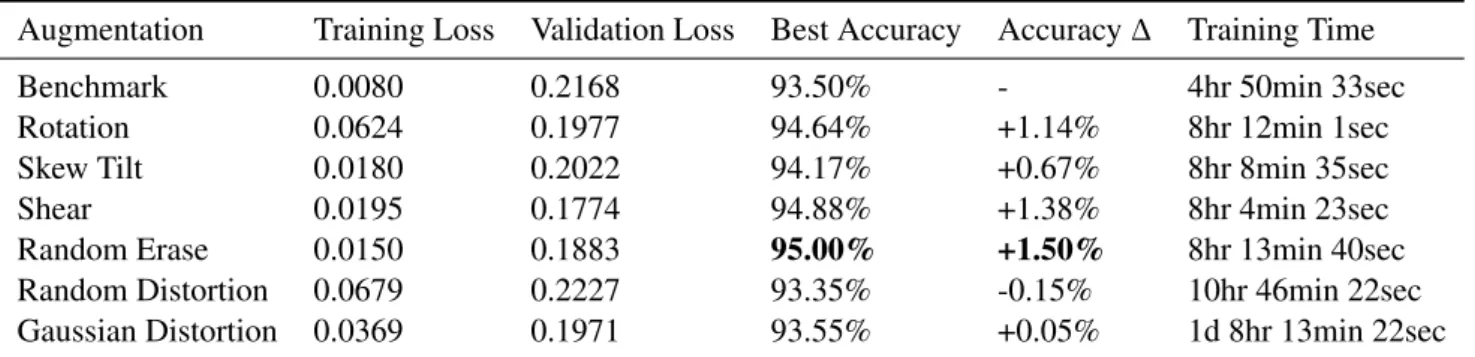
Table 1 shows the single augmentation and benchmark results when trained using a single NVIDIA GTX 1080 Ti. The benchmark obtains the lowest training loss, although this gives no indication of the model’s performance on unseen data. When we compare the validation and training loss, the margin between the two indicates the benchmark model is overfitting. Augmentation models exhibit smaller margins, indicating augmentation reduces overfitting in CIFAR-10.
Random erasing shows the best improvement in accuracy of+1.5%. Both distortion augmentations obtain worse or similar results to the baseline. Due to the nature of the classes, the augmented images produced are often unrealistic, confirming that the augmentation must be relevant to the task: the model is trained to be robust to distortions that never occur in practice.
Augmentation Training Loss Validation Loss Best Accuracy Accuracy∆ Training Time
Benchmark 0.0080 0.2168 93.50% - 4hr 50min 33sec
Rotation 0.0624 0.1977 94.64% +1.14% 8hr 12min 1sec
Skew Tilt 0.0180 0.2022 94.17% +0.67% 8hr 8min 35sec
Shear 0.0195 0.1774 94.88% +1.38% 8hr 4min 23sec
Random Erase 0.0150 0.1883 95.00% +1.50% 8hr 13min 40sec
Random Distortion 0.0679 0.2227 93.35% -0.15% 10hr 46min 22sec
Gaussian Distortion 0.0369 0.1971 93.55% +0.05% 1d 8hr 13min 22sec
Table 1: Results for single augmentations. Best accuracy shown for random erasing.
The complexity of the augmentation effects the overall training time. Traditional, more simplistic augmenta-tions require little processing time, leading to increases in training time of∼3.5hours. Gaussian distortion sees the most significant increase in training time of 665%. We discovered this is due to the computational expense of generating the augmented images.
Figure 1: Learning curve for Multi-Single Augmentation training. Dataset split into groups of 50k images augmented using random erasing, rotation, shear, and skew.
Figure 1 shows the learning curve for the dataset expanded using random erasing, rotation, shear, and skew tilt. We apply each augmentation separately, leading to the dataset increasing from 50k training images to 250k. This leads to the most accurate result seen throughout all experiments of 95.85%. This strategy only requires an additional 2 hours to train over a single augmentation at 10 hours, 39 minutes, and 51 seconds. At this level of accuracy it is extremely difficult to make further improvements. This result indicates augmentation is a means of making these improvements but at the cost of longer training times. Our method of
applying several single augmentations produces better generalization properties. It improves the robustness of the features learned due to the increase in variance of the training data.
4.2 Varying Augmentation Injection Epoch
Augmentation Injection Epoch: Best Accuracy
1 30 60 90 Benchmark 93.50% - - -Rotation 94.64% 94.76% 94.39% 93.71% Skew Tilt 94.17% 94.93% 94.40% 94.07% Shear 94.88% 94.91% 94.31% 94.13% Random Erase 95.00% 95.05% 94.56% 94.30% Random Distortion 93.35% 93.66% 93.47% 93.07% Gaussian Distortion 93.55% 94.31% 93.94% 93.69% Table 2: Accuracy for introduction of augmentation to training process at varying epochs.
Table 2 indicates that epoch 30 is the opti-mal time to introduce augmentation. By in-jecting augmentation on the30t hepoch, the model combats the effects of overfitting bet-ter with increases in accuracy from +0.05% up to +0.76%. Epoch 30 is the point in the training process when the reduction in loss rate begins to decrease drastically, i.e. the model falls into a local minima point. We conclude that augmentation should be in-troduced into the training process once the initial training phase has passed to improve generalization. The slight improvements in accuracy over the baseline result for
intro-duction at epoch 90 support this conclusion. The model has already overfit the training data and can no longer benefit from the augmentation’s generalization properties. Epoch 60 presents a more interesting point in the training process. The form of augmentation appears to dictate whether the model will have better generalization properties than training with augmentation from scratch but will always be worse than injection at epoch 30.
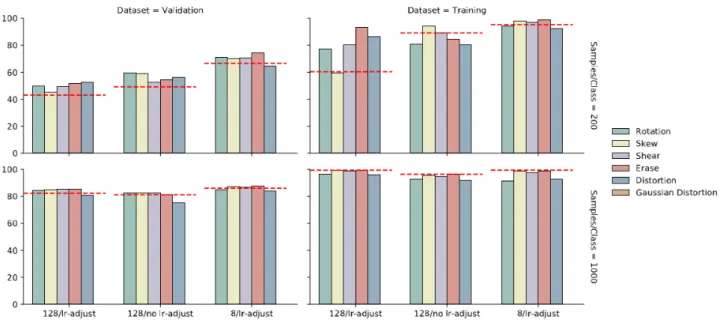
Figure 2: Best accuracy achieved for 200 samples per class (top) and 1,000 samples per class (bottom) on validation (right) and training (left) datasets, with various batch sizes and learning rate schedules. Red dashed lines represent baseline accuracies achieved for each scenario.
4.3 Varying Sample Size
Figure 2 shows the best accuracy achieved over 163 epochs for each model on the small and medium datasets. We test each model using three different combinations of batch size and learning rate schedule based on the observations of [Masters and Luschi, 2018, Keskar et al., 2016], whereby the correlation between the learning rate and batch size can cause a failure to converge.
For the small dataset, by decreasing the batch size from 128 to 8, the validation accuracy is shown to improve by+31.45%using random erasing (74.46%) when compared to the baseline (43.01%). This result indicates that augmentation is most effective in training when data is scarce. We note that overfitting, as measured by high accuracy on the training set, in many of the augmentation results is more severe than for the baseline. This would contradict current assumptions that augmentation improves generalization by preventing overfitting in the case of all NNs [Krizhevsky et al., 2017]. In many of these cases where augmentation has proven to prevent overfitting the sample size for each class is large. In this case the sample size is very small, and overfitting is actually more significant. However, the generalization of the model is better in the presence of augmentation. We hypothesise that, for small datasets, augmentation does not prevent overfitting but, due to the increase in training data, still provides better generalization. With smaller datasets using augmentation increases the models ability to learn certain features present in the training set as augmentation can only alter the data already available, i.e. the model will see similar images twice as much so is more likely to overfit. However, as there is some variance present in the images, the generalization properties of the model still improve.
For the medium dataset, the best accuracy is achieved by random erasing trained with a batch size of 8 at 87.45%, which is an improvement of+6.3%over the baseline. The importance of the learning rate adjustment schedule is apparent with the accuracy decreasing for each model when not applied. However, the improvements in accuracy due to batch size are less significant as suggested by [Masters and Luschi, 2018]. Augmentation does reduce overfitting with the most significant decrease occurring for the small batch size. The generalization of the model also improves. At this scale, augmentation has similar effects on accuracy as seen in the full dataset. When the model has large volumes of training data available, augmentation only slightly increases the generalization capabilities of the network as a large amount of variance already exists. We believe, from these results, that augmentation serves a different purpose at different sample sizes. With data scarcity augmentation acts as a means to increase generalization by increasing the variance in the training set, and in large datasets augmentation acts as a regularizer to prevent overfitting with only slight improvements in generalization.
5
Conclusion
Augmentation leads to a significant increase in training time, likely due to augmentation making it harder for the model to learn. The initial augmentation gives rise to the most significant increase in training time with any additional augmentations adding little overhead. However, a key factor in this increase in training time is the processing time required to apply said augmentation to the dataset, which must be considered when choosing a form of augmentation to apply.
We found combining multiple single augmentations with the original dataset is the most effective augmenta-tion strategy with an increase in accuracy of +2.36% to95.85%. Random distortion and Gaussian distortion are the worst forms of augmentation tested leading to changes in accuracy of -0.15% and +0.05%, respectively. This is due to the augmented images not representing the original class and highlights the importance of the choice of augmentation. The most effective form of single augmentation is found to be random erasing with an increase in accuracy of +1.5%. This is due to its ability to combat the effects of occlusion, and is similar to preventing co-adaption through the use of dropout.
An interesting avenue to explore is the generalization and overfitting properties of augmentation for data scarcity. Validation accuracy is seen to improve with augmentation, with the most significant improvement of +31.45%for random erasing, indicating better generalization capabilities. However, the model also appears to overfit the training data more. This phenomenon does not occur for large datasets and the cause for this at smaller sample sizes should be further explored.
Exploring the interaction of augmentation with more advanced optimizers such as the Adam optimizer, could lead to further improvements in accuracy and training times. Previous work by [Keskar and Socher, 2017], has shown that the generalization gap between SGD and Adam can be reduced by switching from Adam to SGD during the training process. During the switching process the learning rate for SGD is calculated as noted in [Keskar and Socher, 2017] and must be switched at the optimal time to ensure better generalization properties. Building on this approach, the optimizer switching approach could be combined with data augmentation potentially yielding improvements in accuracy.
Injecting augmentation at epoch 30 yielded the best improvements in accuracy for single augmentations, indi-cating a learning curriculum is most effective for augmentation. Late injection of augmentation improves the gen-eralization capabilities of the network similar to the optimizer switching method of [Keskar and Socher, 2017]. As multiple single augmentations could produce a more accurate model (95.85%) than the single augmentations (95.00%), introducing this augmentation strategy at epoch 30 of the training process could potentially improve results further. This would confirm that the generalization properties of the network are optimized by introducing augmentation after the initial learning phase has passed.
Acknowledgments
This publication has emanated from research conducted with the financial support of Science Foundation Ireland (SFI) under grant number SFI/15/SIRG/3283 and SFI/12/RC/2289.
References
[Andersson and Berglund, 2018] Andersson, E. and Berglund, R. (2018). Evaluation of data augmentation of MR images for deep learning. Technical report, Lund University.
[Bloice et al., 2017] Bloice, M. D., Stocker, C., and Holzinger, A. (2017). Augmentor: An image augmentation library for machine learning. CoRR, abs/1708.04680.
[Goodfellow et al., 2014] Goodfellow, I. J., Pouget-Abadie, J., Mirza, M., Xu, B., Warde-Farley, D., Ozair, S., Courville, A., and Bengio, Y. (2014). Generative adversarial nets. InProceedings of the 27th International
Conference on Neural Information Processing Systems - Volume 2, NIPS’14, pages 2672–2680, Cambridge, MA, USA. MIT Press.
[He et al., 2015] He, K., Zhang, X., Ren, S., and Sun, J. (2015). Deep residual learning for image recognition. CoRR, abs/1512.03385.
[Heath et al., 2000] Heath, M., Bowyer, K., Kopans, D., Moore, R., and Kegelmeyer, P. (2000). The digi-tal database for screening mammography. Proceedings of the Fourth International Workshop on Digital Mammography.
[Huang et al., 2017] Huang, Z., Pan, Z., and Lei, B. (2017). Transfer learning with deep convolutional neural network for sar target classification with limited labeled data. Remote Sensing, 9(9).
[Hussain et al., 2018] Hussain, Z., Gimenez, F., Yi, D., and Rubin, D. (2018). Differential data augmentation techniques for medical imaging classification tasks. Annual Symposium proceedings (AMIA), 2017:979–984. [Keskar et al., 2016] Keskar, N. S., Mudigere, D., Nocedal, J., Smelyanskiy, M., and Tang, P. T. P. (2016). On
large-batch training for deep learning: Generalization gap and sharp minima. CoRR, abs/1609.04836. [Keskar and Socher, 2017] Keskar, N. S. and Socher, R. (2017). Improving generalization performance by
switching from Adam to SGD. CoRR, abs/1712.07628.
[Kingma and Ba, 2015] Kingma, D. P. and Ba, J. (2015). Adam: A method for stochastic optimization. CoRR, abs/1412.6980.
[Krizhevsky, 2009] Krizhevsky, A. (2009). Learning multiple layers of features from tiny images. Technical report, University of Toronto.
[Krizhevsky et al., 2017] Krizhevsky, A., Sutskever, I., and Hinton, G. E. (2017). Imagenet classification with deep convolutional neural networks. Commun. ACM, 60(6):84–90.
[Masters and Luschi, 2018] Masters, D. and Luschi, C. (2018). Revisiting small batch training for deep neural networks. CoRR, abs/1804.07612.
[Perez and Wang, 2017] Perez, L. and Wang, J. (2017). The effectiveness of data augmentation in image classification using deep learning. CoRR, abs/1712.04621.
[Ruder, 2016] Ruder, S. (2016). An overview of gradient descent optimization algorithms. CoRR, abs/1609.04747.
[Shijie et al., 2017] Shijie, J., Ping, W., Peiyi, J., and Siping, H. (2017). Research on data augmentation for image classification based on convolution neural networks. In2017 Chinese Automation Congress (CAC), pages 4165–4170.
[Simonyan and Zisserman, 2015] Simonyan, K. and Zisserman, A. (2015). Very deep convolutional networks for large-scale image recognition.CoRR, abs/1409.1556.
[Srivastava et al., 2014] Srivastava, N., Hinton, G., Krizhevsky, A., Sutskever, I., and Salakhutdinov, R. (2014). Dropout: A simple way to prevent neural networks from overfitting. Journal of Machine Learning Research, 15:1929–1958.
[Zhong et al., 2017] Zhong, Z., Zheng, L., Kang, G., Li, S., and Yang, Y. (2017). Random erasing data augmentation. CoRR, abs/1708.04896.