What Will You Do for the Rest of the Day?

Continuous Trajectory Prediction

AMIN SADRI, FLORA D. SALIM

, YONGLI REN, and WEI SHAO,

JOHN C. KRUMM,

CECILIA MASCOLO,

Understanding and predicting human mobility is vital to a large number of applications, ranging from recommendations to safety and urban service planning. In some travel applications, the ability to accurately predict the user’sfuture trajectoryis vital for delivering high quality of service. The accurate prediction of detailed trajectories would empower location-based service providers with the ability to deliver more precise recommendations to users. Existing work on human mobility prediction has mainly focused on the prediction of the next location (or the set of locations) visited by the user, rather than on the prediction of the continuous trajectory (sequences of further locations and the corresponding arrival and departure times). Furthermore, existing approaches often return predicted locations as regions with coarse granularity rather than geographical coordinates, which limits the practicality of the prediction.

In this paper, we introduce a novel trajectory prediction problem:given historical data and a user’s initial trajectory in the morning, can we predict the user’s full trajectory later in the day (e.g. the afternoon trajectory)?The predicted continuous trajectory includes the sequence of future locations, the stay times, and the departure times. We first conduct a comprehensive analysis about the relationship between morning trajectories and the corresponding afternoon trajectories, and found there is a positive correlation between them. Our proposed method combines similarity metrics over the extracted temporal sequences of locations to estimate similar informative segments across user trajectories.

Our evaluation shows results on both labeled and geographical trajectories with a prediction error reduced by 10-35% in comparison to the baselines. This improvement has the potential to enable precise location services, raising usefulness to users to unprecedented levels. We also present empirical evaluations with Markov model and Long Short Term Memory (LSTM), a state-of-the-art Recurrent Neural Network model. Our proposed method is shown to be more effective when smaller number of samples are used and is exponentially more efficient than LSTM.

CCS Concepts: ·Computing methodologies→Machine learning approaches; ·Information systems→ Spatial-temporal systems;

Additional Key Words and Phrases: Trajectory prediction, Location-based services, Human daily trajectory

ACM Reference Format:

Amin Sadri, Flora D. Salim, Yongli Ren, Wei Shao, John C. Krumm, and Cecilia Mascolo. 2018. What Will You Do for the Rest of the Day? An Approach to Continuous Trajectory Prediction.Proc. ACM Interact. Mob. Wearable Ubiquitous Technol.2, 4 (December 2018),26pages.https://doi.org/10.1145/nnnnnnn.nnnnnnn

1

INTRODUCTION

Understanding human mobility has always been a substantial pursuit in academic research due to the multitude of potential applications, such as link prediction [68], urban planning [25,41], and resource management, such as wireless system management [12] or smart home heating systems scheduling [14], to name a few. It also benefits location-based service providers that deliver services to users based on their location, such as traffic updates,

∗_{This is the corresponding author}

Authors’ addresses: Amin Sadri; Flora D. Salim, flora.salim@rmit.edu.au; Yongli Ren, yongli.ren@rmit.edu.au; Wei Shao, wei.shao@rmit.edu.au, RMIT University, Computer Science and IT, School of Science, Melbourne, VIC, 3000, Australia; John C. Krumm, jckrumm@microsoft.com, Microsoft Research, USA; Cecilia Mascolo, cm542@cam.ac.uk, University of Cambridge, United Kingdom.

2018. 2474-9567/2018/12-ART $15.00

suggested routes [46,52], or location-based advertisement [5,53]. However, for these suggestions to be precise, there is a need for trajectory prediction containing both spatial and temporal information of the user’s future movements.

This paper tackles a novel trajectory prediction problem, and to the best of our knowledge, has only been introduced and addressed the first time in this paper. Given the historical data and the user’s trajectory in the first part of the current day (e.g trajectory in the morning), our problem aims to complete the user’s daily trajectory by predicting the trajectory for the remainder of the day (i.e. prediction of the afternoon trajectory). In here we strictly define trajectory as a sequence of location and time points. Therefore, we do not predict the likelihood of someone to be in a certain location at a certain hour, and the next few hours (or the predefined time window, and the multiplier thereof, e.g. every 3 hours, 6 hours etc). Often with this problem, the evaluation is rather simplistic, e.g. if the predicted location appears to be one of the multiple locations the users go to during the next look-ahead time window, it is considered a true positive. This is not what we aim to do. Rather, we ask"when and where someone will depart to after noontime, and what are the sequences of location and time that signifies the user’s every

departure thereafter until the end of the day (i.e. midnight)"? This means we aim to predict the most likely places

where a person will be later in the day given their patterns in the morning, with the variable departure time. Therefore the segments between locations can be as short as a couple of minutes to a couple of hours and with high variability in distance.

While there are many techniques for human location prediction, they all have one or more limitations that have reduced their applicability for trajectory prediction in practice [10,30,31,57]. This observation has motivated us to purpose a continuous trajectory prediction approach.

Our proposed approach is unique in offering all the following features:

• Sequence of locations: Most approaches in the literature focus on next location prediction, which is the prediction of the user’s location at a certain time [10,30,31,54,57]. Although next location prediction approaches are designed to predict only one location, they can predict the sequence of locations by multiple implementations (e.g. every one hour) [18]. In this case, the departure times are not estimated and the duration of stays is assumed to be constant. In contrast, our approach inherently returns the sequence of visited locations and can predict the location at any particular time in the future.

• Departure times: Some location prediction approaches focus on only the next location that the user visits regardless the time elapsed [22,24]. The departure times from the locations are not estimated in these approaches. Our algorithm estimates not only where a person will be later in the day (i.e. afternoon), but also returns the sequence of departures time, given their movement patterns in the morning.

• Granularity: The past location prediction methods largely rely on discretizing the trajectory first, and then returning regions rather than accurate locations [3,10,40,48,49]. For example, the prediction model is trained on GPS data, but the predicted location is a cell grid rather than GPS coordinates [10]. In our approach, the predicted trajectory has the same granularity as the training/historical data.

• Generality: Most prediction techniques are designed for a specific type of data. Some handle labelled locations such as WiFi access points where the geographical information (e.g. latitude and longitude) may not be available while others process geographical locations such as GPS data. The proposed method in this paper is able to handle both labelled and geographical trajectories.

• Diversity of the predicted locations: Some existing methods predict the location from a finite set of locations, such as significant locations (e.g. home and office) or stay points, while discarding other locations [3]. For example, Eagle et al. consider only four discrete locations for prediction [20]. In contrast, our method does not ignore any location that exists in the historical trajectories.

Table1summarizes the differences and shows the unique aspects of trajectory prediction approaches. Prediction of the departure times in which the lengths of the stays are estimated [39,47] has also been tackled by previous

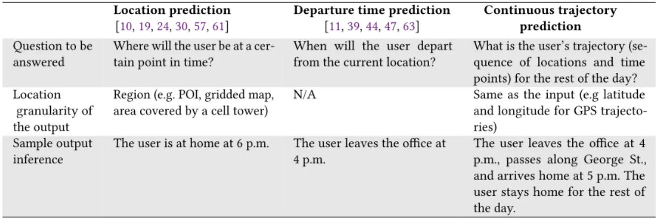
Table 1. Comparison between Location prediction, departure time prediction, and our problem (continuous trajectory prediction)

Location prediction

[10,19,24,30,57,61]

Departure time prediction

[11,39,44,47,63]

Continuous trajectory prediction

Question to be answered

Where will the user be at a cer-tain point in time?

When will the user depart from the current location?

What is the user’s trajectory (se-quence of locations and time points) for the rest of the day? Location

granularity of the output

Region (e.g. POI, gridded map, area covered by a cell tower)

N/A Same as the input (e.g latitude

and longitude for GPS trajecto-ries)

Sample output inference

The user is at home at 6 p.m. The user leaves the office at 4 p.m.

The user leaves the office at 4 p.m., passes along George St., and arrives home at 5 p.m. The user stays home for the rest of the day.

research and is mentioned in the table. Table1also illustrates the sample outputs for a typical scenario. Assume that the user is at the office at 3 pm and wants to buy groceries on his way home from the office. What location prediction and departure time approaches can contribute to a recommendation system is to advise the departure time (i.e. 4 pm) and the location at 6 pm (i.e. home). Predicting the user’s location, the recommendation system suggests only places near the home or office for shopping. However, having the trajectory of the user between the office and home, the recommendation system can also suggest the closest shops on the route home for the user. It can also check if that shop is open at the time the user will reach the shop.

Despite its importance to applications, none of the existing works has focused on the completion of a partial daily trajectory of a user while predicting spatial and temporal sequences with fine granularity for both labeled and geographical trajectories. Routing and traffic recommendations would greatly benefit from such an approach. For example, assume that the user is on her way to work in the morning. By predicting the path to the office and the departure time, a location-based service provider could notify her of transport disruptions in advance and suggest alternative routes with added precision. A short summary of our approach starts with a user’s trajectory up to a certain time of the day. Our algorithm predicts the trajectory for the rest of the day. For example, we have a trajectory for the morning (e.g. up to 12:00) and the problem will be to predict the trajectory in the afternoon (e.g. from 12:00 to 23:59). We predict a trajectory which includes the sequence of future locations with time stamps that will be visited by the user for the rest of the day. If the trajectory is a geographic one, e.g. GPS locations, then the granularity of the prediction is at the GPS level rather than, like in other approaches, with a coarser granularity of regions [56].

Methodologically, our approach investigates the similarities between the given sub-trajectory of the current day and the historical data for prediction. Specifically, the trajectories from the historical data similar to the given sub-trajectory play an important role in the prediction of the succeeding part of the new day’s trajectory. For example, it may be inferred from the historical data that if a user goes to university early in the morning, she would leave the university early. Therefore, if the trajectory in the morning shows that the user goes to university early, a reasonable prediction should anticipate that the user does not stay at the university for a long time. Practically, we are solving a discrimination task by selecting a past afternoon trajectory according to the similarity of morning trajectories. Therefore, defining a comprehensive similarity metric between the trajectories is essential in the proposed method. To do this, we combine two similarity metrics by considering the spatio-temporal properties of the trajectory as well as the sequence of the locations. We evaluate our method

with bothlabeled trajectoriesandgeographical trajectories, and the results demonstrate the effectiveness and efficiency of the method compared to baselines. Using our method, the prediction error is reduced by 10% and 35% for labeled trajectories and geographical trajectories, respectively. This saves the user’s time and enhances her experience. For example, assume that a recommendation system recommends the user to watch fireworks in the main square at 9 p.m. based on the prediction. However, the user arrives at 8 p.m. and she has to discard the recommendation or wait for one hour. On average, our approach reduces the waiting time to 40 minutes. Similarly, from the spatial point of view, the recommended location might be one kilometer away from the user’s location. Using our method, the distance decreases to around 650 meters.

The main contributions of this paper are two-fold, the problem and the solution, including:

• We propose a novel continuous trajectory prediction problem:Given a user’s initial day trajectory (e.g trajectory in the morning), can we predict the user’s daily trajectory for the rest of the day (e.g. prediction of the afternoon trajectory).

• We introduce a mechanism that combines similarity metrics over temporal sequences of locations to estimate similarity of user trajectories. This new metric provides an effective comparison between two trajectories.

• We complete the partial daily trajectory by predicting the trajectory for the remainder of the day. To ensure the quality of the predictions, different components are deployed in our method, including temporal correlation, temporal segmentation, and outlier removal.

• We apply the method to two real-world datasets consisting of labeled trajectories and geographical trajec-tories, and we show the reduction in the prediction error, which is the difference between the predicted trajectory and the actual trajectory. The considerable decrease in prediction error unlocks more precise spatio-temporal user recommendations in the context of location services.

In the next section, we discuss related work. In Section 3, we formally state the problem. In Section 4, we discuss the rationale behind our approach by leveraging on the salient characteristics of human mobility. Our approach for trajectory prediction is described in Section 5. The experiment results of our algorithm are reported in Section 6. Finally, Section 7 concludes the paper.

2

RELATED WORK

Extensive research has been undertaken on mobility prediction, and it is a key issue in a large number of applications, such as mobile wireless systems [12], road networks [31,33], and smart homes [14]. In the networking community, some researchers focus on prediction in WiFi networks, while others predict the connectivity to GSM mobile phone towers (i.e. CID) [50,62]. These methods anticipate client connectivity to the network to enhance mobility management [42], cell assignment [15], paging [6], and call admission control [69]. In addition to the mobility pattern of smartphone users, trajectory prediction is used in road networks where movements are constrained to roads on the map [31, 33,38]. Location prediction systems are also used in smart home environments to maximize occupant comfort and minimize operation costs [14].

2.1

Human Mobility Prediction

Researchers tackle the human mobility prediction problem in different ways. The main idea is to compare the current pattern with historical data and to find similar patterns for prediction. One way is extracting the frequent trajectory patterns to predict unknown trajectories. Morzy et al. combine two well-known algorithms, PrefixSpan [26] and FP-tree [27], to discover moving rules of objects [49]. Some methods extract the frequent patterns from the historical trajectories of all users in the database and provide a global strategy that works for prediction. The main assumption in these methods is that people tend to follow the crowd in their movements [8,

40,48]. Using the frequent patterns approach alone does not always work, because the user may not follow one of the frequent patterns.

Some approaches combine the idea of global and individual strategies to obtain more predictability in results. Specifically, when the individual predictor does not perform well or is not available due to privacy issues, the global predictor is used [3,10,19,66]. Another approach is to generate theories and models of human routine behaviour and use them for prediction [4,16,30]. The research conducted by Gonzalez et al. shows that human trajectories show a high degree of temporal and spatial regularity, and they modeled the individual travel patterns with a single spatial probability distribution [25]. Calabrese et al. model mobility based on a person’s past trajectory and the geographical features of the visited area to predict the next location [7]. Krumm et al. build a Markov model based on the driver’s long-term trip history from GPS data to predict a driver’s next turn [36]. Ziebart et al. build a model of taxis’ mobility patterns to predict the destination given partially traveled route. Similarly, the authors of [38] use a Bayesian model to model the taxi driver behaviour and predict the destinations. However, both methods are designed to predict the destination, not the route. Our method predicts not only the destination but the trajectory between the current location and the destination.

2.2

Next Location Prediction

Some methods focus on the next location prediction problem, which is a relaxed version of trajectory prediction [10, 18,24,30,31,57]. The next location prediction methods can be classified into two groups according to their prediction method. The first group predicts the location of the user after a specific time,∆, which is specified in each study. For example,∆is 10 minutes and one hour in studies [19] and [61] respectively. Sadilek et al. proposed a model for long-term prediction up to multiple years [54]. In some studies, the effect of∆on performance is investigated [31,57]. Do et al. changed∆to predict a set of locations visited by the user [18]. The second group uses methods that do not take into account the time elapsed, but just focus on the next location that the user goes to, whether it is after a short or a long time [22,24]. In both groups, the GPS coordinates are quantized into cell grid, and the output of the prediction is a cell rather than GPS coordinates.

Some approaches take advantage of other contextual factors to improve the performance [13,17]. For example, Domenico et al. improve the accuracy of the prediction by considering traces of multiple users and show the correlation between the trajectories which can be a signal of social interaction [17]. Next location prediction approaches mainly focus on making predictions at fixed and short time-scales, while our approach predicts the entire remainder of a person’s day.

2.3

Machine Learning Models

Predicting one location among a set of finite locations (e.g., POIs, cells in a gridded map) makes the trajectory prediction problem similar to a classification problem. In this case, the locations are considered as the classes, and machine learning classification techniques are used for the next location prediction [1,38,65]. Krumm et al. propose Predestination to predict drivers’ destinations by producing a probabilistic map of destinations via Bayesian inference [38]. Anagnostopoulos et al. consider visited locations as the feature vector, and then evaluate three classification methods [1]. Tran et al. extract the semantics of the visited locations and use them as the features for a classification tree [65]. To predict the next location within a smart building, Petzold et al. evaluate five machine learning approaches including Dynamic Bayesian Network, Multi-layer Perceptron, Elman net, Markov predictor, and State predictor [51]. In [19], the performances of machine learning models such as Random Forest, Linear Regression and Logistic Regression for predicting 10 semantic location labels are compared in both personalized and user-independent modes. The more relaxed problem is occupancy detection, in which the number of the classes is two [37,58]. Classification models cannot be directly applied to GPS data to predict

coordinates that consist of continuous values. On the other hand, our method is able to predict the continuous values such as the latitude and longitude of the locations.

Recently, deep learning has become very popular. However, to perform representation learning with deep learning require large datasets, as argued by Hu et al. [29], existing representation learning (eg for face recognition) with deep learning is usually trained with millions of data samples. They proposed a novel approach to perform representation learning with small data, which is 10,000 samples. The features that can be extracted from image data are very rich. Daily trajectory data is very small, in comparison to image, audio, text logs, or similar data that has been used in deep learning benchmarks and experiments.

More recent work on next location prediction on geographical trajectories are based on Recurrent Neural Network (RNN) architecture [21,35,43]. The problem is largely focused on using histories of locations visited in the past to predict the next location. This still requires large training samples. Unlike observed this problem, in those papers, each visited location history is an instance. In our case, each day is a sample instance in our historical data, and for each user, there can only be around 30 samples if we only have a month history, and up to 365 samples if a user’s trajectory is logged for up to a year.

2.4

Markov Models and Discretized (grid-based) Approaches

In the literature, one of the common approaches for addressing the location prediction problem is the Markov model [2,10,19,22,24,45]. The difference between Markov-based approaches is the way that the states are defined. For example, for GSM data, the cell towers are considered as states, while for WiFi data, WiFi access points are Markov model states [70]. In a smart environment, proximity to a sensor can be considered as a state [51]. Unlike those using fixed sensors, approaches using GPS data apply a prior spatial discretization (i.e. vector quantization). Some approaches simply use fixed grid on the spatial space [8,48,49], while others extract significant locations by clustering spatially or temporally [3,10,40]. For example, Ashbrook et al. first, cluster GPS data points to find significant locations and then use Markov model to predict the user’s movement from one significant location to another [3]. Banovic et. al use a Markov Decision Process (MDP) framework to model routine behavior described as the user’s daily commute. In the first step, the location logs, including latitudes, longitudes, and time stamps, are converted into states and actions representing the user’s mobility for each day. The states indicate the day of the week, the hour of the day (0-24), the location of the user, and whether the user left, arrived, or stayed at the location for the past hour. The state transition probabilities are modeled with a stochastic MDP to consider the environment’s influence on arrival time (e.g. travel distance, traffic) [4].

Using Markov models for the trajectory prediction problem has two weaknesses. First, only the last location visited by the user is taken into account for the prediction of the next location. Some approaches use different orders of Markov models to obtain better accuracy [3,10]. Second, the output of a Markov model is limited to the states representing a significant location, point of interest, CID, or any labeled location. Therefore, the Markov model is not applicable to GPS data unless a prior spatial discretization is applied (e.g using a gridded map), and this reduces the granularity of the predicted locations. The discretization stage may use density-based clustering techniques to detect significant locations, stay points, or points of interests (POI) [8,49]. The discretization, on one hand, reduces the complexity of the problem and increases the certainty of the results. On the other hand, it also reduces the precision of the approach due to the coarse granularity of the regions. As a result, predicted locations could include several important locations which are common in crowded cities where buildings are in close proximity to each other. For example, if the office and home are located in the predicted region, the location-based service cannot distinguish when the user goes to the office.

TPattern [48] is another example of a grid-based approach. The algorithm is a search tree of the next location within certain time interval in the given spatial and temporal thresholds or resolutions. TPattern requires temporal and spatial density threshold, and the algorithm discretized the working space through a regular grid with cell

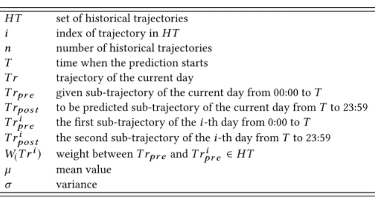
Table 2. Definitions of symbols

HT set of historical trajectories

i index of trajectory inHT n number of historical trajectories

T time when the prediction starts

T r trajectory of the current day

T rpr e given sub-trajectory of the current day from 00:00 toT

T rpos t to be predicted sub-trajectory of the current day fromTto 23:59

T ri

pr e the first sub-trajectory of thei-th day from 0:00 toT

T r_{pos t}i the second sub-trajectory of thei-th day fromTto 23:59

W(T ri) weight betweenT rpr e andT rpr ei ∈HT

µ mean value

σ variance

size set by the user. For example, the experiment in the paper was configured to discretize the GPS trajectories to cells with resolutions of 100 meters, and within 200 seconds. TPattern is also very sensitive to the parameter setting of the spatial thresholds and temporal thresholds. This means it cannot be applied to our problem that looks for the set of consecutive location and time point within any resolutions, without requiring any thresholds, and it is not applicable at all for labelled trajectories.

Compared to the Markov models or grid-based approach used for location prediction, our method can be used to predict the next transition time in the trajectory and the location at any particular time. Furthermore, there is no need for discretization in our method, which results in fine granularity.

2.5

Summary of Gaps

This work addresses human mobility prediction across a day. Existing approaches do not make use of the rich information contained in the previous part of a user’s daily trajectory. Unlike the other methods that predict the destination only, our method predicts the trajectory to the destination using spatio-temporal points. We believe this is vital for an effective location-based service. With trajectory prediction, we investigate not only where will the user be in the future but also how the user gets to that location and when. There is no state-of-the-art method, neither ML techniques, nor trajectory prediction solution, that tackles the same problem.

Our proposed algorithm works with both GPS trajectories(lat, long, timestamp), and labelled or symbolic trajectories(location label, timestamp). The latter is important, as there are large logs of data from cell towers, WiFi access points, Bluetooth beacons, and also Places of Interests, location-based social media check-ins etc. with only location labels or identifiers, without actual location information. Existing trajectory prediction algorithms are not usually applicable to labelled trajectories as they often involve distance based computation, which cannot be performed on labelled trajectories without any exact location information. Therefore, most problems (and solutions) that deal with labelled trajectories are focused on next location prediction at the next look-ahead time with a predefined time window or temporal resolution.

By obtaining this information, the user can be notified about the consequence of her movements in advance. In this way, a location-based system alerts the user about events that may happen during the trip to the destination.

3

PROBLEM DEFINITION

In this section, after introducing the notations, we define the problem. Table2lists the symbols used in this paper.

Definition 3.1. Atrajectoryis a trace of locations, represented by a series of chronologically ordered points,

0 10 20 30 40 50 0 10 20 30 40 50 Afternoon similarity Mor ning similar ity

(a) Device Analyzer dataset (b) MDC dataset

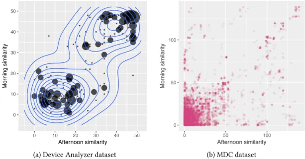
Fig. 1. Correlation between the trajectories in the mornings and in the afternoons

p1,· · ·,pi,· · ·,pm >=<(loc1,t1),· · ·,(loci,ti),· · ·,(locm,tm)>. For geographical trajectories, such as for GPS data,locis a geospatial coordinate set; in labeled trajectories, e.g. a sequence of Cell IDs of WiFi Access points,

locis the label assigned to a location.

Definition 3.2. The historical trajectories of the user containingndays of data isHT =T r1, ...,T rnwhere

T ri denotes the trajectory of the user during thei-th day. A day starts at 0:00 and ends at 23:59.

Definition 3.3. Current dayis the target day when the prediction takes place. The trajectory of the current day

isT r.

Definition 3.4. Prediction time(T) is the time of the current day when the prediction starts.

Definition 3.5. T ri

pr eis the first sub-trajectory of thei-th day that is from 0 : 00 toT whileT rposti is the second

sub-trajectory ofi-th day that is fromT to 23 : 59. For the current day, the sub-trajectory from 0 : 00 toT isT rpr e

and the sub-trajectory fromT to 23 : 59 isT rpost.

The definitions of the symbols are listed in Table2. Given these definitions, we can now define our problem statement.

Problem:Given the historical trajectory,HT, and the user’s initial trajectory of the current day,T rpr e, our

problem is the prediction of the continuous trajectory for the rest of the day,T rpost.

4

OBSERVATIONS IN HUMAN DAILY TRAJECTORY

In this section, we discuss the rationale behind our approach by discussing three observations, each of which is examined on data described in the following subsection.

50 55 60 7 14 21 28 ∆ DTW 6 8 10 7 14 21 28 ∆ DTW

(a) Device Analyzer dataset (b) MDC dataset

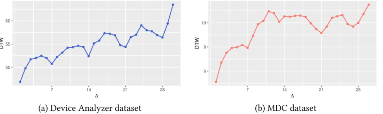
Fig. 2. Temporal correlation between the trajectories that have∆days difference

4.1

Data Description

To validate the observations, we evaluate two types of datasets: a labeled dataset (Device Analyzer) and a geographical dataset (Mobile Data Challenge). We use these same two datasets for our subsequent experiments. • Device Analyzer: The Device Analyzer app gathers data about running background processes, wireless connectivity, GSM communication, and some system status and parameters. In this dataset, MAC addresses, WiFi SSIDs, and other forms of identification are hashed due to privacy purposes. Therefore, there is no ground truth or information about the geography or semantics of the locations. The trajectories consist of labeled cell tower IDs (CID), and the sampling rate is every 15 minutes. This makes the trajectory length equal to 96 for one day. In our experiments, we consider 225 users who have more than 40 days of data. For each user, we apply our approach to the last 10 days [67].

• MDC dataset: The Mobile Data Challenge (MDC) dataset provides geolocation information for nearly 200 users. In addition to GPS data, WLAN data is also used for inferring user location. The location of WLAN access points was computed by matching WLAN traces with GPS traces during the data collection campaign. As an adequate amount of data is needed for prediction, we exclude users who do not have enough data and only considered users with more than 40 days of data. 136 users satisfy this condition. Similar to Device Analyzer dataset, we process the same amount of data (i.e. 10 days) for each user and RMSE is reported over all instances [34].

The Device Analyzer data provides hashed cell tower IDs (CIDs) and we call it thelabeledtrajectory dataset trajectory, composed of CIDs and time stamps. The MDC dataset provides the geographical location of the user and the trajectories include latitude, longitude, and time stamps and we call it thegeographicaltrajectory dataset. WhenT is 12 : 00, the trajectory of a day is split into morning and afternoon sub-trajectories.

4.2

Observation 1: Positive Correlation Between the Morning and Afternoon Sub-trajectories

Figure1shows the scatter plot for similarities in the mornings and in the afternoons measured by Dynamic Time Warping (DTW). (We explain later how we apply DTW to our labeled and geographic datasets.) In Figure1a, each of the 2000 points represents 2 random days taken from the same user in the labeled dataset. The vertical axis represents the morning DTW difference of the two days, and the horizontal axis represents the afternoon DTW difference, where a smaller difference indicates higher similarity. Since this is labeled data, the DTW differences

are integers ranging from 0 (high similarity) to 48 (high difference). The strongest cluster in this plot is centered around (10,10). This indicates that days that are relatively similar in the morning and also relatively similar in the afternoon. Exact matches are rare, hence there are no points at (0,0). The size of each point is proportional to the number of points occupying that coordinate.

Figure1b shows the same analysis for 2000 random pairs of days in the geographic dataset, where the DTW difference is a continuous value. We again see a large cluster near (0,0). Taken together, the plots in Figure1 imply that if two trajectories are similar in the morning, it is expected that they are similar in the afternoon, too. This validates the first observation. For example, if someone works for two companies and has two routines, the morning trajectory often identifies which routine will be followed in the afternoon. We make use of this observation by predicting a person’s afternoon trajectory based on their morning trajectory

4.3

Observation 2: Positive Temporal Correlation

The importance of each historical trajectory varies and depends on its date. To show the date effect, 2000 random trajectory pairs are selected from each dataset. Each trajectory pair includes two trajectories from two days with less than 30 days gap from the same user. Figure2shows how much the closeness of the dates reflects the similarity between two trajectories, where similarity is again measured by DTW. Specifically, thex-axis indicates the gaps (∆) in days between the dates of two trajectories, while they-axis reflects the average similarity. It is observed that 1) overall, as∆increases, the similarity decreases, and 2) when∆=7, the weekly periodicity

appears, which means trajectories are more similar between two days with 7 days difference. Thus, in general, the closer the date of a historical trajectory to the current prediction date, the more important it is. The reason is that people often have a similar routine in two close days (e.g. two consecutive days) [13]. This temporal correlation indicates that higher priority should be given to the trajectories with the closer dates or dates that are one week apart. For example, for prediction of Monday mobility, this observation implies that it is better to use the trajectory of the last Monday rather than the trajectory from the last Tuesday. We use the temporal correlation to compute weights on each previous day to use for predicting the current day. Days with higher correlation are given more weight.

4.4

Observation 3: Outlier Trajectories

There are outlier trajectories, which are different from people’s normal routine (i.e. visit to a location by exception) and which are unlikely to happen again (especially considering the entire trajectory as a whole). Then, when making trajectory predictions, these outlier trajectories should be excluded. Here, we elaborate one example to clarify the effect of outlier removal stage. Assume that the user has a strict routine on Wednesdays and we want to predict the afternoon trajectory given a Wednesday morning trajectory. The temporal correlation specifies to pick the afternoon trajectory of the last Wednesday because it is the closest day to the current day with similar morning trajectory. Now, assume that on Wednesday afternoon last week, the user deviated from his routine to visit a new location (e.g. visiting a friend in a hospital) and this visit had never been repeated in the historical data. Observation 3 implies that such a visit was temporary and unlikely to happen again. In other words, the predicted trajectory should not be nor include an outlier.

In summary, the proposed method is based on the above observations. 1) We predictT rpost using the historical

trajectories that have the sub-trajectories similar toT rpr e. 2) We calculate temporal correlation to give priority

the historical trajectories based on their relative date. 3) The historical trajectories that include outliers are not used for the prediction.

Measuring DTW similarities between Trpreand Trprei

0θiθn

Measuring ED similarities between Trpreand Trprei

0θiθn

Updating DTW similarities based on ρ and temporal

correlation Finding temporal correlation between trajectories Normalizing Temporal segmentation for the afternoon

Finding the subǦtrajectory in each segment and

linking them

Removing the outlier subǦ trajectories in each

segment Updating ED similarities

based on ρ and temporal correlation Normalizing

a

b

c

d

e

f

Computing n*ndistance matrix between historical trajectories

in each segment Historical Trajectories HT Current day day 1 . . day n TrMo TrAf=? Tr1 . . Trn Trpre Trpost Trpre1 Trpost1 Trpren Trpostn . . . . Output: Trpost

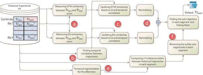
Fig. 3. Diagram of the approach to continuous trajectory prediction

5

CONTINUOUS TRAJECTORY PREDICTION

In this section, we provide an overview of the proposed approach to partial human daily trajectory prediction, as shown in Figure3:

(a) The first stage is to compareT rpr ewithT rpr ei , the morning sub-trajectories from the historical trajectories.

The goal is to weight the historical trajectories based on their similarities toT rpr e. Two similarity metrics

are deployed in our approach: Dynamic Time Warping (DTW) [32] and Edit Distance(ED) [9]. We will describe these metrics later in the section.

(b) The temporal correlations are processed to quantify the impact of date differences on the prediction. (c) Together with (a), the temporal correlation betweenT rpr eandT rpr ei are used to enhance the corresponding

importance ofT rpr ei . For example, the afternoon trajectory of yesterday might receive a higher weight

compared to the afternoon trajectory of a day from last month.

(d)The two similarity measures (DTW and ED) are normalized in this stage. After normalizing the similarity measures, they are combined to form the final weight of each historical trajectory. The final weights indicate the similarity of the morning parts of the historical trajectories toT rpr e. The afternoon part of the

trajectories that received high weights will be used for prediction in the final stage.

(e) A temporal segmentation method [55] is deployed on the historical afternoon trajectories. Then, the prediction is performed within each segment. Ideally, each temporal segment represents the period over which an activity is undertaken. For example, if the user often goes for lunch between 12:00 and 13:00, [12:00, 13:00] is one of the temporal segments.

(f) In each afternoon segment, a distance matrix is built. The distance matrix indicates the distance/similarity between two sub-trajectories in the historical data during that segment. Based on the distance matrix, we discard the outlier sub-trajectories that represent the trajectories that are unlikely to happen during the current day. From the rest of the trajectories, we choose the sub-trajectory of a day with the highest weight assigned in stage (d). The predicted sub-trajectory are linked together to formT rpost.

We detail each of the above components in the following sections, including trajectory similarity metrics, temporal correlation, temporal segmentation, and outlier removal.

ED similarity measure 5/02/2012 10/02/2012 15/02/2012 20/02/2012 5/02/2012 10/02/2012 15/02/2012 20/02/2012 Very similar Very different

Fig. 4. Similarity matrix for 20 successive days. The darker the cell, the stronger the similarity.

5.1

Similarity Metric

There are several metrics to measure the similarity between two trajectories. For example, the four most common metrics are Fréchet Distance, Dynamic Time Warping (DTW), Longest Common Sub-Sequence (LCSS), and Edit Distance (ED), all of which have been introduced and compared by Toohey and M. Duckh [64]. Of these metrics, DTW relies on matching points in trajectories. Specifically, a single point in one trajectory can be matched to multiple points on the other trajectory based on the distances. The calculation of distances between the points is performed using a chosen distance function. For labeled trajectories, the distance function only checks whether the two labels are equal or not. If the two labels match, the distance is zero. Mismatched labels have a distance of one. For geographic trajectories, the distance between points is the great circle distance measured from the two latitude/longitude pairs. DTW considers delays in the trajectories. This means that similar sub-trajectories are matched together even though their timestamps are different. However, outliers can significantly affect DTW because there has to be a match between every point in both trajectories [64]. ED aims to count the minimum number of edits needed to make two trajectories equivalent. This means after the edits all of the locations in the trajectories have to be the same. For geographical trajectories (i.e. MDC dataset), we consider two locations as the same location if they are within 0.1 range in latitude and longitude. Among different variations of edit distance, we use the one described by Chen et al. [9]. ED compares the trajectories in every fine-grained time slot and does not consider delays in the trajectories. ED is more robust in the treatment of outliers than DTW.

As the similarity metric plays a critical role in our approach, we propose a metric that integrates DTW and ED together to provide a comprehensive similarity measure. This is reasonable, because 1) Fréchet distance and DTW are highly correlated (R=95%); 2) LCSS and ED are highly correlated (R=83%) [64]. Furthermore, DTW and ED

are compatible with non-geographic (labeled) trajectories such as trajectories represented by cell tower IDs. Figure4shows the similarity matrix over 20 successive days using DTW based on the Device Analyzer (labelled) dataset. Specifically, each entry denotes the similarity value between trajectories in two days. It is observed that days 17-20 are very different from the other days. The user may have gone for a trip in that period to visit new places in other cities. And the calendar shows that this period is from Friday to Sunday, which strengthens this hypothesis.

5.2

Weighting Historical Trajectories

Here, we specify how we combine DWT and ED with the observed temporal correlation between trajectories. GivenT rpr e, its DTW similarity toT rpr ei ∈HTis defined as follows:

WDT W(T ri)=DTW(T rpr e,T rpr ei ) ×TcorDT W(∆), (1)

whereTcordenotes the effect of the temporal correlation in the weighting.∆denotes the difference between the

dates whenT rpr eandT ri happened. To calculateTcor(∆), we use the historical trajectories to find the correlation

between the trajectories with∆days difference. Here, we are emphasizing the effects of Observation 2 that∆is an important factor governing the similarity between days based on how far apart they are in time." Similarly, the ED similarity is defined as follows:

WE D(T ri)=ED(T rpr e,T r_{pr e}i ) ×T_corE D(∆). (2)

Small values ofWDT W(T ri)andWE D(T ri)mean that theT rpr eandT rpr ei are similar. According to Observation 1,

among the historical trajectories, ones that are most similar toT rpr ein the morning should get higher weights

when predicting the afternoon trajectory.

5.2.1 Normalization._{Before summing up the ED and DTW similarity values, they are z-normalized. That is,}

each type of similarity values has zero mean and a variance of one. This provides a comprehensive similarity measure that plays a critical role in our approach.

W(T ri)=WDT W(T r i_{) −µ} DT W σDT W + WE D(T ri) −µE D σE D , (3)

whereµandσdenotes the mean and variance that are calculated for each user separately, and they are based on the user’s historical data.W()is the total weight assigned to a historical trajectory considering ED and DTW metrics and temporal correlations.WDT W_σ(T ri)−µDT W

DT W and

WE D(T ri_{)−µE D}

σE D are the normalization for DTW and ED,

respectively. This normalization is introduced to remove the scale effects and gives both metrics an equal priority.

5.3

Temporal Segmentation

Factorizing a time period into several temporally homogeneous segments is called temporal segmentation. Considering trajectories from a user, temporal segmentation reveals the departure times when the user changes her activities. For example, assume one leaves home at 7 am, works at the office from 9 am to 4 pm, and then goes outdoors until 6 pm every day. In this example, 7am, 9am, 4pm, and 6pm are the departure times and [7am-9am], [9am-4pm], [4pm-6pm], and [6pm-7am] are the temporal segments .

To predict the trajectory of the user in the afternoon, a temporal segmentation method is applied to historical trajectories to find the usual changes in the user’s daily activities, such as when the user usually goes from home to work. Then, a sub-trajectory is predicted for each segment. Temporal segmentation allows us to analyze fine-grained segments and discard the outlier sub-trajectories in each segment.

We use the Information Gain Temporal Segmentation (IGTS) introduced in [55]. IGTS computes the distribution of the user’s locations in each segment and tries to capture the segments that have the lowest entropy. Low-entropy segments imply that the user’s location is predictable in that segment. For example, [12am-6am] is a low-entropy segment for a common user because the user is probably at home during this period. If the trajectories contain geographic locations, before using IGTS, the locations should be quantified (e.g by using gridded map). To find the number of the segments, IGTS uses a formula to choose the best candidate from a range of numbers based on knee-point detection [55]. If the number of the segments is too large, the predicted trajectory will have a high variation. Therefore, we select the best candidate for the number of segments ranging from 2 to 6. The temporal segmentation method is applied per user. This makes the method highly robust to individual habits and routines.

Tr1 _{. . . Tr}n Tr1 _{. . . Tr}n Tr1 _{. . . Tr}n _Tr Tr Tr Historical Trajectories Current Day Instance 1 Instance 2 Instance 3

Fig. 5. Three sample instances from one user. Each block represents one day.

5.4

Outlier Removal

In this stage, we discard the historical trajectories that have abnormal sub-trajectories in the afternoon. According to Observation 3, these trajectories are discarded because it is unlikely to have a sub-trajectory similar to the abnormal sub-trajectories. The abnormal sub-trajectories are sub-trajectories that are not found in the historical data such as going to the airport to pick up someone, visiting a friend in a hospital, or inspecting an apartment to buy. The outlier removal stage is done regardless of similarities in the morning parts. This means we discard the historical trajectories with abnormal sub-trajectories in the afternoon even if the morning parts are similar to the current day.

To remove the outliers, we build a distance matrix for each afternoon segment results from temporal segmenta-tion stage (e.g. from 1 pm to 4 pm). The distance matrix,DS1, is ann×nmatrix whereDS_{i j}1denotes the distances between the sub-trajectoriesi andjin segmentS1. We use DTW to compute the distance matrix. An outlier

sub-trajectory is based on its closest neighbour (the most similar sub-trajectory). If the closest distance is higher than a threshold, the sub-trajectory is considered as an outlier. The outlier removal is performed in each segment independently.

5.5

Linking Trajectories

Finally, we make the prediction for each segment obtained from the component of temporal segmentation, then link these predictions together to form the prediction ofT rpost. Namely, the corresponding segment in T r_posti ∈HT with the highest weightW(T ri)is selected as the prediction for each segment inT rpost. Then, we

naturally link the predictions for each segment together to make the prediction forT rpost.

6

EXPERIMENTS

Before evaluating the effectiveness of the proposed method thoroughly, we clarify the experiment setting. For each user, we pickmconsecutive days of trajectories (m>n), wherendenotes the size of historical trajectories used for the prediction of one day afternoon trajectory. For each day, we run our approach while considering the pastndays as the historical data, using the (n+1)-th day as the first test trajectory. Based on the morning trajectory (i.e. the given part of the trajectory of the current day), we predict the afternoon part of the (n+1)-th day. For the next day, again, we predict the afternoon trajectory based on the pastndays and the morning trajectory of that day. We continue the prediction of the afternoon sub-trajectories for each day until we reach them-th day. Therefore, we have(m−n)test instances for each user. In other words, each day of data is treated as a test instance. Figure5shows three sample instances from one sample users’ trajectories.

For each instance, the predicted trajectory is compared to the actual trajectory and the error is calculated using DTW. The prediction error shows how much the predicted trajectory is similar to the actual trajectory. If

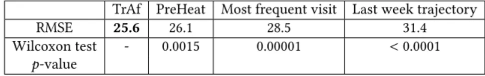
Table 3. Tests show that our algorithm’s mean performance is better than the baseline algorithms on the Device Analyzer dataset by a statistically significant margin

TrAf PreHeat Most frequent visit Last week trajectory

RMSE 25.6 26.1 28.5 31.4

Wilcoxon test - 0.0015 0.00001 <0.0001

p-value

the predicted trajectory is exactly the same as the actual trajectory, DTW returns zero. Otherwise, the error is the DTW distance between the two trajectories. DTW is an effective way to evaluate the prediction, because it accounts for both the spatial and temporal differences between the prediction and the actual trajectory. Calculating the error for each instance, the Root Mean Square Error (RMSE) is reported for all data. Specifically, RMSE is the root mean square of the prediction errors measured by DTW. For the labeled trajectories, we also report precision and recall in addition to RMSE. However, it should be noted that precision and recall only consider the set of the predicted locations and do not consider the sequence and transition times. In the experiment results, our method is denoted by "TrAf".

6.1

Baselines

For comparison, we use the following baselines:

• Last week trajectory: According to Section4.3, of the historical trajectories, one of the most similar trajectory toT rpost is the trajectory of the afternoon of the last week. We use this as our first baseline. This

baseline is similar to "Same place" baseline used in the next location prediction methods [18].

• Most Frequent visit: This baseline finds the most visited locations at each time of the day. For example, for finding the location at 1 pm, the method searches for the location in the historical trajectories that is most often visited at 1 pm [18,19].

• PreHeat: This algorithm was designed for the problem of occupancy detection. Specifically, given the historical records and the morning occupancy, PreHeat predicts the occupancy in the afternoon. To this end, this method detects 5 days that have the most similar occupancy patterns to the current day in the morning and then, the probability of the occupation is calculated based on the detected days. Please note that since there is no state-of-the-art method that tackles exactly the same problem addressed in this paper, we chose

PreHeat, a state-of-the-art-method targeting originally a different problem (i.e. occupancy detection) as a

baseline comparison, as this has some similar characteristics which allow some level of comparison. We adapt PreHeat to make it applicable to our data. For labeled trajectories, we consider one day instead of 5 days because it is not possible to calculate the mean value of labels. For geographical trajectories, the mean values of the latitude and longitude are considered as the coordinate of the predicted location. We also evaluate the algorithm when the number of the detected similar days is 10 [58].

• Markov model: It is one of the most popular approaches for mobility prediction problem [2,10,19,22,24, 45]. However, Markov models cannot be applied directly to the GPS data and there should be a discretization stage for defining Markov states. In our implementation, we use a grid map for discretization, and each cell is considered as a state.

6.2

Experiments on Labeled Trajectories

In this experiment, we predict the labeled afternoon trajectories of 2250 days from 225 Device Analyzer users (10 for each user). The length of the historical data is 30 days, i.e.n=30, which means for prediction of the afternoon

0 10 20 30 40 50 TrAf PreHeat

Most frequent vist Last w eek tr ajector y Similar ity (DTW)

Fig. 6. Results for 2250 instances from the Device Analyzer(labeled) dataset.▲denotes the mean value. Table 3 shows the

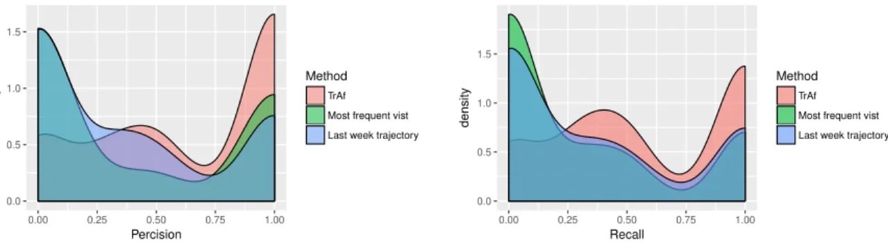
difference is significant. 0.0 0.5 1.0 1.5 0.00 0.25 0.50 0.75 1.00 Percision density Method TrAf Most frequent vist Last week trajectory

0.0 0.5 1.0 1.5 0.00 0.25 0.50 0.75 1.00 Recall density Method TrAf Most frequent vist Last week trajectory

Fig. 7. Distribution of precision and recall of predicting the full set of locations of the whole day (Device Analyzer dataset). The temporal aspects of the errors are not considered in this experiment.

previous 30 days. Here,T is 12 pm which means we have the trajectory of the current day up to 12 pm and trajectory between 12 pm and 12 am is unknown. This makes the lengths ofT rpr eandT rpost equal to 48. The

impacts of the prediction time and size of historical trajectories are investigated in the following subsections. In Figure6, the y-axis denotes the similarity between the predicted trajectory and the ground truth. The box plot containing inter-quartile range (IQR), a measure in descriptive statistics. The IQR is the 1st quartile (25%) subtracted from the 3rd quartile (75%). The box demonstrates the values between 1st quartile and 3rd quartile while whiskers extend to data within 1.5 times the IQR. The median is also shown in the box. The maximum error is 48 and this happens when none of the predicted Cell tower IDs (CIDs) is the same as the actual CIDs. The

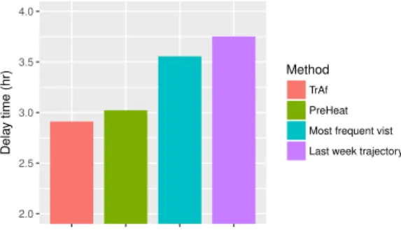
2.0 2.5 3.0 3.5 4.0 Dela y time (hr) Method TrAf PreHeat Most frequent vist Last week trajectory

Fig. 8. Average error in predicting the departure times (Device Analyzer dataset). The spatial aspects of the errors are not considered in this experiment.

Table 4. Tests show that our algorithm’s mean performance is better than the baseline algorithms on the MDC dataset by a statistically significant margin

TrAf TrAf TrAf PreHeat PreHeat Most frequent Last week

(Excl. OR) (Excl. OR & TS) (5 days) (10 days) visit trajectory

RMSE 6.3 7.5 7.6 8.6 10.1 13.0 14.7

Wilcoxon test - <0.0001 <0.0001 <0.0001 <0.0001 <0.0001 <0.0001

p-value

figure shows that the trajectories predicted by our method are more similar to the actual trajectories. To show that this superiority is not by chance, a statistical analysis, Wilcoxon test, is conducted. RMSE and thep-values are reported in Table3. All the tests show our algorithm’s mean performance is better than the baselines’ means to the 0.0001 significance level.

It can be seen that the variation of the result is high and the certainty of all methods are low. The reason is that the human mobility has some limits for prediction and it is not completely predictable [61]. In fact, it is likely to see new trajectories that are different from the historical trajectories. For example, the user may leave the office earlier, or she may catch up with her friends after the working hours.

The reality is that the performance of each method depends on the user’s behaviour. For example, if morning trajectories and afternoon trajectories of a user are highly correlated then our method works better. For users that have strict routine over a week, the trajectory of the last week is an appropriate estimation for today’s trajectory compared to other methods. However, our method has the best result on average.

In addition to DTW, which considers temporal and spatial aspects at the same time, we conduct temporal and spatial evaluation separately. For spatial evaluation, we report the distribution of precision and recall in Figure7. To calculate precision and recall, the set of predicted locations is compared to the actual locations visited by the user. Clearly, the temporal aspects such departure time are not considered. For temporal evaluation, we report the difference between the actual and predicted first departure time after 12 p.m. Figure8shows the results. It can be seen that our method outperforms the baselines in both experiments.

0 2 4 6 8 TrAf

TrAf (Excl. OR) TrAf (Excl. OR & TS)

PreHeat (5 da ys)

PreHeat (10 da ys)

Most frequent visit Last w eek tr ajector y Similar ity (DTW) 0.0 0.2 0.4 0.6 0.8 0 1 2 3 4 5 Similarity (DTW) Distr ib ution Method TrAf PreHeat (5 days) Most frequent visit

(a) (b)

Fig. 9. (a) Box plots for the baselines and different settings of our approach. y-axe shows the similarities between the predicted trajectories and ground truths.▲: mean value, OR: Outlier Removal, TS: Temporal Segmentation (b) Distributions of the

similarities for three methods

6.3

Experiments on Geographic Trajectories

From the MDC dataset, all the users with more than 40 days data are chosen for evaluation (136 users). The size of the historical trajectory is 30 days in this experiment, i.e.n=30. The total number of test instances is 1360 (10 for

each user). For each instance, we measure the similarity between the predicted trajectory and the ground truth. Figure9(a) shows the box plot. For each method, the▲indicates the mean value while the box plots report

inter-quartile ranges (IQR). To show the impact of Temporal Segmentation (TS) and Outlier Removal (OR), we run our method with and without these stages. The results indicate the positive impact of TS and OR. Figure9(b) shows the distributions of the DTW distance between the actual and predicted trajectories, where we can see that the trajectories returned by our method are closer to the ground truths with higher probabilities of low DTW.

The RMSE of our method is 35% less than the best baselines, which has a significant impact on the level of accuracy that location service recommendation can achieve and therefore on the user experience. Similar to other experiments, we evaluate the performance using DTW, which is able to consider both the temporal and spatial deviation. 35% reduction in error means, on average, that the user is 35% closer to the predicted location or the user has to wait for 35% less time for an event to take place. In practical terms, this means that the user spatial and temporal proximity to a recommendedevent(e.g., a show, a train to catch) is more than doubled.

6.4

Impact of Historical Trajectory Size

Here, we investigate the impact of the size of the historical trajectories,n, on the accuracy of the prediction. Specifically, we varynfrom 2 to 60 days with the step length 1 on the Device Analyzer (labeled) dataset. In this experiment, we use three users with a total of 943 days of data ( 467, 221, and 255 for the three users). The RMSE is reported in Figure10.

From Figure10, we can observe that: 1) the last week trajectory approach is not affected because it does not consider the historical trajectories; 2) increasingnmakes the most frequent visits approach more accurate. This trend continues untiln=7, and after that increasing the historical trajectory size makes the approach worse.

The reason is that the user may change behaviour and may not go to the places that she used to go. A long series of historical data causes the most frequent visits approach to promote the locations that have been frequently

30 35 40 0 20 40 60 n R MSE (DTW) Method TrAf

Most frequent visits Last week Trajectory

Fig. 10. Effect of the historical trajectory size on the accuracy of prediction. The performance of our approach improves with increasing the historical trajectory size.

0.0 2.5 5.0 7.5 10.0

2:00 AM4:00 AM6:00 AM8:00 AM_{10:00 AM12:00 PM2:00 PM4:00 PM6:00 PM8:00 PM10:00 PM} T

RMSE

Method

TrAf

Most frequent visit Last week trajectory

Fig. 11. Impact of prediction time on the performance. Having more data from the current day leads to less error (or more accurate prediction).

visited a long time ago; 3) the proposed method handles the size of the historical trajectories well. There are two reasons for this. First, by considering the temporal correlation, we give priority to the trajectories from consequential dates. Generally, closer dates are more consequential. This gives the trajectories from a long time ago less effect. Secondly, our method only uses the historical trajectories that have the similar morning trajectory asT rpr e. Therefore, if the behaviour of the user changes, our method recognizes it by analyzing and comparing

the morning trajectories.

Changingncauses a trade-off between the accuracy and processing time. For a large value ofn, we have accurate results but at the same time, our approach becomes more costly. In our experiment, we setnto a number between 20 to 30, because increasingnmore than 30 does not lead to a significant increase in accuracy.

6.5

Impact of Prediction Time

According to our problem formulation, the current day trajectory of the user up to prediction timeT is known. Here, we investigate the impact of prediction time,T, on the accuracy. To this end, we design the experiments by

2.0 2.5 3.0 0.0004 0.0016 0.0064 0.0256 0.1024 0.4096 1.6384 6.5536 Threshold RMSE

Fig. 12. Impact of the threshold of the outlier removal on the accuracy of prediction. The dashed line shows when there is no outlier removal stage.

varyingTfrom 1 am to 11 pm with a step length of 1 hour, and we use the last 20 days as the historical trajectories, i.e.n=20. In this experiment, the same set of users as Section6.3are analysed. Specifically, the experiment on the

geographic dataset is repeated 23 times (once for eachT). Figure11shows the relationship between prediction accuracy in RMSE and prediction time. It is observed that: 1) the trends are decreasing because DTW returns smaller values for short trajectories; 2) furthermore, when we have more data from the current day, the prediction is more accurate. If the prediction time is after 7 pm, our method and "most frequent visits" overlap, otherwise our method outperforms the baselines; 3) there is a steeper decrease starting around 12 pm in the DTW of our method. This means the trajectories from 11 a.m. to 12 p.m. is very informative and more predictive.

6.6

Impact of Outlier Removal

In this experiment, the effect of the outlier removal stage with different thresholds is investigated. Figure12 shows the impact of the threshold used for detecting outliers on the accuracy of the proposed approach on the geographic dataset. Thex-axis has a logarithmic scale to assist interpretation. When the threshold is too small, a high portion of the sub-trajectories is recognized as outliers. In this case, the error is high because some useful information for the prediction is discarded. By increasing the threshold up to 0.0128, the results improve further. When the threshold increases, fewer sub-trajectories are recognized as outliers. When the threshold is higher than 1.638, none of the sub-trajectories are recognized as outliers and the performance is the same as the approach without outlier removal.

6.7

Experiments on Gridded Map

Here, we compare our method with a first-order Markov model. To run Markov model on the geographic dataset, we use a gridded map to discretize the GPS data. In this case, each state is one of the cells in the gridded map. Consequently, the locations predicted by Markov model are cells rather than geographic coordinates. Figure13 shows the difference between the outputs of our method and the Markov model.

To compare the results, we discretize the output trajectory from our method. To measure the prediction error, we compared distance between the centroid of the predicted and the actual tile in the Markov model. Figure14 shows the effect of the gridded size on the performances of both methods. For large grid sizes, the Markov Model performs better than our method. However, when the grid size is reduced, our method performs better, because the data becomes sparse and there is not enough historical data to build a Markov Model.

(a)

(b)

Fig. 13. (a) Sample output of the proposed approach. The red dashed line shows the predicted trajectory of our method. The black line is the actual trajectory of the user (b) Sample output of the Markov model. The red cells in the gridded map show the prediction of the Markov model.

0.980 0.985 0.990 0.995 1.000 1.005 0.1 0.05 0.025 0.0125 Grid size (MM error)/(TrAf error)

Fig. 14. Comparison between our method and the Markov model for different grid size. The y-axis indicates the ratio between the error of our method and the Markov model. The blue dashed line shows when both approaches have the same performance.

6.8

Comparison with Recurrent Neural Network on Geographical Data

One interesting observation is the efficiency and effectiveness of our proposed method. One may ask ś how does this compare with deep learning? Performing representation learning with deep learning traditionally requires large datasets. As argued by Hu et. al. [29], existing representation learning (e.g. for face recognition) with Convolutional Neural Network architecture is usually trained with millions of data samples. This recent work by Hu et al. [29] claimed to be first to perform representation learning with small data, which is 10,000 samples, with rich features that can be extracted from image data. For some time-series data based problem, small amount of data also does not work well [59,60]. In our case, each day is a sample instance in our historical data, and for each user, there can only be around 30 samples if we only have a month history, and up to 365 instances if a user’s trajectory is logged for up to a year. Trajectory data also does not have as many features as image

Ot-1 Ot Ot+1 Ct-1,ht-1 Xt-1 Ct-1 sigmoid Xt

sigmoid tanh sigmoid

Ct+1,ht+1 Xt+1 ht tanh ht-1 Next unit Last unit

Fig. 15. Architecture of Long short-term memory.

data, requiring re-engineering of the deep learning application. We have previously shown in Figure10that our method has converged at n=30, which means having more than 30 instances do not necessarily reduce the prediction error. Therefore, our hypothesis is that deep learning is not going to work well for our problem.

To test this hypothesis, we implement a Recurrent Neural Network model. This is because many recent works for location prediction using deep learning is mainly based on Recurrent Neural Network (RNN) architecture [21,35,43]. In this instance, we compared our proposed solution with Long short-term memory (LSTM) on geographical trajectories prediction. LSTM is a widely used recurrent neural networks which is capable of learning long-term time dependencies [28]. The architecture of the LSTM is illustrated in Fig.15. Compared with traditional recurrent neural network, LSTM adds four gates to inoperative all cell states. There are three main gates called input gate, forget gate and output gate for input statext, hidden stateht and output state ot, respectively. The other gate is a sigmoid function which is used to modulates the output of these gates. It

perfectly solves the gradient vanish problem in recurrent neural networks.

In this experiment, we used a single hidden layer LSTM since the structure of data is simple. The parameter setting of LSTM is shown in Table5.

Since the computational complexity of neural networks is extremely high, we randomly selected three users and predicted their future trajectories using our proposed methods and LSTM. The experimental setting is as same as the setting in section6.3. We selected 30 days as the training dataset and 10 days as the testing dataset. For each instance, we measured the difference between ground truth and predict trajectories with DTW and calculated the RMSE for each method. We also tried another set of experiment with 60 training days and 10 days

Table 5. Parameter settings for LSTM.

# Hidden Layer 1

# Neurons in the Hidden Layer 32

Number of Features 2

Length of Instance 48

Optimizer Adam

Loss function Mean Square Error

0 20 40 60 80 100 120 140

User1 User2 User3

Users RMS E Methods LSTM (30 samples) LSTM (60 samples) TrAf (30 samples)

Fig. 16. Comparison between our method and the LSTM for three randomly selected users. The y-axis indicates RMSE of our method and the LSTM. We used 30 training samples and 60 training samples for LSTM and only 30 samples for the proposed TrAf method.

testing sample because the performance of the LSTM usually only improves with more training samples. The comparison result is shown in Fig.16.

The experiment results shows that our proposed method is significantly better than LSTM with small sample size regardless of extreme long time training for LSTM. LSTM performs better with more training samples because neural networks heavily rely on the size of the training samples. For the second user, the performance of LSTM with 60 samples is slightly better than the proposed method. However, with the small size of training samples (30 samples), our methods is significantly superior than LSTM in both effectiveness and efficiency on small size training data. We acknowledge the limitation of the LSTM experiments on the small number of users at the moment. We have also not explored fancier techniques in exploring additional mobility features or enriching the trajectory representation, such as with trajectory embeddings [23].Further evaluation is needed to analyze the factors influencing the possible variability of the results.

7

CONCLUSION AND FUTURE WORKS

This paper presents a method for completing the user’s daily trajectory using the initial trajectory of the current day and historical trajectories. The algorithm takes both temporal and spatial aspects into account to investigate the similarities between the sub-trajectories. To improve the performance and reliability of the method, we add some other phases including temporal segmentation, extracting temporal correlation, and outlier removal. The method is applied to the situation where user trajectories are either labeled or geographical. This paper concentrates primarily on the issues of accuracy, and the experiment results show that the proposed method significantly outperforms the state-of-the-art in terms of accuracy and also efficiency. Furthermore, we investigate the impact of different parameters on our method. The high level of precision obtained by the technique has the power to unlock more precise location service recommendations.

Our future works include leveraging other types data in addition to user’s trajectories for improving the performance. For example, in the Device Analyzer dataset, using the context values, such as smartphone logs, sensor data, and user’s activities, could make the prediction more accurate. We will also explore the inherent categories and profiles of user behaviours to explore the predictability across different groups.

ACKNOWLEDGMENTS

The work is supported by the RMIT Sustainable Urban Precincts Program (SUPP) Scholarship and the Australian Research Council’s Linkage Project LP120200305.

REFERENCES

[1] T. Anagnostopoulos, C. Anagnostopoulos, and S. Hadjiefthymiades. Mobility prediction based on machine learning. InMobile Data Management (MDM), 2011 12th IEEE International Conference on, volume 2, pages 27ś30. IEEE, 2011.

[2] A. Asahara, K. Maruyama, A. Sato, and K. Seto. Pedestrian-movement prediction based on mixed markov-chain model. InProceedings of the 19th ACM SIGSPATIAL international conference on advances in geographic information systems, pages 25ś33. ACM, 2011.

[3] D. Ashbrook and T. Starner. Using gps to learn significant locations and predict movement across multiple users.Personal and Ubiquitous Computing, 7(5):275ś286, 2003.

[4] N. Banovic, T. Buzali, F. Chevalier, J. Mankoff, and A. K. Dey. Modeling and understanding human routine behavior. InProceedings of the 2016 CHI Conference on Human Factors in Computing Syst