ABSTRACT KEYWORDS 1. INTRODUCTION

BY

MOGENSSTEFFENSEN

ABSTRACT

This paper deals with optimal investment and redistribution of the free reserves connected to life and pension insurance contracts in form of dividends and bonus. Formulated appropriately this problem can be viewed as a modification of Merton’s problem of optimal consumption and investment with a very par-ticular form of consumption and utility hereof. Both are linked to a finite state Markov chain. We distinguish between utility optimization of dividends, where a semi-explicit result is obtained, and utility optimization of bonus payments. The latter connects to the financial notion of durable goods and allows for an explicit solution only in very special cases.

KEYWORDS

Markov chain; Dividends and bonus; Power utility; Bellman equation; Durable goods.

1. INTRODUCTION

Life insurance companies often hold so-called free reserves. These are the part of the total reserves which are not set aside for guaranteed payments. As reserves for guaranteed payments we have the so-called market reserve in our mind, see Steffensen (2000b). Whereas the free reserves belong to the pol-icy holders as does the market reserve for guaranteed payments, the insurance company decides how to invest and when to pay out these free reserves within some legislative constraints. In this paper we approach this decision problem with tools from stochastic control theory and ideas from classical optimal investment-consumption problems in finance.

The life insurance policies that we primarily have in mind, are so-called participating policies. Here, a set of guaranteed payments are agreed upon at the issuance of the policy. The guaranteed payments are set under prudent assumptions on capital gains, mortality etc. and therefore give rise to a surplus which is activated at the time of issuance if the guaranteed payments are reserved for under a market basis. Hereafter it is up to the insurance company to invest and redistribute this surplus in form of dividends and bonus payments to the policy holders. See Norberg (1999) and Steffensen (2000a) for a detailed ASTIN BULLETIN, Vol. 34, No. 1, 2004, pp. 5-25

study of the notions of surplus, dividends and bonus. In this paper, the free reserve is the surplus activated at the issuance of the policy with addition of any capital gains and subtraction of any payments paid out during the term of the policy. Most of the ideas in the paper apply to pension funding as well as participating insurance. In fact, pension funding can be considered as par-ticipating insurance with participation in the down-side as well as the up-side. The precise content of this statement is given in Steffensen (2001).

Stochastic control theory has played a role in pension funding in many years, see Cairns (2000) and Steffensen (2001) and references therein. The basic idea is to use an optimization criterion that rewards stability of the surplus and the payments. The criterion is based on a quadratic dis-utility function that punishes the surplus for deviations from a surplus target and the payment rate for deviations from a payment rate target. Working with quadratic dis-utility one can benefit from studies on the linear regulator in the literature on control theory, see e.g. Fleming and Rishel (1975). However, this approach has some disadvantages concerning e.g. counterintuitive investment strategies, see Cairns (2000). Furthermore, the explicit results obtainable for pension funding where dividends and bonus payments are typically unconstrained, do not carry over to the problems of participating insurance, where dividends and bonus payments are constrained to be to the benefit of the policy holder. See Steffensen (2001) for a detailed study.

In the financial literature, the most widely accepted approach to optimal investment seems to be the one taken by Merton (1969,1971). The problem formulation has later been referred to as Merton’s problem. This is based on optimal utility of future wealth, or, in case of introduction of consumption, utility of future consumption rates. Merton’s approach has been generalized and reformulated in various directions in order to make the results more applicable to real life investment and consumption problems. A number of these generalizations are relevant for applications to the investment and redis-tribution problems of the insurance company. Among others, we mention Korn and Krekel (2002), where a predefined consumption stream relates to the guar-anteed payments, Korn and Kraft (2001) and Munk and Sørensen (2002), where interest rates are allowed to be stochastic. The focus in this paper is an adaptation of Merton’s problem to the special pattern of payment streams pre-sent in life insurance. Basically, Merton (1969, 1971) initialized these studies by considering optimal lifetime consumption.

The utility approach to optimization in life insurance dates back to Richard (1975). He considered the decision problem of an insured choosing between investment in financial assets like bonds and stocks and investment in a life insurance contract. From the view point of the life insurance company the utility approach has been studied by Jensen and Sørensen (2001) and Hansen (2001). The approach in Hansen (2001) is closely related to ours and he obtains for a special class of insurance products results similar to ours.

The outline of the paper is as follows. In Section 2, we describe the guaran-teed payments of a life insurance contract and the financial market on which the insurance company invests the free reserves. In Section 3, we consider optimal dividends by stating the control problem and the corresponding Bellman equation.

In Section 4, we give a semi-explicit solution to the dividend optimization problem. In Section 5, we consider optimal bonus payments by stating the control problem and the corresponding Bellman equation. In Section 6, we give an explicit solution to the bonus optimization problem in a rather special infinite time horizon case.

2. PAYMENTS, RESERVES,AND THEMARKET

We take as given a probability space (W,F,P). On the probability space is defined a process Z= (Z(t))0≤t≤Ttaking values in a finite set J = {0, …,J} of

possible states and starting in state 0 at time 0. We define the J-dimensional counting process N= (Nk₎

k∈Jby

!

( ) # , , ( ) , ( )

N tk = "s s!^0 t Z s@ - k Z s =k,

counting the number of jumps into state kuntil time t. Assume that there exist deterministic functions mjk_{(t),j,k∈J, such that N}k_{admits the stochastic}

inten-sity process

(

mZ(t–)k_(t)

)

0≤t≤Tfor k∈J, i.e. ( ) ( ) N tk tmZ s k( ) s ds 0 -

#

constitutes a martingale for k∈J. Then Zis a Markov process. The reader should think of Zas a policy state of a life insurance contract, see Hoem (1969) for a motivation for the setup.

One part of the payment process of an insurance contract is the guaranteed payment process B. Denoting by B(t) the accumulated guaranteed payments to the policy holder over [0,t], the guaranteed payments are described by

( ) ( ) ( ) ( ) ( ) ( ), . dB t b t dt b t dN t B t d t B e D 0 0 ( ) ( ) ( ) , Z t Z t k k k Z t u T u J 0 = + + - = ! !

-!

!

^ h ! +

where eu_{(t) =I(t≥u) and triggers a lump sum payment at the deterministic point}

in time u. Positive elements ofBare called benefits whereas negative elements are called premiums or contributions. The rate bZ(t)_{(t) is the rate of payments} at time tgiven the policy state Z(t),bZ(t–)k_{(t) is the lump sum payment at time t}

given that Zjumps from Z(t–) to the state kat time t, and DB0_{(0) and DB}Z(T) are lump sum payments at the issuance and the termination of the contract, respectively, given the states of Zat these points in time. For notational con-venience we restrict lump sum payments at deterministic time points to take place at time 0 and time T, exclusively.

One construction of the process Z and the payment process Bthat the reader could have in mind is illustrated in Figure 1. The model is a disability model where there are three states, 0 =“active”, 1 =“disabled”, 2 =“dead”. For an endowment insurance with disability annuity the constant premium rate

during periods of activity is given by b0_{< 0, a constant disability annuity rate} during periods of disability is given by b1_{> 0, a death lump sum paid upon} death is given by b02_=b12_{> 0, finally, in case of survival until time Ta pension} lump sum DB0_{(T) =DB}1_{(T) > 0 is paid out.}

0 active b0_{< 0} DB0_{(T) > 0} 1 disabled b1_{> 0} DB1_{(T) > 0} 2 dead m01 → m10 ←

The insurance company lays down the payment process on a so-called first order basis. The first order basis contains a constant first order interest rate r and a set of first order transition intensities mˆjk_,j≠_{k. The payment process B}

will now be arranged in accordance with the so-called equivalence principle, i.e. such that the total expected discounted guaranteed payments including the initial lump sum payment DB0_{(0) equals zero under the first order basis.} In mathematical terms, we define the statewise first order reserves by

( ) ( ) ( ) , , V tj E e (s t)dB s Z t j j J t T _r ! = ;

#

- - = E

where E denotes expectation with respect to the probability measure under which Nk_{admits the intensity process}

(

_mˆZ(t–)k_(t)

)

0≤t≤T. The equivalence

prin-ciple reads ( ) , V00- = 0 or, equivalently, ( ) ( ). V00 _{= -}DB00

Figure 1: Endowment insurance with disability annuity.

b12_{> 0} b02_{> 0}

m02 _m12

We shall also need a market value of the payment process B. At the end of this section we shall introduce a constant market interest rate r. Restricting our-selves to state dependent market values we get from Steffensen (2000b) that the market value can be written in the form

j_{( )t E e d ( )s Z t( ) j , j ,} V = Q;

#

_tT -r s t(-) B = E ! J

where EQ_{denotes expectation with respect to the probability measure under}

which Nk_{admits the intensity process}

(

_mZ(t–)k;Q_(t)

)

0≤t≤T. This probability

mea-sure reflects the market attitude towards risk in Z. If the market is neutral with respect to risk in Z, the measure equals the objective measure P and mZ(t–)k;Q_{(t) =m}Z(t–)k_{(t). See also Steffensen (2000b) for such a notion of market}

value. The market value of the guaranteed payment process at the time of issuance will in general be different from zero.

The insurance company sets aside a total reserve on the policy. We speak of the difference between the total reserve and the market value of guaranteed payments as the free reserves. The total reserve of the contract must equal 0 at time 0 –. Thus, the free reserve at time 0 – equals minus the market value of the guaranteed payments. It is required from the first order basis that this mar-ket value of guaranteed payments at time 0 – is negative. This gives us a pos-itive initial free reserve at time 0 – which we denote by x0. Note that since x0 is the free reserve at time 0 –, this does not include a possible initial payment taken from the free reserves at time 0.

The free reserves belong to the policy holder. The following sections deal with the problem of optimal investment and redistribution of the free reserves. We could, instead, have worked with the total reserves and taken into account the guaranteed payments as a part of the problem. Then the guaranteed pay-ments could be considered as a predefined payment stream and the solution to an optimization problem of investment of the total reserves would also contain an approach to the problem of hedging optimally the guaranteed payments. However, in this paper we shall not take this starting point but con-centrate on the free reserves only.

By considering only the free reserve, we indirectly assume that whatever gains and losses are connected to the guaranteed payments, these gains and losses affect the equity of the company and not the free reserve. Gains and losses occur if the insurance company does not hedge for whatever reason the guaranteed payments.

Whereas the guaranteed payments are specified for the individual policy, the total free reserves on a portfolio of policies belong to the portfolio as a whole. Here, the term portfolio could cover all policies in an insurance company but could also be a set of policies with common characteristics in some sense. It could even be an individual policy. In fact, when speaking about guaranteed payments below, the reader should think of the total guaranteed payments for the portfolio of policies to which the given free reserves can be said to belong. Strategies which eventually empty the free reserves to the portfolio of policies can be said to be fair given a concern about fairness between the portfolio

holders as a group and the owners of the company. A completely different question is whether a given redistribution strategy is fair given a concern about fairness mutually between policy holders in the portfolio. It is by no means clear which fairness criterion to put up here. In fact, in the following we shall not pay any attention to the fairness mutually between policy holders.

For decision on an investment strategy for the free reserves, we specify a financial market as follows: On the probability space (W,F,P) is also defined a Brownian motion W. We consider a market with two assets which are contin-uously traded. The market is described by the stochastic differential equation,

dS0_{(t) = rS}0_(t)dt

S0_{(0) = 1,}

dS1_{(t) = (r+ls)S}1_(t)dt+sS1_(t)dW(t),

S1_{(0) = s} 0,

where,r,l,s> 0 are constants. This is the classical Black-Scholes market. It is possible to generalize the results below to more general financial markets, e.g. multidimensional diffusion markets.

3. UTILITYOPTIMIZATION OFDIVIDENDS

One way of repaying the free reserves to the policy holders is simply to pay out dividends in cash. When dividends are paid out cash one speaks of cash bonus. In this section we consider an insurance company maximizing expected utility of dividends. In case of cash bonus this approach makes sense since the pol-icy holder actually receives these payments. In another repayment scheme, the dividends are kept within the company and traded into future bonus payments. Then utility optimization of dividends may not be the appropriate approach to take. In Section 5 we consider utility optimization of bonus.

The guaranteed payment process Bconstitutes typically only one part of the total payment process. In case of cash bonus the insurance company adds to the guaranteed payments an additional dividend payment process depending on various conditions in the insurance market, hereunder the financial mar-ket on which payments are invested. The insurance company decides on the investment profile and on this additional payment process within any legisla-tive constraints there may be. We formalize the dividend payment process Bby

( ) ( ) ( ) ( ) ( ) ( ), , dBt b t dt b t dN t DB t de t B 0 0 , k k k u T u J 0 = + + - = ! !

!

!

^ h ! + (1)

where the processes b, bk_{, k∈J, and DBare decided by the insurance}

com-pany. Here bis a dividend payment rate,bk_{is a lump sum dividend payment}

triggered by transition into state k, and DBis a lump sum dividend paid out at a deterministic point in time. It should be emphasized that it is the processes

band bk_{and the quantities DBthat are decided by the insurance company and}

not the process Bitself.

The free reserve is the source of dividend payments and can be considered as a wealth process from which the dividends are paid out as consumption. The investment behavior of the insurance company is modelled by a portfolio process pdenoting the proportion of the free reserve invested in the asset S1_. Restricting ourselves to self-financing portfolio-dividend processes, the free reserve process follows the stochastic differential equation

( ) ( ) ( ) ( ) ( ).

dX t =^r+plshX t dt+psX t dW t -dB t (2) The stochastic differential equation for the free reserves can be considered as a controlled stochastic differential equation with the control being the portfolio-dividend process (p,B) in the sense that it is the b,bk_,k∈_{J, and DBwhich are}

controllable and not the payment process Bitself. The insurance company is allowed to choose a portfolio-dividend process such that there exists a non-neg-ative solution to the stochastic differential equation (2), i.e.X(t)≥0, 0≤t≤T. Such portfolio-dividend processes are said to belong to a set A. The constraint

X(t)≥0, 0≤t≤T, can be interpreted as a solvency constraint on the life insur-ance company.

We constrain the dividend process to be non-decreasing conforming with the usual requirement that dividends and bonus should be to the benefit of the policy holders. We impose no constraints on the portfolio process p. When not imposing any borrowing constraints on p, we have the realistic situation in mind that the insurance company can, when investing the free reserves, borrow from its own position in risk-free assets held to cover the guaranteed payments.

Then, given a portfolio-dividend process (p,B)∈A, the controlled stochas-tic differential equation describing the wealth is given by

( ) ( ) ( ) ( ) ( ) ( ), ( ) . dX t r X t dt X t dW t d t X x pls ps B 0 , , , , p p p p B B B B 0 = + + -- =

We assume that the insurance company chooses a portfolio-dividend process to maximize time-additive power utility of the policy holder in the sense of the following optimization problem:

, ( ), ( ) ( , ( ), ( )) ( ) , ( ), ( ) ( ) , sup E v t Z t t dt v t Z t t d t v t Z t t dN t e D b B b ( , ) , c u u u T T k k k k T pB A 0 0 0 + + -! - !

-#

#

!

!

_

_

i

i

R T S SS G ! + ₍₃₎ where

g g g , ( ), ( ) ( ) ( ) , , ( ), ( ) ( ) ( ) , , ( ), ( ) ( ) ( ) , , . , v t Z t t a t t v t Z t t a t t k v t Z t t A t t u T g g g D D D b b b b B B J 1 1 1 ₀ ( ) ( ) ( ) c Z t k k Z t k k u Z t g g g 1 1 1 ! ! = - = = -- -_

_

_

_

_

_

_

_

_ i

i

i

i

i

i

i

i

i " , (4)

The optimization problem above distinguishes itself from the classical Merton’s problem in two important directions. Firstly, we have to take into account the par-ticular pattern of dividend payments given in (1). We have to decide the measure of utility of a combination of dividend rates and lump sum dividends. In the for-mulation in (3) we simply take utility of rates and lump sums and add up to mea-sure the total utility. Since benefit rates are rates and not payments, this might seem to be a criticizable approach. However, it conforms with Merton’s approach to the lifetime consumption problem. Actually, the optimization problem (3) generalizes the formulation in Merton (1969). Furthermore, one can argue that utility of payment rates and utility of a lump sum is usually simply added up whenever the optimal utility of consumption problem is combined with utility of terminal wealth, the so-called bequest function. In our formulation the bequest function corresponds to the utility of the terminal dividend payment DB(t).

Secondly, (3) contains so-called stochastic utility since we allow the utility of dividends to depend on the state of the process Z. The idea becomes clear in the specification of the utility functions (4). We think of a situation where the policy holder states his preferences over time and events in his life history by specification of a set of non-negative weight functions aj_(t),ajk_(t),DAj_(t), j≠k. One can think of the weight functions as being components of an arti-ficial non-decreasing payment stream given by

( ) ( ) ( ) ( ) ( ) ( ), , dA t a t dt a t dN t a t d t A e D 0 0 ( ) ( ) ( ) , Z t Z t k k k Z t u T u J 0 = + + - = ! !

-!

!

^ h ! +

However, such a payment stream plays no other role than specifying a set of weight functions. The payment process A is experienced by neither the insur-ance company nor the policy holder. Since the policy holder does not state directly a set of weight functions, the insurance company needs to decide on a set of weight functions. An obvious idea here would be to use the set of guaranteed payments, since these are to some extent decided by the policy holder, and this payment stream indirectly states his preferences.

We suggest two different sets of weight functions based on the guaranteed payments. Firstly, assume that the policy holder demands a certain profile of benefits for a given premium payment process. This construction relates to the notion of “defined contributions”. Then the benefit profile specifies a set of weight functions by defining

( ) ( ) ( ) .

Secondly, assume that the policy holder demands a certain premium profile for a given benefit payment process. This construction relates to the notion of “defined benefits”. Then the premium profile specifies a set of weight functions by defining

( ) ( ) ( ) .

dA t = -dB-t / -_d tB i

-We shall later see that the property of the payment process Abeing non-decreas-ing will lead to a non-decreasnon-decreas-ing optimal dividend process such that the con-straint on the dividend process is automatically fulfilled by the optimal one.

The weight functions in (4) are taken to the power of 1 –gwithout loss of generality and just for notational convenience in the following. Obviously, one could add to the weight functions suggested above a time dependence like e.g.

( ) ( )

a tj ₌e-₁-r_gt`bj tj+etc. Taking the factor e t r

g

1

- - to the power of 1 –g,rwould be the usual parameter specifying time preference beyond what has already been specified indirectly in the process B.

We define the optimal value function Vby

g g g g g 1 1 -( , ) ( ) ( ) ( ) ( ) ( ) ( ) ( ) ( ) , sup V t x E a s s ds a s s dN s A s s d s g g g D D e b b B 1 1 1 , , ( ) ( ) ( ) , ( , ) j t x j _t T _{Z s} k t T _{Z s k k k} Z s u T t T _u g pB A 1 0 = + + ! !

-#

#

#

!

!

_

_

_

_

_

i

i

i

i

i ; V X W WW ! +

where Et,x,jdenotes conditional expectation given that X(t) =xand Z(t) =j.

We can speak of Vj(t,x) as the statewise optimal value function.

A fundamental differential system of equalities or inequalities in control the-ory is the Bellman system for the optimal value function. The Bellman system is here given as the infimum over admissible controls of partial differential equations for the optimal value function. We shall not derive the Bellman equa-tion here but refer to Steffensen (2000b) for a derivaequa-tion of partial differential equations for relevant conditional expected values. It can be realized that

x xx t g g g g 1 1 -( , ) ( , ) ( , ) ( ) ( ) ( , ) , ( , ) ( ) ( ) , ( ) , inf sup V t x V t x r x V t x x a t t R t x V t x A t t V t x t pls s g m p D D D b b B B 21 1 ! ! , , , , j k j j j j jk jk k j j j j p D D b b B B 2 2 2 k = - + - -- -- = +

-!

^ _

_

_ _ h i

i

i i ; ; V X W WW E (5) where

g g

1-( , ) ( ) , ( , ) ,

Rjk t x ₌

b

1_gajk t

_

bk

i

₊Vk

_

t x_-bk

i

_-V t xj

l

and where subscript denotes the partial derivative. In principle, we would have to write (p,b,bk_{,k≠j,DB)∈R×({0}R}

+)j+ 2under the infimum in (5) but, throughout, we shall skip the specification of the decision variable set.

It should be emphasized that the Bellman system is actually a system of J

differential equations with Jterminal conditions. The Bellman system contains the terms present in the Bellman equation for Merton’s problem and an addi-tional term stemming from the process Z. The term involving Rjk_(t,x)

corre-sponds to the classical risk term in the so-called Thiele’s differential equation for the statewise reserves, see Steffensen (2000b) where Rjk_{is spoken of as the}

risk sum corresponding to a jump from jto k.

The Bellman system plays two different roles in control theory. One role is that if the optimal value function is sufficiently smooth, then this function satisfies the Bellman system. However, usually it is very difficult to prove a priori the smoothness conditions. Instead one often works with the verifica-tion result stating that a sufficiently nice funcverifica-tion solving the Bellman system actually coincides with the optimal value function. In fact, it is not even necessary to come up with a classical solution to the Bellman system. It is suf-ficient to come up with a so-called viscosity solution with relaxed requirements on differentiability which will then coincide with the optimal value function.

4. EXPLICITRESULTS ONDIVIDENDOPTIMIZATION

We shall now guess a solution to the Bellman equation based on a separation of xin the same way as in the classical case. We try a solution in the form

j_{( , )} j_{( ) ,}

V t x = 1_g

_

f t

i

1-gxg

where fis a deterministic function searched for below. This form leads to the following list of partial derivatives,

t x xx j j j ( , ) ( ) ( ), ( , ) ( ) , ( , ) ( ) . V t x f t x _{f t} V t x f t x V t x f t x g g g 1 1 j t j j j g g _g g _g 1 ₁ 1 ₂ = -= = -- --

-d

`

^

`

n

j

h

j

A candidate for the optimal (p,B) is found by solving (5) for the supremums with respect to the decision variables (p,b,bk_,k≠_{j,DB), i.e.}

j j j j ( ) ( ) ( ) , ( ) ( ) , f t x x f t x x f t x a t ls g ps b 0 1 0 g g g g g g g g 1 1 1 2 2 2 1 1 1 1 = - - -= -- - - -- - -

-! ( ) ( ) ( ) ( ) , , ( ) ( ) ( ) ( ) . a t f t x k j A t t f t x t D D D b b B B 0 0 jk k k k j j g g g g g g g g 1 1 1 1 1 1 1 1 = - -= - -- - - -- - -

-`

j

_ i

`

j

_ i

This leads to the candidates

( , ) , ( , ) ( ) ( ) , ( , ) ( ) ( ) ( ) , ( , ) ( ) ( ) ( ) . t x t x f t a t x t x a t f t a t x t x f t A t A t x g sl p D D D b b B 11 j j j j jk jk k jk j j j j = -= = + = +

where the notation is evident and exposes p,b,bk_{,DBas functions of t,X(t),}

and Z(t).

Here we see that the optimal proportion invested in the risky asset is inde-pendent of the state of Z and equals the classical proportion in Merton’s problem. As for the optimal dividends we see that both bj_(t,x),bjk_{(t,x), and} DBj_{(t,x) are linear functions of wealth as is consumption in Merton’s problem}

with consumption. However, the proportionality factors involve the weight functions in the artificial payment process Aand the function f. We shall now derive a differential equation and a stochastic representation for fj_(t).

Inserting the optimal candidate in the Bellman system gives the partial dif-ferential equation for fj_(t),

( ) * ( ) ( ) ( ) ( ), ( ) ( ), ( ) ( ) ( ), f t r f t a t t R t f T A T f f A m 0 0 0 ! ; t j j j jk f jk k j j j 0 0 0 = - -- = - = +

!

(6) where * , ( ) ( ) ( ) ( ). r r R a t f t f t f t g g gl g g 1 21 11 11 11 ; f jk jk k g j g j 2 1 = - _- + -= _- + - -

-b

`

`

l

j

j

This system of differential equations has similarities with Thiele’s differential equation, see Steffensen (2000b). However, the quantity Rf;jk_{is not a risk sum}

to derive a stochastic representation formula for the solution to the differen-tial equation.

We shall realize that f can be written as a conditional expectation of the discounted artificial payment stream Aunder a very particular measure P*_to

be specified below, i.e.

( ) ( ) ,

f tj E_{t j,} e r* (s t)dA s

t T

= *;

#

- - E (7)

where E*_{denotes expectation with respect to the measure P}*_.

Define the likelihood processes Land the corresponding jump kernel by

! ( ) ( ) ( ) ( ) ( ) , ( ) ( ) ( ) ( ) ( ) ( ) ( ) ( ) , . dL t L t g t dN t t dt g t a t f t f t a t f t f t f t j k m 1 ( ) ( ) Z t k k Z t k k jk jk k j jk k j j g g g g J 11 1 11 = - -= + -+ -!

-!

` ` ` j j j

Then we can change measure from Pto P*_{by the definitionL}

T=dPdP*, and it fol-lows from Girsanov’s theorems (see e.g. Björk (1994) that Nk_{under P}*_admits

the intensity process

( )t g ( )t ( ).t

m*Z t(-)k =

`

1+ Z t(-)k

j

mZ t(-)k

We can finally write

( ) ( ) ( ) ( ) ( ), ( ) ( ) ( ) ( ). f t r f t a t t R t R t a t f t f t m ! ; ; t j j j jk f jk k j f jk jk k j = - -= + -* * * *

!

This is precisely a version of Thiele’s differential equation for a reserve defined by (7).

The calculations above make sense only if there exists a solution to the dif-ferential equation (6). Such an existence relates to the fact that the likelihood process Lactually defines a new probability measure and that the conditional expected value in (7) is finite and sufficiently differentiable. These requirements put constraints on the coefficients in the weight process, which we shall not pur-sue any further here.

The representation (7) allows us to interpret f as some kind of utility-adjusted value of the artificial payment stream A. The utility-adjusted value is taken to be a conditional expected value, under some kind of utility-adjusted measure, of discounted payments, under some kind of utility-adjusted dis-count factor. This leads to an interpretation of the optimal control. The opti-mal rate of dividends equals the rate of payments in A per utility-adjusted

value of future payments in A times the free reserves. The optimal lump sum payments upon transition equals the transition payment in A per utility-adjusted value of future payments in A(including the transition payment itself) times the free reserves. The idea of this strategy is very easy to understand and implement in practice, e.g. for the examples of Adescribed above in terms of the guaranteed payments.

Since the function fappears in the jump kernel gitself, the representation (7) can not be directly used as a constructional tool for determination of f. One would have to approach the differential equation (6) by numerical methods. We shall not pursue this further here. However, in one special case we can directly get a step further, and we shall end this section by briefly mentioning that case.

The case of logarithmic utility can be obtained by letting g= 0 above such that P*_{equals P. If e.g.dA(t) =e}–rt_dB+_{(t), (7) reduces to}

( ) ( ) , f tj E_, e ( )dB s t j r s t t T = ;

#

- - + E

which can be interpreted as the market value of future guaranteed benefits. This expected value has an explicit solution in terms of the transition probabilities of Z.

5. UTILITYOPTIMIZATION OFBONUS

Dividends are not always directly paid out to the policy holders in form of cash bonus. Often they are kept within the insurance company and traded into future bonus payments. In this section we consider an insurance company max-imizing expected utility of bonus payments. Instead of measuring utility of dividends we measure utility of the bonus payments into which the dividends are traded. However, it is still the dividends that are to be decided by the insur-ance company. See Norberg (1999) and Steffensen (2000a) for a detailed study of dividends and bonus.

We shall now introduce a non-decreasing payment process Awhich plays a somewhat different role in this section and in Section 6 than in Sections 3 and 4. The payment process is described by

( ) ( ) ( ) ( ) ( ) ( ), . dA t a t dt a t dN t t d t A e DA 0 0 ( ) ( ) ( ) , Z t Z t k k k Z t u T u J 0 = + + - = ! !

-!

!

^ h ! +

In Sections 3 and 4, dealing with utility optimization of dividends, the coefficients of Aonly occur in the utility function as a specification of the preferences of the policy holder over time and events in the history of the policy. In this section, dealing with utility optimization of dividends,A specifies the profile of the bonus payments in the following sense:

When dividends are kept within the company, dividends are used as single premiums to buy amounts of the additional payment process A. We denote by

K(t) the number of payment processes bought until time tand let K(0 –) = 0. Over the short time interval (t,t+dt], the dividend payment is given by dB(t) and the number of processes bought equals dK(t). Then, by defining

A( ) ( ) ( ) , , V tj E e (s t)dA s Z t j j J t T _r ! = ;

#

- - = E

the equivalence principle for the insurance contract bought over (t,t+dt] gives the following relation between Band K,

A

( ) ( ) ( ).

dB t =dK t VZ t( ) t (8)

Note that in contrast to the situation in Section 3 where Bfollows the stochas-tic differential equation (1), we impose no a priori structure of the dividend process Bin the present section.

The dividend payment dB(t), which plays the role as a premium paying for the future bonus payment process

(

dK(t)A(t)

)

t<t≤T, is taken from the free

reserves. However, the trade also triggers an immediate contribution to the free reserve. By defining

A ( )t E e dA s Z t( ) ( ) j , j , Vj r s t( ) J t T ! = ;

#

- - = E

as the market value of the payment process A, the conversion of dividend pay-ments into bonus paypay-ments under the first order basis contributes to the free reserves with

A A

( ) ( ) ( )

dK t Va Z t( ) t -VZ t( ) tk

such that the net effect on the free reserves is

A A A A ( ) ( ) ( ) ( ) ( ) ( ) ( ) , d t dK t V t t d t V t t V V B ( ) ( ) B ( ) ( ) Z t Z t Z t Z t - + a - k=

which has an interpretation as the market value of the dividend payment bought over (t,t+dt].

In this section, we impose the same constraints on the free reserves and on the dividend process as in Section 3. Constraining dividends to be non-nega-tive and having assumed Ato be non-decreasing will lead to a non-decreasing process K, following to (8). One may actually wish to relax the constraint on dividends such that K, in general, is negative and not necessarily non-decreasing. This would allow the insurance company to cancel previously added bonus by paying out a corresponding amount of negative dividends. However, here we shall take the view point that previously added bonus has the status as guaranteed payments.

Then, given a portfolio-dividend process (p, B), the dynamics of the free reserve is given by the following stochastic differential equation,

A A ( ) ( ) ( ) ( ) ( ) ( ) ( ) ( ) , ( ) . dX t r X t dt X t dW t d t V t t X x V pls ps B 0 , , , ( ) ( ) , Z t Z t p p p p B B B B 0 = + + -- =

In addition to the guaranteed payment process, the policy holder will receive the bonus payment process. The bonus payments over the time interval (t,t+dt] add up to bonus payments given by

( ) ( ),

K t- dA t (9)

Obvious examples of the payment process A are the same as in Section 3. Firstly, consider the construction dA(t) =

(

dB(t)

)

+_{. Then only the benefits are} increased, and one could speak of “defined contributions with proportionally increasing benefits” where “defined contributions” refer to the fact that pre-miums are not changed during the term of the policy. In Figure 1, this scheme would lead to a proportional increase of disability annuity rate, death lump sum and pension lump sum.

Secondly, consider the construction dA(t) = –

(

dB(t)

)

–_{. Then only premiums} are changed, and one could speak of “defined benefits with proportionally decreasing contributions” where “defined benefits” refer to the fact that ben-efits are not changed during the term of the policy. In Figure 1, this scheme would lead to a decreasing premium rate.

We assume that the insurance company chooses a portfolio-dividend process to maximize time-additive power utility of the policy holder in the sense of the following optimization problem:

, ( ), ( ) ( , ( ), ( )) ( ) , ( ), ( ) ( ) sup E v t Z t K t dt v t Z t K t d t v t Z t K t dN t e ( , )B , c u u u T T k k k T p A 0 0 0 + + - -! - !

-#

#

!

!

J L K K ^ ^ N P O O h h R T S SS G ! + ₍₁₀₎ where g , ( ), ( ) ( ) ( ) , , ( ), ( ) ( ) ( ) , , ( ), ( ) ( ) ( ) , , . , v t Z t K t a t K t v t Z t K t a t K t k v t Z t K t A t K t u T g g g D J 1 1 1 ₀ ( ) ( ) ( ) c Z t k Z t k u Z t g g ! ! = - - = -= -^

_

^

_

^

_

h

i

h

i

h

i

" , (11)

The optimization problem above distinguishes itself from the classical formu-lation in three important directions. Firstly, as in the case of utility optimiza-tion of dividends, we want to take into account the special form of the bonus payment given in (9). For this we add up utility of payment rates and utility of lump sum payments. This leads to the stochastic integral in (10).

Secondly, as in the case of utility optimization of dividends, we take the process

Zinto account in the utility. We can then directly take power utility of the actual bonus payment rates and the lump sum bonus payments by the forms (11).

Thirdly, it should be emphasized that whereas utility is taken of the actual bonus payments, it is still the dividend payments that are to be decided. The dividend payments and the bonus payments are connected by the relations (8) and (9). This situation relates to the financial notion of durable goods. Durable goods mean that a consumption today leads to utility in the future. One then needs to specify how the utility of today’s consumption is distributed over time. This is precisely the situation in case of utility of bonus. The dividend payment today leads to utility of bonus payments in the future. The way these bonus payments are distributed over time is specified by the payment function A. Utility optimization of durable goods has been studied by Hindi and Huang (1993). The results in Hindi and Huang (1993) are not directly applicable because of the presence of Z in our situation. Nevertheless, we shall not go into technical details here but refer to Hindi and Huang (1993) for the ideas it takes to work out these details. In the next section, we shall refer to Hindi and Huang (1993) for explicit solutions in some special cases where the results of Hindi and Huang (1993) apply almost directly.

We define the optimal value function Vby

( , , ) ( ) ( ) ( ) ( ) ( ) ( ) ( ) sup V t x k E a s K s ds a s K s dN s A T K T g g g D 1 1 1 ( , ) , , , ( ) ( ) ( ) j B t x j k Z s t T Z s k k k t T Z T p g g g A = + -+ !

-#

# !

` ` ` j j j ; E

The Bellman system for the optimal value function is now given by a variational inequality where one inequality contains an infimum over admissible investment controls. It can be realized that for all j∈J,

x x t xx k ( , , ) ( , , ) ( ) ( , , ) , ( ) ( ) ( , , ) , ( , , ) ( ) ( , , ) , inf V t x k V t x k r x V t x k x a t k t R t x k V t x k t V t x k V pls p s g m 21 1 ! j j j j jk jk k j j j j g p 2 2 2 # $ - + -- -

!

^ ` h j

8

G

(12) x x xx t k ( , , ) ( ) ( , , ) , ( ) ( ) ( , , ) ( , , ) ( ) ( , , ) ( , , ) , , , ( ) , inf V t x k r x V t x k x a t k t R t x k V t x k t V t x k V t x k V T x k A T k V pls p s g m g D 0 ₂1 1 1 ! j j j jk jk j k j j j j j j g g p 2 2 2 # = - + -- - -- =

!

^ ` ^ ` h j h j R T S SS

8

V X W WW

G

where ( , , ) ( ) ( , , ) ( , , ) . Rjk t x k =

c

1_g

`

ajkt k

j

g+V t x kk -V t x kj

m

The product in (12) makes sure that, at any point in the state space, at least one of the two inequalities above is an equality.

Although we skip the detailed derivation of the Bellman system by refer-ence to Hindi and Huang (1993), we come up with a heuristic argument for its construction. If Bis not required to be absolutely continuous between the jumps of Z, then the Bellman system for the optimal value function is given as the infimum over admissible controls of partial differential equations for the optimal value function. It can then be realized that for all j∈J,

A x t xx k ( , , ) ( , , ) ( ) ( ) ( ) ( , , ) , ( , , ) ( ) ( ) ( ) ( , , ) , , , ( ) . inf V t x k V t x k r x V t t V t x k x V t x k V t a t k t R t x k V T x k A T k V pls p s g m g D b b 2 1 1 1 ! , j j k k j j j jk jk k j j j g g pb 2 2 2 = - + - -- - -= j

!

J L K K ` ^ ` N P O O j h j

8

V X W WW

The infimum is searched for by differentiating with respect to b, and the problem here, in opposition to the situation in Section 3, is that the system is linear in b. Assume that V” > 0 and V> 0. Then if

x k ( , , ) ( ) ( , , ) , V t x k t V t x k V 0 j j j $ =

the coefficient in front of bis positive and infimum is obtained by putting b= 0. If x k ( , , ) ( ) ( , , ) , V t x k t V t x k V 0 j j j #

-the coefficient in front of b is negative and infimum is obtained by putting b=∞until, loosely speaking, the inequality is an equality.

This heuristic argument also indicates the optimal dividend policy. The insurance company should keep an eye on a certain surplus boundary which in general depends on

(

t,Z(t),K(t)

)

. If the surplus exceeds the boundary the company should immediately bring the surplus back to the boundary by pay-ing out dividends. An intrigupay-ing fact about the optimal strategy is that this dividend payout should happen so fast that the surplus never becomes strictly larger than the boundary.

This leads to a combination of a so-called local time type of dividend pay-ments between the jumps ofZand jump dividend payments upon a jump ofZ. Whenever the free reserve hits the surplus boundary which depends on the state of Zin between jumps of Z, it takes a local time dividend payment to keep the surplus below the boundary. When Z jumps, the surplus boundary connected to the present state of Zmay change such that the surplus, if not controlled, lies above the boundary. Then it takes a jump payment to bring the surplus immediately below the surplus boundary. Apart from the jump times ofZa jump payment may also take place at time 0. If the initial free reserve x0 lies above the boundary corresponding to the initial state 0 ofZ, the optimally controlled process should be brought to this boundary by a lump sum payment at time 0.

6. EXPLICITRESULTS ONBONUSOPTIMIZATION

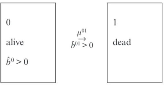
In general, one must approach the Bellman system by numerical methods. However, for the life annuity and for the term insurance which are insurances on an infinite time horizon, explicit solutions can be obtained in case of constant mortality. In a survival model as illustrated in Figure 2 a life annu-ity is a rate of benefits b0_{> 0 until death whereas a term insurance is a lump} sum benefit b01_{> 0 upon death. One nice thing about this situation is that} the system reduces to one variational equality since the optimal value func-tion after transifunc-tion to the state “dead” becomes zero. Furthermore, due to the infinite time horizon and the constant mortality we get rid of the time dependence. 0 alive b0_{> 0} 1 dead m01 → b01_{> 0}

For a life annuity the Bellman system reduces to x x xx k ( , ) ( ) ( , ) ( ) ( , ) , ( , ) ( , ). inf V x k r x V x k x ak V x k V x k V x k V pls p s _g m 0 21 1 p g 2 2 2 # $ - + - - + ^ h 6 E

In order to make the system look like the system in Hindi and Huang (1993), we change the variable u=ak, such that

x x u xx ( , ) ( ) ( , ) ( , ) , ( , ) ( , ), inf V x r x V x x V x V x V x u pls u p s _{g u} m u u b u 0 21 1 p g 2 2 2 # $ - + - - + ^ h 6 E with . a V b = The boundary condition for x= 0 is

, ( )

V 0 u e ms_g1 ak dsg _{gm u}1 g

0

=

#

3 - =

^ h

This system is equal to the system obtained in Hindi and Huang (1993). We can therefore refer directly thereto for the derivation of the optimal strategy and just quote their result with our parameters. For the derivation, Hindi and Huang (1993) make the following assumptions

> , ( ) > . r r m g _gl g b m 2 1 11 1 2 + --

-b

l

Given these assumptions the value function takes the form

( , ) , , , , V x k c k c k x d c ak x d c c ak x a ak x V g g g 1 2 3 # $ = + + -` j

*

where c1_,c2_,c3_{are constants which are determined by the model parameters,} and where

( ) ( ) , . c _rr u r r u r d _c c b l b b l b b m b g 2 2 4 1 1 2 1 2 2 1 2 2 = + + + + - ₊ + + + - + = -

-`

j

^ h

The optimal strategy is given by a constant investment in the risky asset sim-ilar to the classical solution but with greplaced by the constant cgiven above by the model parameters, i.e.

. c

p = _1-1 _sl

As for optimal dividend payments, these should keep the surplus below the boundary

. akd =_{k c}V1-_-c_g For a term insurance, the Bellman system reduces to

x x xx k ( , ) ( ) ( , ) ( ) ( , ) , ( , ) ( , ). inf V x k r r x V x k x ak V x k V x k V x k V p p s _{m g} 0 21 1 p g 2 2 2 # $ - + -- - -^ ^

b

h h

l

6 E

In order to make the system look like the system in Hindi and Huang (1993), we change the variable u₌mg1_{, such that the system can be written as above with}

. a

V

b ₌ mg1

Given this b, the optimal value function, optimal investment and optimal div-idend strategy are as in the life annuity case.

ACKNOWLEDGMENTS

The author would like to thank the referees and Peter Holm Nielsen for their comments on the first version of this paper.

REFERENCES

BJÖRK, T. (1994) Stokastisk kalkyl och kapitalmarknadsteori. Lecture notes, Royal Institute of Technology, Stockholm.

CAIRNS, A.J.G. (2000) Some notes on the dynamics and optimal control of stochastic pension

fund models in continuous time,ASTIN Bulletin30(1), 19-55.

FLEMING, W.H. and RISHEL, R.W. (1975) Deterministic and Stochastic Optimal Control, Springer-Verlag.

HANSEN, M.S. (2001) Optimal portfolio policies and the bonus option in a pension fund. Tech-nical report, Department of Finance, University of Odense.

HINDI, A. and HUANG, C. (1993) Optimal consumption and portfolio rules with durability and local substitution.Econometrica61(1), 85-121.

HOEM, J.M. (1969) Markov chain models in life insurance.Blätter der Deutschen Gesellschaft für Versicherungsmathematik9, 91-107.

JENSEN, B.A. and SØRENSEN, C. (2001) Paying for minimum interest rate guarantees: Who should

compensate who? European Financial Management7, 183-211.

KORN, R. and KRAFT, H. (2001) A stochastic control approach to portfolio problems with stochastic interest rates.SIAM Journal of Control and Optimization40(4), 250-1269.

KORN, R. and KREKELM. (2002) Optimal portfolios with fixed consumption or income streams. Technical report, Fraunhofer ITWM, Germany.

MERTON, R.C. (1969) Lifetime portfolio selection under uncertainty: The continuous time case.

Review of Economics and Statistics51, 247-257.

MERTON, R.C. (1971) Optimum consumption and portfolio rules in a continuous time model. Journal of Economic Theory3, 373-413; Erratum 6 (1973); 213-214.

NORBERG, R. (1999) A theory of bonus in life insurance.Finance and Stochastics3(4), 373-390.

RICHARD, S.F. (1975) Optimal consumption, portfolio and life insurance rules for an uncertain lived individual in a continuous time model.Journal of Financial Economics2, 187-203. STEFFENSEN, M. (2000a) Contingent claims analysis in life and pension insurance.Proceedings

AFIR 2000, 587-603.

STEFFENSEN, M. (2000b) A no arbitrage approach to Thiele’s differential equation.Insurance: Mathematics and Economics27, 201-214.

STEFFENSEN, M. (2001) On valuation and control in life and pension insurance. Ph.D.-thesis, Laboratory of Actuarial Mathematics, University of Copenhagen.

MOGENSSTEFFENSEN

Laboratory of Actuarial Mathematics Institute of Mathematical Sciences University of Copenhagen

Universitetsparken 5 DK-2100 Copenhagen Ø, Denmark