A DISCRETE-TIME MODEL OF TCP WITH ACTIVE QUEUE MANAGEMENT

A DISCRETE-TIME MODEL OF TCP WITH ACTIVE

QUEUE MANAGEMENT

by

Hui Zhang

B.Sc., Institution of Information and Communication,

Dong Hua University, P. R. China, 2001

THESIS SUBMITTED IN PARTIAL FULFILLMENT OF

THE REQUIREMENTS FOR THE DEGREE OF

Master of Applied Science

In the School

of Engineering Science

© Hui Zhang 2004

SIMON FRASER UNIVERSITY

August 2004

All rights reserved. This work may not be

reproduced in whole or in part, by photocopy

or other means, without permission of the author.

APPROVAL

Name:

Hui Zhang

Degree:

Master of Applied Science

Title of Thesis:

A Discrete-Time Model of TCP with Active Queue

Management

Examining Committee:

Chair:

Dr. Glenn H. Chapman

Professor, School of Engineering Science

_______________________________________

Dr. Ljiljana Trajkovi

ć

Senior Supervisor

Professor, School of Engineering Science

_______________________________________

Dr. Uwe Gläesser

Supervisor

Associate

Professor, School of Computing Science

_______________________________________

Dr. Qianping Gu

Examiner

Professor, School of Computing Science

ABSTRACT

The interaction between Transmission Control Protocol (TCP) and Active Queue Management (AQM) can be captured using dynamical models. The communication network is viewed as a discrete-time feedback control system, where TCP adjusts its window size based on packet loss detection during the previous Round Trip Time (RTT) interval.

In this research, a discrete-time dynamical model is proposed for the interaction between TCP and Random Early Detection (RED), one of the most widely used AQM schemes in today’s Internet. The model, constructed using an iterative map, captures the detailed dynamical behaviour of TCP/RED, including the slow start and fast retransmit phases, as well as the timeout event in TCP. Model performance for various RED parameters is evaluated using the ns-2 network simulator. The results are then compared with other existing models. Based on evaluations and comparisons of our results, we can conclude that the proposed model captures the dynamical behaviour of the TCP/RED system. In addition, the model provides reasonable predictions for system parameters such as RTT, packet sending rate, and packet drop rate. An extension of the proposed model is also presented, which is a dynamical model of TCP with Adaptive RED (ARED), a modified AQM algorithm based on RED.

ACKNOWLEDGEMENTS

I would like to thank my senior supervisor, Professor Lijljana Trajković, for her support,

guidance, and knowledge. I greatly appreciate that she gave me this precious chance to continue my studies and become a member of the Communication Networks Lab. In addition, I thank her for encouragement, great help and sincere care.

At the same time, I would like to acknowledge the supports of all of the members in our

lab, especially Judy Liu, Kenny Shao, Nikola Cackov, Vladimir Vukadinović, and Wan Zeng

Gang.

My special thanks to Dr. Qianping Gu and Dr. Uwe Glaesser for their valuable comments and for serving on my supervisory committee.

TABLE OF CONTENTS

Approval...ii

Abstract ...iii

Acknowledgements... iv

Table of Contents ... v

List of Figures ...vii

List of Tables... ix

1

Chapter One: Motivation ...

1

2

Chapter Two: Background ... 3

2.1 TCP

algorithm... 3

2.1.1

TCP congestion control ... 3

2.1.2 TCP

implementations ... 5

2.2

RED algorithm and evaluation of its parameters... 7

2.2.1

Active Queue Management ... 7

2.2.2 RED

algorithms ... 8

2.2.3

Evaluation of RED parameters ... 11

2.2.4

Recent studies on AQM... 13

2.3

Simulation tool: ns-2... 14

3

Chapter Three: A survey of existing models ...

1

5

3.1

Overview of modeling TCP Reno ... 16

3.2

Overview of modeling TCP Reno with RED ... 20

4

Chapter Four: A discrete approach for modeling TCP RENO with

Active Queue Management ... 26

4.1 TCP/RED

model ... 26

4.1.1

Case 1: No loss ... 28

4.1.2

Case 2: One packet loss ... 30

4.1.3

Case 3: At least two packet losses ... 30

4.2

Properties of the S-RED Model ... 33

4.3 Model

validation ... 34

4.3.1

Validation with default RED parameters... 35

4.3.2

Validation for various queue weights w

... 41

4.3.3

Validation for various drop probabilities p

... 45

4.3.4

Validation with various thresholds q

and q

... 49

4.3.5 Validation

summary ... 52

4.4

Comparison of S-RED model and M-model ... 53

4.4.2

Comparison for various queue weights w

... 54

4.4.3

Comparison for various drop probabilities p

... 57

4.4.4

Comparison for various thresholds q

and q

... 58

4.5 Model

modification... 60

4.6

Model extension: TCP with Adaptive RED (S-ARED model) ... 64

4.6.1

S-ARED model validation... 67

4.6.2 Model

evaluation ... 70

5

Chapter Five: Conclusions and future work ... 72

LIST OF FIGURES

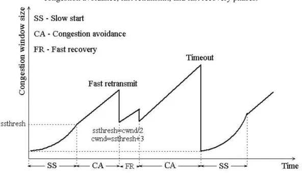
Figure 1. Evolution of the window size in TCP Reno, consisting of slow start,

congestion avoidance, fast retransmit, and fast recovery phases. ... 4

Figure 2. RED drop probability as a function of the average queue size... 10

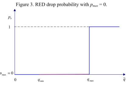
Figure 3. RED drop probability with p

= 0... 12

Figure 4. RED drop probability with p

= 1... 12

Figure 5. TCP window size evolution... 16

Figure 6. Topology of the modeled and simulated network. ... 27

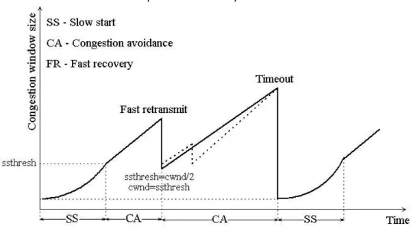
Figure 7. Evolution of the window size in the S-RED model. The fast recovery

phase has been simplified... 34

Figure 8. Topology of the simulated network. ... 35

Figure 9. Evolution of the window size with default RED parameters: (a) S-RED

model, and (b) zoom-in, (c) ns-2 simulation results and (d) zoom-in.

Waveforms show good match between the S-RED model and the ns-2

simulation results... 36

Figure 10. Evolution of the average queue size with default RED parameters: (a)

S-RED model and (b) in, (c) ns-2 simulation result and (d)

zoom-in. The average queue size obtained using the S-RED model is higher

than the average queue size obtained using ns-2 simulations. ... 38

Figure 11. S-RED model: evolution of the window size for w

= 0.006... 41

Figure 12. ns-2: evolution of the window size for w

=0.006. ... 42

Figure 13. Comparison of the average queue size for various w

... 43

Figure 14. S-RED model: evolution of the window size for p

= 0.5... 46

Figure 15. ns-2: evolution of the window size for p

= 0.5... 46

Figure 16. Comparison of the average queue size for various p

... 47

Figure 17. S-RED model: evolution of the window size for q

= 10 packets. ... 49

Figure 18. ns-2: evolution of the window size for q

= 10 packets. ... 50

Figure 19. Comparison of the average queue size for various q

and q

... 50

Figure 20. M-model: evolution of the average queue size with default RED

parameters. ... 54

Figure 22. Comparison of the average queue size for various p

... 57

Figure 23. Comparison of the average queue size for various q

and q

... 59

Figure 24. S-RED model with modification: (a) evolution of the window size and

(b) the average queue size. ... 61

Figure 25. Comparison of the average queue size for various w

... 62

Figure 26. Comparison of the average queue size for various p

... 63

Figure 27. Comparison of average queue size for various q

and q

... 63

Figure 28. Evolution of the window size: (a) S-ARED and (b) ns-2 simulation

results... 68

Figure 29. Evolution of the average queue size: (a) S-ARED and (b) ns-2

simulation results... 69

LIST OF TABLES

Table 1. Default RED parameters in ns-2. ... 35

Table 2. Statistic values of state variables for S-RED model and ns-2... 40

Table 3. Statistical analysis of window size for various w

... 43

Table 4. Statistical analysis of the average queue size for various w

... 44

Table 5. System variable for various w

... 45

Table 6. Statistical analysis of the window size for various p

... 47

Table 7. Statistic analysis of the average queue size for various p

... 48

Table 8. System parameters for various p

... 48

Table 9. Statistical analysis of the window size for various q

and q

... 51

Table 10. Statistical analysis of the average queue size for various q

and q

.

... 51

Table 11. Statistic analysis of the average queue size for various w

. ... 52

Table 12. System parameters. ... 53

Table 13. System variables for various w

. ... 56

Table 14. System variables for various p

... 58

Table 15. System parameters with various q

and q

.

... 60

Table 16. Default ARED parameters in ns-2. ... 67

Table 17. Average values of the window size, average queue size, and system

parameters. ... 70

1

CHAPTER ONE: MOTIVATION

Today’s Internet applications, such as the World Wide Web, file transfer, Usenet news, and remote login, are delivered via the Transmission Control Protocol (TCP). With an increasing number and variety of Internet applications, congestion control becomes a key issue. Active Queue Management (AQM) interacts with TCP congestion control mechanisms, and plays an important role in meeting today’s increasing demand for quality of service (QoS). Random Early Detection (RED), a widely employed AQM algorithm, is a gateway-based congestion control mechanism. An accurate model of TCP with RED can aid in the understanding and prediction of the dynamical behaviour of the network. In addition, the model may help in analyzing the system’s stability margins, and providing the design guidelines for selecting network parameters. These design guidelines are important for network designers whose aim is to improve network robustness. Therefore, modeling TCP with RED is an important step towards improving the network efficiency and the service provided to Internet users.

Modeling TCP performance has received increasing attention during the last few years due to the benefits it offers to the networking community. Analytical TCP models enable researchers to closely examine the existing congestion control algorithms, address their shortcomings, and propose methods for their improvement. They may also be used to compare various TCP schemes and implementations, and to determine their performance under various operating conditions. Moreover, these models help examine the interactions between TCP and the queuing algorithms implemented in routers. Hence, they aid in the improvement of existing algorithms and in designing better algorithms, such as AQM techniques. Finally, such models offer the possibility of defining TCP-friendly behaviour in terms of throughput for non-TCP flows that coexist with TCP connections in the same network.

In this thesis, our goal is to model TCP and to investigate the nonlinear phenomena in a TCP/RED system. We are particular interested in the bifurcation and chaos phenomena that are recently observed in a TCP/IP network [24]. We use an iterative map to model the system. A second-order discrete model is derived in order to capture the interactions of the TCP congestion control algorithm with the RED queuing mechanism. We use the concepts proposed in [34] and construct a nonlinear dynamical model of TCP/RED that employs two state variables: the window size and the average queue size. The change of the window size reflects the dynamics of TCP congestion control, while the average queue size captures the queue dynamics in the RED gateway. The novelty of the proposed model is in capturing the detailed dynamical behaviour of

TCP/RED. The proposed model, called S-RED model, considers the slow start, the congestion

avoidance, the fast retransmit, and parts of fast recovery phases. It also takes into account timeout events. In addition, the interaction of TCP with Adaptive RED (ARED), a revised RED algorithm,

is discussed. We also derive a discrete-time model for TCP with ARED, named S-ARED model,

2

CHAPTER TWO: BACKGROUND

2.

1

TCP algorithm

TCP, or Transmission Control Protocol, is designed to provide a connection-oriented, reliable, and byte-stream service [42]. Before communication can begin between two hosts, a connection must be established by employing a three-way handshake algorithm. This algorithm also allows the sender and receiver to initialize and synchronize important parameters, sequence numbers, advertised window size, and maximum segment size. The basic concept of the TCP congestion control algorithm is window based flow control. The window size determines the amount of data to be sent by the source. Its value will increase when all of the acknowledgements are properly received; otherwise, the window size may decrease. There are numerous versions of TCP implementations. In this research, the primary focus is on TCP Reno [1], [20], [21], as it is one of the most widely used versions in today’s network. Other versions of TCP implementations are briefly overviewed in Section 2.1.2

2.

1

.

1

TCP congestion control

To adjust the window size, the TCP Reno congestion control mechanism employs four algorithms: slow start, congestion avoidance, fast retransmit, and fast recovery, as shown in Figure 1. They were introduced by Jacobson [20], [21] and are described in RFCs 1122 [4] and 2581 [1].

Figure 1. Evolution of the window size in TCP Reno, consisting of slow start, congestion avoidance, fast retransmit, and fast recovery phases.

In order to avoid congesting the network with large data bursts, an established TCP connection first employs the slow start algorithm to detect the available bandwidth in the network.

Typically, a TCP sender initializes its congestion window (cwnd) to one or two segments,

depending on the TCP implementation. Upon receipt of each acknowledgement (ACK) for new

data, TCP increments cwnd by one segment size. When cwnd exceeds a threshold (ssthresh), the

sender switches from slow start to the congestion avoidance phase. During congestion avoidance,

cwnd is incremented by one segment size per Round Trip Time (RTT). Each time a packet is sent

by the sender, a timer is set. Packet loss is detected by this timeout mechanism if the timer expires before receipt of the packet has been acknowledged. When multiple packets are dropped from the same window or the TCP sender does not receive enough packets to trigger fast retransmit, the TCP sender may need to wait for a timeout to occur before the lost packets get retransmitted. If a

packet loss is detected by the timeout mechanism, the TCP sender adjusts its ssthresh and

switches back to slow start. The duration of the timeout (TO) is usually updated with the RTT. If another timeout occurrs before the lost packet is successfully retransmitted, the period of timeout (TO) doubles to twice the value of the previous duration (2TO). This duration time continues to

increase exponentially for each unsuccessful retransmission until the timeout period reaches 64 times the first timeout period (64TO). The timeout period then remains constant at 64TO.

The fast retransmit algorithm is used for recovery from losses detected by triple duplicate ACKs; i.e. four consecutive ACKs acknowledging the same packet. When an out-of-order segment is received by a TCP receiver, a duplicate ACK is immediately sent out to inform the sender of the sequence number for the packet that the receiver is expecting. The receipt of triple duplicate ACKs is used as an indication of packet loss. The TCP sender reacts to the packet loss

by reducing cwnd by half and by re-transmitting the lost packet without waiting for the

retransmission timer to expire.

The fast recovery algorithm is used to control data transmission after fast retransmission

of the lost packet. During this phase, the TCP sender first sets its ssthresh to half of the current

cwnd. Then it increases its cwnd for each duplicate ACK received. The fast recovery algorithm

recognizes each duplicate ACK as an indication that one packet has left the channel and has reached the destination. Since the number of outstanding packets has decreased by one, the TCP

sender is allowed to increment its cwnd. When a non-duplicate ACK is received, TCP sender sets

cwnd equal to ssthresh and switches from fast recovery to the congestion avoidance phase.

2.

1

.2

TCP implementations

Older TCP implementations, released in the early 1980s, employed a simple window-based congestion control mechanism as specified in RFC 793 [38].

TCP Tahoe, released in the late 1980s, employed the slow start, congestion avoidance, and fast retransmit algorithms. When packet loss is detected, the sender retransmits the lost packet, reduces the congestion window to one and enters slow start. When the sender receives an ACK for the retransmitted packet, it will continue to send packets from the sequence number indicated in the ACK even if some of them are already sent. Thus, if any packet is lost in the

meantime, it will be automatically retransmitted via this go-back procedure. In other words, TCP Tahoe will not have to wait for a timeout in the case where multiple packets are lost from the same window. However, frequent losses will force the TCP sender to operate in slow start phase for most of the time.

TCP Reno, introduced in the early 1990s, added the fast recovery algorithm. This algorithm does not require slow start for every packet loss. Once the three duplicate ACKs are received, the TCP sender retransmits the lost packet, reduces its congestion window by half, and enters the fast recovery phase instead of the slow start algorithm. When the first non-duplicate ACK is received, the sender exits fast recovery mode and enters the congestion avoidance phase. TCP Reno's fast recovery algorithm is optimized for the case when one packet is lost from a window. When multiple packets are lost from the same window, TCP Reno generally must wait for timeout.

TCP Reno’s congestion control algorithm works well when dealing with congestion-induced loss. However it results in reduced throughput without providing any benefits. It is also inappropriate when faced with loss due to corruption rather than congestion, such as satellite networks. In addition, using ns-2 simulations, Fall and Floyd [11] demonstrated that TCP Reno exhibits poor performance in terms of link utilization whenever multiple packets are dropped from a single window of data. To alleviate this problem, they introduced two modifications to TCP Reno: TCP New-Reno and TCP SACK [25]. A large number of Internet Web servers still use TCP Reno and its variants [35]. For example, in the TCP SACK implementation, TCP receivers can inform senders exactly which segments have arrived, rather than replying on TCP’s cumulative acknowledgements. This allows a TCP sender to efficiently recover from multiple lost segments without reverting to using a costly retransmission timeout to determine which segments need to be retransmitted. It also hastens recovery and prevents the sender from becoming window limited, thus allowing the pipe to drain while waiting to learn about lost segments. This ability is

of particular benefit in keeping the pipe full and allowing transmission to continue while recovering from losses.

Other TCP implementations, such as TCP Vegas [5] and TCP Westwood [7], use various techniques to avoid congestion. They adjust the congestion window size based on estimates of the throughput at the bottleneck. For instance, TCP Vegas controls the congestion window size by estimating the RTT and by calculating the difference between the expected flow rate and the actual flow rate. It linearly adjusts TCP’s congestion window size upwards or downwards, so as to consume a constant amount of buffer space in the network. It detects packet losses earlier than Reno and uses a slower multiple decrease than Reno. TCP Vegas eliminates the need to tune the receive window to serve as an upper bound on the size of the congestion window. It can avoid network congestion without overdriving the link to find the upper bound, even when operating with large windows. TCP Vegas increases its congestion window size more slowly than Reno by measuring the achieved throughput gain after each increase to detect the available capacity without incurring loss.

2.2

RED algorithm and evaluation of its parameters

2.2.

1

Active Queue Management

A traditional DropTail queue management mechanism drops the packets that arrive when the buffer is full. However, this method has two drawbacks. First, it may allow a few connections to monopolize the queue space so that other flows are starved. Second, DropTail allows queues to be full for a long period of time. During that period, incoming packets are dropped in bursts. This causes a severe reduction in throughput of the TCP flows. One solution, recommended in RFC 2309 [2], is to employ active queue management (AQM) algorithms. The purpose of AQM is to react to incipient congestion before the buffer overflows. AQM allows responsive flows, such as

TCP flows, to react timely and reduce their sending rates in order to prevent congestion and severe packet losses.

2.2.2

RED algorithms

The most popular AQM algorithm is Random Early Detection (RED), proposed by Floyd and Jacobson [16]. The RED mechanism contains two key algorithms. One is used to calculate the exponentially weighted moving average of the queue size, so as to determine the burstiness that is allowed in the gateway queue and to detect possible congestion. The second algorithm is for computing the drop or marking probability, which determines how frequently the gateway drops or marks arrival packets. This algorithm can avoid global synchronization by dropping or marking packets at fairly evenly-spaced intervals. Furthermore, sufficiently dropping or marking packets, this algorithm can maintain a reasonable bound of the average delay, if the average queue length

is under control. The RED algorithm is given in Algorithm 1, where

q

and q is the instantaneous queue size.

Let wq be the weight factor and qk+1 be the new instantaneous queue size. At every packet

arrival, the RED gateway updates the average queue size as

1

1 (1 ) +

+ = − q ⋅ k + q⋅ k

k w q w q

q . (1)

During the period when the RED gateway queue is empty, the system will estimate the number of

packets m that might have been transmitted by the router. Hence, the average queue size is

updated as k m q k

w

q

q

=

(

1

−

)

⋅

time

on

transmissi

time

idle

m

=

_

_

where idle_time is the period that the queue is empty and transmission_time is the typical time

Algorithm 1:The pseudo-code of RED algorithm. Initialization:

q

q

q

q

q

q

q

Pb = pmax × (

q

Drop arriving packet with Pa; (if arrival packet is dropped, count = 0)

}

else if ((

q

q

Drop arriving packet; count = 0; }

The average queue size is compared to two parameters: the minimum queue threshold

qmin, and the maximum queue threshold qmax. If the average queue size is smaller than qmin, the

packet is admitted to the queue. If it exceeds qmax, the packet is marked or dropped. If the average

queue size is between qmin and qmax, the packet is dropped with a drop probability pb that is a

function of the average queue size

















⋅

−

−

≥

≤

=

otherwise

p

q

q

q

q

q

q

if

q

q

if

p

1

0

where pmax is the maximum packet drop probability. The relationship between the drop probability

and average queue size is shown in Figure 2.

Figure 2. RED drop probability as a function of the average queue size.

q max q min q max p 0 1 b p

The final drop probability pa is given by Eq. (5). It is introduced in order to avoid the severe

increase of the drop rate shown in Figure 2.

b b a

p

count

p

p

⋅

−

=

1

Here, count is the cumulative number of the packets that are not marked or dropped since the last marked or dropped packet. It is increased by one if the incoming packet is not marked or dropped.

Therefore, as count increases, the drop probability increases. However, if the incoming packet is

marked or dropped, count is reset to 0.

2.2.3

Evaluation of RED parameters

Unlike DropTail, the performance of the RED algorithm is not determined only by the

buffer size. Other parameters, such as queue weight (wq), maximum drop rate (pmax), and the two

queue thresholds (qmin and qmax), are also of great importance. The network designer should select

these appropriately, so that the system can achieve better performance.

wq is an exponentially weighted average factor, which determines the time constant for

the averaging of the queue size. If wq is too low, then the estimated average queue size is probably

responding too slowly to transient congestion. If wq is too high, then the estimated average queue

size will track the instantaneous queue size too closely, and may result in an unstable system. In

[17], quantitative guidelines are given for setting wq in terms of the transient burst size that the

queue can accommodate without dropping any packets. The optimal setting for wq is between

0.001 and 0.005.

The packet drop probability is calculated as a linear function of the average queue size if

the average queue size is between qmin and qmax. However, the maximum drop probability

determines the oscillation of the drop rate. If pmax is set too small, then the network behaves

similar to the DropTail shown in Figure 3. However, if this value is set too high (Figure 4), the packet drop probability increases, thus enforcing the system to oscillate severely and experience a decrease in throughput. It has been shown that steady-state packet drop rates of 5% to 10% would

not be unusual at a router. There is, therefore, no need to set pmax higher than 0.1 for real network

Figure 3. RED drop probability with pmax = 0. q max q min q b p 0 0 max = p 1

Figure 4. RED drop probability with pmax = 1.

q max q min q 1 max= p b p 0 0

The optimal values for qmin and qmax depend on the desired average queue size. If the

typical traffic patterns are fairly bursty, then qmin must be correspondingly large to allow the link

utilization to be maintained at an acceptably high level. This value should also be associated with

the buffer size of the network. If qmin is set too small, it leads to low bandwidth utilization.

Conversely, if qmin is set too high, it may result in unfair competition for bandwidth among

multiple links, thereby cancelling out the benefits of the RED algorithm. The optimal value for

gateway functions most effectively when the difference between qmax and qmin is larger than the typical increase in the calculated average queue size, in one roundtrip time [16]. A useful rule of

thumb is to set qmax to at least twice the size of qmin. If the difference between qmax and qmin is set

too small, then the computed average queue size can regularly oscillate up to qmax. This behaviour

is similar to the oscillations of the queue size up to the maximum queue size experienced with DropTail gateways.

2.2.4

Recent studies on AQM

Although RED is one of the most prominent active queue management schemes, a number of research efforts have focused on possible shortcomings of the original RED algorithm and have proposed modifications and alternatives, such as Adaptive RED (ARED) [15], CHOKe [36], BLUE [13], Stabilized RED, Flow RED, and Balanced RED. For example, ARED, proposed in 2001, aims to improve the robustness of the original RED with only minimal changes. It attempts to achieve a stable average queue size around a pre-set target value. Its default setting is

half way between qmin and qmax. It has been shown [15] through various simulation results that

ARED tends to be more stable and performs better than the original RED. The key modification of ARED is updating the maximum drop rate for every interval period so that the packet drop probability changes more slowly than in the original RED algorithm. The calculation of the

modified pmax is given in Algorithm 2.

Other algorithms are aimed at solving problems that the original RED could not address. For instance, CHOKe [36] is designed to achieve better performance on fairness, while the BLUE algorithm performs queue management directly based on packet loss and link utilization, rather than on the instantaneous or average queue lengths. In addition, the BLUE algorithm can react faster to substantial increases of traffic load than the RED algorithm.

Algorithm 2: The pseudo-code of ARED algorithm.

For every interval (usually the interval is set to 0.5 seconds): {

If ((

q

pmax = pmax +

α

Else if ((

q

pmax = pmax *

β

} where

target: [qmin + 0.4 * (qmax – qmin), qmin + 0.6 * (qmax – qmin)];

:

α

:

β

2.3

Simulation tool: ns-2

Ns-2 [33] is a discrete event network simulator targeted at networking research, which is currently supported by the Defence Advanced Research Project Agency (DARPA) and the National Science Foundation (NSF). It provides substantial support for simulation of TCP, routing, and multicast protocols over wired and wireless (local and satellite) networks. In this research, ns-2 was used to perform the network simulation and the simulation results were used to evaluate the proposed S-RED model.

3

CHAPTER THREE: A SURVEY OF EXISTING MODELS

Many papers have been published on different models for TCP. In this chapter, we describe the different models and implementations of TCP.

From the viewpoint of flow characteristics, analytical TCP models can be classified in three categories based on the duration of the TCP flows. This, in turn, determines the TCP congestion control algorithms to be modeled and the aspects of TCP performance that can be captured by the model [22]. The first category models short-lived flows where TCP performance is strongly affected by the connection establishment and slow start phases [30]. These models typically approximate average latency or completion time, i.e., the time it takes to transfer a certain amount of data. The second category models long-lived flows, which characterize the steady-state performance of bulk TCP transfers during the congestion avoidance phase [28], [32], [34], [41]. These models approximate aspects such as the window size, average throughput, sending rate, and goodput (goodput is used to describe the data that has been properly received). The final category includes models for flows of arbitrary duration, i.e., those that can accommodate both short and long-lived flows [6], [8]. All these models provide functions to compute the average values of throughput, sending rate, goodput, or latency of TCP flows.

From the control theoretic point of view, the developed models of TCP and TCP/RED [18], [19], [23], [24], [31], [39], [40], can be classified into two types: averaged models and iterative map models. An averaged model is described by a set of continuous differential

equations. It neglects the detailed dynamics and only captures the low frequency characteristicsof

the system. It can be used to analyze the steady-state performance and to predict low frequency slow-scale bifurcation behaviour, such as Hopf bifurcations. Examples of such models are given in [18], [19], [23]. In contrast, an iterative map model has a discrete-time form and employs a set

of difference equations. It provides relatively complete dynamical information. The discrete-time map is adequate to explore nonlinear phenomena such as period-doubling and saddle-node bifurcations, which may appear across a wide spectrum of frequencies and cause the existence of solutions in the high frequency range. Examples of iterative maps are given in [24], [39], [40].

3.

1

Overview of modeling TCP Reno

Several models have been proposed in order to analyze the performance of packet networks. Prior to 1997, research was primarily focused on modeling the TCP congestion avoidance phase and ignored slow start, fast recovery, and timeout events. In [27], the authors

assume random packet loss with a constant probability p, which means that approximately 1 / p

packets are to be sent followed by one packet loss. Hence, the evolution of the cwnd results a

periodic sawtooth shown in Figure 5.

The cwnd is halved when a packet is dropped. During this period, there are

8

3

2

)

2

(

2

1

W

W

W

W

+

⋅

=

⋅

8

3

1

W

p

=

As cwnd increases by one packet size every RTT, the time required to send

8

3

W

packets is

RTT W _⋅

2 . Hence, the sending rate becomes

p

RTT

C

M

W

RTT

W

M

BW

⋅

⋅

=

⋅

⋅

=

2

8

3

3

/

2

By selecting an appropriate value for the constant C, the model is able to estimate the TCP performance over a range of loss conditions and in environments with both DropTail and RED queuing [28]. However, the prediction of the model is not very accurate, because it simplifies the TCP congestion control algorithm.

A more precise steady-state model of TCP Reno, introduced in [34], also employs the steady-state sending rate as a function of loss rate and RTT of a bulk data transfer TCP flow. The model provides a detailed explanation of the TCP algorithm. In addition to capturing the essence of TCP’s fast retransmit and congestion avoidance phases, it also accounts for the effect of the

timeout mechanism, which is important from a modeling perspective. The model also takes into account delayed ACKs, which are not discussed in this research. However, this model ignores the influence of queue management schemes.

In [34], authors take several steps to analyze the sending rate by separating the congestions caused by three-duplicate ACKs and timeouts. They also consider other upper bound parameters, such as advertised window size. The model describes the system in terms of duration

of the RTT, called rounds. The model is built based on the following assumptions: RTT is a

constant and it is considered to be independent of the window size; the maximum window size is also constant; only long lived connections are studied, which implies that the source buffer always has enough data to send; any packet loss is considered as link congestion; the packet loss is correlated within one round, i.e., if a packet is lost, then the remaining packets transmitted in that round are also lost. However, the packet loss is independent in different rounds. Slow start and fast recovery phases are not considered in this model. The following two situations describe the cases studied in [34].

Case one: The timeout is not considered and congestion is only detected by three duplicate ACKs.

The expectation of the total number of packets Y that are to be transmitted before a

packet loss, is given by

p

p

p

W

E

p

p

Y

E

3

5

8

1

]

[

1

]

[

−

+

=

+

−

=

where p is the drop probability and W is the value of congestion window size. The time required

) 3 5 8 3 ( 2 ] [ p p RTT A E = + − . (9)

From Eqs (8) and (9), the sending rate BW can be derived as

)

3

5

8

3

(

2

3

5

8

1

]

[

]

[

p

p

RTT

p

p

p

A

E

Y

E

BW

−

+

−

+

=

=

Equation (10) can be simplified to Eq. (11) for small values of p as

p RTT BW 2 3 1 = . (11)

Case Two: The loss indication is detected by three duplicate ACKs and timeouts: The sending rate in Eq. (10) is modified to

] [ ] [ ] [ ] [ TO Z E Q A E R E Q Y E BW ⋅ + ⋅ + = , (12)

where Q is the probability that a packet loss is detected by a timeout, R is the total number of

packets that are to be sent during the timeout interval, and ZTO _{is the duration of the timeout. The}

final simplified equation (for small values of p) for the sending rate is

) 32 1 ( ) 8 3 3 , 1 min( 3 2 1 2 0 p p p T p RTT BW + + ≈ , (13)

where T0 is the initial value of a timeout.

The model developed in [6] is a further extension of the model developed in [34], which aims for a more precise model of TCP latency. The model takes into account the time used to set up the connection, which is known as the three-way handshake algorithm, and the slow start phase. This information is very important for modeling short-lived connections. In addition, the model considers detailed information about data transmission including congestion avoidance, fast retransmit, fast recovery, and timeout evens. The total latency of the network is

]

[

]

[

]

[

]

[

]

[

T

E

T

E

T

E

T

E

T

E

=

+

+

+

where Tss is the duration of data transfer within the slow start and congestion avoidance phases,

Tloss is the cost for timeout or fast recovery, Tca is the time required to transmit the remaining

packets before loss recovery, and Tdelack is the cost of the delayed ACKs.

3.2

Overview of modeling TCP Reno with RED

A simplified first-order discrete nonlinear dynamical model was developed for simplified TCP with RED control in [24], [39], [40]. The exponentially weighted average queue size was used as the state variable. The model describes the system dynamics over large parameter variations and samples the buffer occupancy at certain time instances. This dynamical model was used to investigate the stability, bifurcation, and routes to chaos of a network for various system parameters. Based on the developed model, the authors demonstrated that nonlinear phenomena, such as bifurcation and chaos, might occur if the system parameters were not properly selected. However, this discrete model neglects the dynamics of TCP. The derived map is given by

        ⋅ − ⋅ ⋅ + ⋅ − ≤ ⋅ + ⋅ − ≥ ⋅ − = + otherwise M d C p K N w q w q q if B w q w q q if q w q k ave k ave l ave k ave k ave u ave k ave k ave k ) ( ) 1 ( ) 1 ( ) 1 ( 1 , (15)

where q_kave₊₁: average queue size in round k+1

ave

k

q : average queue size in round k

q_uave: upper bound of the average queue size

ave l

q : lower bound of the average queue size

w

B: buffer size

N: number of TCP connections

K: constant [1,

8

/

3

p

C: link capacity

d: round-trip propagation delay

M : packet size.

In [31], a second-order nonlinear dynamical model was developed to examine the interactions of a set of TCP flows with RED. The model employs the fluid-flow and stochastic differential equations. Window size and average queue length are used as state variables. From a set of coupled ordinary differential equations, the authors develop a numerical algorithm to obtain the transient average behaviour of queue length, round trip time, and throughput of TCP flows. This model is described by nonlinear differential equations that employ the average values of key network variables, given by

C t W t R t N t q t R t p t R t R t R t W t W t R t W − ⋅ = − ⋅ − − ⋅ − = ) ( ) ( ) ( ) ( )) ( ( )) ( ( 2 )) ( ( ) ( ) ( 1 ) ( D D , (16)

whereW(t): expected TCP window size

q(t): expected queue length

R(t): round trip time

N(t): load factor (number of TCP sessions)

p(t): probability of packet mark/drop

C: link capacity.

A third-order dynamical model that describes the interaction of TCP flows with an RED controlled queue was developed in [23]. The state variables of the model are average queue length, instantaneous queue length, and throughput. The TCP sources are idealized to operate only during the congestion avoidance phase, when the congestion window size follows the rule of linear increase and multiplicative decrease. This dynamical model is used to explore various parameter settings and observe transient and equilibrium behaviour of the system. The validity of the model is verified by comparison with simulation results. The interaction between TCP and RED is modeled as

))

(

(

))

(

(

))

(

(

))

(

(

)

(

)

(

)

(

))

2

/

(

1

(

)

(

)

(

2

)

2

/

(

)

(

)))

(

(

1

(

)))

(

(

1

(

)))

(

(

1

(

)

2

/

(

)

(

))

(

)

(

(

)

2

/

(

)

(

t

q

t

s

p

t

q

t

s

p

t

P

t

R

t

R

m

R

t

P

R

t

t

m

R

t

P

t

dt

d

t

q

t

s

p

t

q

R

t

t

q

ct

d

t

s

t

q

R

t

t

s

dt

d

π

π

λ

λ

λ

λ

λ

π

µ

π

λ

β

λ

⋅

−

+

=

−

⋅

−

−

+

−

⋅

⋅

−

−

=

−

−

−

⋅

−

⋅

−

=

−

⋅

−

=

where s(t): expectation of the exponentially averaged queue length

q(t): expectation of the instantaneous queue length

λ

(t

)

P

(t

)

π

(

q

(

t

))

π

(

q

(

t

))

p: drop probability

R: round trip time

β

m

In [18], [19], the authors describe a second-order linear model for TCP and RED, by linearizing the fluid-based nonlinear TCP model. Window size and average queue length are used as state variables of the system. The authors performed analysis of TCP interactions with RED from a control theoretic viewpoint. They presented design guidelines for choosing RED parameters that led to local stability of the system. In addition, they proposed two alternative controllers to improve the transient behaviour and stability of the system: a proportional (P) controller that possesses a good transient response, but suffers from steady-state errors in queue regulation, and a classical proportional-integral (PI) controller that exhibits zero steady-state regulation error and acceptable transient behaviour. One important contribution of this work is providing a good example of how to use classical control theory to solve problems in complex communication systems. The linearized model around the operating point is described as

) ( 1 ) ( ) ( ) ( 2 )) ( ) ( ( 1 )) ( ) ( ( ) ( 0 0 2 2 0 0 2 0 0 2 0 t q R t W R N t q C t p N C R R t q t q C R R t W t W C R N t W δ δ δ δ δ δ δ δ δ − = − ⋅ − − − ⋅ − − + ⋅ − = , (18) where

δ

W

=

W

−

W

q

q

q

=

−

δ

p

p

p

=

−

δ

(

W

,

q

,

p

)

W: expectation of the TCP window size

q: expectation of the queue length

R

C: link capacity

T_p: propagation delay

N: load factor (number of TCP sessions)

p: probability of packet mark/drop.

A multi-link multi-source model, developed in [27], was used to study the stability of a general TCP/AQM system. A local stability condition in the case of a single link with heterogeneous sources and the stability region of TCP/RED were derived. The state variables of this model are window size, instantaneous queue length, and average queue length. The authors demonstrated that TCP/RED becomes unstable when the link capacity increases. Finally, they devised a new distributed congestion control algorithm that maintains local stability for arbitrary

delay, capacity, and traffic load. Preliminary simulation results were provided in order to illustrate the model’s behaviour.

4

CHAPTER FOUR: A DISCRETE APPROACH FOR

MODELING TCP RENO WITH ACTIVE QUEUE

MANAGEMENT

4.

1

TCP/RED model

The basic idea behind RED is to sense impending congestion before it happens and to try to provide feedback to senders by either dropping or marking packets. Hence, from the control theoretic point of view, the network may be considered as a complex feedback control system. TCP adjusts its sending rate depending on whether or not it has detected a packet drop in the previous RTT interval. The drop probability of RED can be considered as the control law of the network system. Its discontinuity is the main reason for oscillations and chaos in the system. Hence, it is natural to model the network system as a discrete model. In this thesis, we model the

TCP/RED system using a stroboscopic map, which is the most widely used type of discrete-time

maps for modeling power converters [3], [9], [10], [43]. This map is obtained by periodically sampling the system state. In our study, the sampling period is one RTT. Since window size and queue size behave as step functions of RTT, one RTT is the sampling period that captures their changes [14]. Higher sampling rates would not significantly improve the accuracy of the model. Conversely, lower sampling rates would ignore the changes and affect the model accuracy.

The state variables employed in the S-RED model are window size and average queue size. These state variables capture the detailed behaviour of TCP/RED. Variations of the window size reflect the dynamics of TCP congestion control. The window size increases exponentially and linearly during the slow start and the congestion avoidance phases, respectively. It multiplicatively decreases when loss occurs. The average queue size captures the queue dynamics

in RED as it is updated upon every packet arrival. In our study, we did not consider instantaneous queue size as an independent state variable.

The S-RED model is suited for investigating the nonlinear behavior of TCP/RED and analyzing the system’s transitions into chaos. Hence, in this thesis, we consider a simple network topology as shown in Figure 6. It consists of one TCP source, two routers, and a destination. RED is employed in the first router. A TCP Reno connection is established between the source and the destination. Data packets are sent from the source to the destination, while traffic in the opposite direction consists of ACK packets only.

We made several assumptions in order to construct an approximate model. We assume that ACK packets are never lost. The connection is long-lived and the source always has sufficient

data to send. Round trip propagation delay d between the source and destination is constant. Data

packet size M is constant. The link that connects the two routers is the only bottleneck in the

network. We also assume that the timeout is only caused by packet loss and that the duration of the timeout period is 5 RTTs [14]. The state variables of the system are sampled at the end of every RTT period. We assume that the queue size is constant during each sampling period. The model includes three cases, depending on the number of packets lost in the previous RTT period: no loss, single loss, and multiple packet losses.

Figure 6. Topology of the modeled and simulated network.

Source Router 1 Router 2 Destination

4.

1

.

1

Case

1

: No loss

Let Wk, qk, and

q

respectively, at the end of the sampling period k. If no packet is dropped during the last RTT

period, TCP Reno increases its window size. The window size is increased exponentially in the slow start phase and linearly in the congestion avoidance phase:

1 min(2 , ) min( 1, ) k k k k k W ssthresh if W ssthresh W W rwnd if W ssthresh + < = + ≥







where rwnd is the receiver’s advertised window size; i.e., the largest window size that the receiver

can accept in one round. Usually, rwnd is greater than the window size. In this case, rwnd does

not affect the variations of the window size. In the event that the window size increases linearly

and reaches the value rwnd, the window size is kept at rwnd until a loss occurs in the network.

The round trip time in k+1 round is calculated by

C M q d RTT k k ⋅ + = +1 , (20)

where

RTT

d: round trip propagation delay

C: link capacity

M: packet size.

In order to calculate the average queue size given by Eq. (1), we need to know the queue

size at the sampling period k+1. The instantaneous queue size depends on the queue size in the

previous period, the current window size, and the number of packets that have left the queue during the previous sampling period. Therefore, the instantaneous queue size is given by

M

d

C

W

C

M

q

d

M

C

W

q

M

RTT

C

W

q

q

⋅

−

=

⋅

+

⋅

−

+

=

⋅

−

+

=

)

(

where

q

k

q

1 +

k

W

Substituting qk+1 in Eq. (1) yields the average queue size:

) 0 , max( ) 1 ( ₁ 1 M d C W w q w q_k+ = − _q ⋅ _k + _q ⋅ _k+ − ⋅ . (22)

Because RED updates the average queue size at every packet arrival, q is updated Wk+1

times during the current sampling period. For the first packet arrival, the average queue size is updated according to ) 0 , max( ) 1 ( M d C W w q w q = − _q ⋅ + _q⋅ − ⋅ . (23)

For the second packet arrival, the average queue size is given by

[

]

Since we assume that queue size is constant during each period, and that there are Wk+1packet

arrivals during this time interval, q is updated Wk+1times:

) 0 , max( ) ) 1 ( 1 ( ) 1 ( ₁ 1 1 1 _M d C W w q w q W _k q k W q k k k ⋅ − ⋅ − − + ⋅ − = ₊ + + + . (25)

In summary, if p W_k⋅ _k <0.5, which implies that no packet loss occurred in the previous sampling period, the state variables of the model are

) 0 , max( ) ) 1 ( 1 ( ) 1 ( ) , 1 min( ) , 2 min( 1 1 1 1 1 M d C W w q w q ssthresh W if rwnd W ssthresh W if ssthresh W W k W q k W q k k k k k k k k ⋅ + − − ⋅ − ⋅ − =    ≥ + < = + + + + + . (26)

4.

1

.2

Case 2: One packet loss

If 0.5≤ p W_k⋅ _k <1.5, which implies that one packet loss occurred in the previous RTT

period, the congestion control mechanism of TCP Reno halves the window size in the current sampling period:

₁ 1

2

k k

W₊ = W . (27)

The average queue size is updated in the same manner as in Case 1:

) 0 , max( ) ) 1 ( 1 ( ) 1 ( 2 1 1 1 1 1 1 M d C W w q w q W W k W q k W q k k k k k ⋅ + − − ⋅ − ⋅ − = = + + + + + . (28)

4.

1

.3

Case 3: At least two packet losses

In this case p W_k⋅ _k ≥1.5, which implies that at least two packets are lost in the previous

RTT period. When multiple packets are lost from the same window, TCP Reno may not be able to send a sufficient number of new packets in order to receive three duplicate ACKs for each lost packet. The TCP source will probably have to wait for a timeout to occur before retransmitting the lost packet [11]. During the timeout period, the source does not send packets into the network. In our model, window size is equivalent to the number of packets that are sent by the source during one RTT period. Hence, we assume that the window size is zero during the timeout period.

The RED mechanism updates the average queue size for each packet arrival. However,

when the queue is empty, it calculates the duration of this period named idle time. Then, the

average queue size is updated based on estimating the number of packets that could have been

sent during this time. Our model does not take into account the idle time. Therefore, during the

timeout period, there are no packet arrivals. The average queue size is not updated and has the same value as in the previous RTT period. The TCP/RED system during the timeout period is described at 1 1 0 k k k W q q + + = = . (29)

Algorithm 3: The pseudo-code of the S-RED model. Initialization:

;

0

;

0

;

0

←

←

←

p

q

q

for every round {

calculate the product of

p

⋅

W

p

⋅

W

<

0

.

5

{

compare Wk with ssthresh if Wk < ssthresh {

)

,

2

min(

W

ssthresh

W

←

)

,

1

min(

W

rwnd

W

←

+

calculate the drop probability using Eq. (4) } elseif

0

.

5

≤

p

⋅

W

<

1

.

5

} else { k k k

q

q

W

←

←

0

calculate the drop probability using Eq. (4) }

}

4.2

Properties of the S-RED Model

The proposed second-order discrete-time model captures the interactions between the TCP Reno congestion control algorithm and the RED mechanism. It models the dynamics of the TCP/RED system. Unlike past models [23], [24], [34], [39], [40], the S-RED model includes the slow start phase. It also takes into account timeout, common in TCP [34], that the models in [23], [24], [39], [40] ignore. However, our model does not capture all the details of the fast recovery phase. Congestion window size in the S-RED model is not increased for each duplicate ACK received after retransmitting the lost packet. Instead of inflating the window size, we assume that the TCP sender switches to the congestion avoidance phase without performing slow start. Evolution of the window size in the S-RED model is shown in Figure 7.

The S-RED model captures the most important characteristics of the RED algorithm. The

average queue size is updated after each packet arrival; i.e., Wk+1 times in the sampling period

k+1. In contrast, models presented in [24], [39], [40] update the average queue size only once

every RTT period. However, in deriving the new model, we have also made simplifications to the

RED algorithm. RED uses count to modify the drop probability according to Eq. (5), while we

have also ignored the idle time period, since it has no significant impact on the dynamics of the system.

Figure 7. Evolution of the window size in the S-RED model. The fast recovery phase has been simplified.

4.3

Model validation

In order to evaluate the accuracy of the S-RED model, we compare its performance with the ns-2 simulation results. The topology of the simulated network is shown in Figure 8. It consists of one source, one sink, and two routers: R1 and R2. RED is employed in router R1. The link between R1 and R2 is the only bottleneck in the network. Its capacity is 1.54 Mbps and its propagation delay is 10 ms. The capacity of the links between the source and R1, and between R2 and the sink, is 100 Mbps. This is sufficient to guarantee no congestion in these links. Their propagation delay is 0 ms. We evaluated the window size and the average queue size in the S-RED model using MATLAB [29] and compared the results with ns-2 simulation results.

Figure 8. Topology of the simulated network.

The model validation is divided into four stages. First, we used ns-2 default RED

parameters. Second, we chose various queue weights wq, while keeping other system parameters

constant. In the third scenario, we varied the maximum drop probability pmax. Finally, we varied

the minimum and maximum queue thresholds qmin and qmax simultaneously, while keeping their

ratio qmax /qmin = 3. In each simulation scenario, we observed system behaviour and captured

average RTT, sending rate, and drop probability.

4.3.

1

Validation with default RED parameters

In order to validate that the S-RED model can capture the details of the system behaviour, we evaluated the time waveforms of the two state variables: window size and average queue size. The ns-2 simulation results are obtained using default RED parameters listed in Table 1.

Table 1. Default RED parameters in ns-2.

Packet size M (bytes) 500

Maximum drop probability pmax 0.1

Minimum queue threshold qmin (packets) 5

Maximum queue threshold qmax (packets) 15

Queue weight wq 0.002

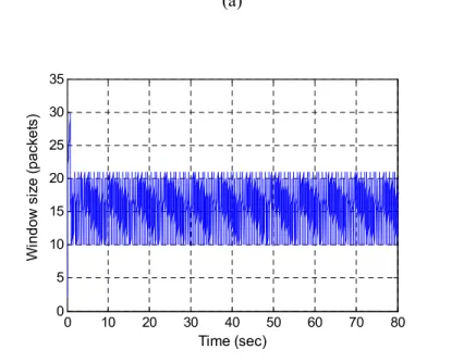
The waveforms of the window size for various time scales are shown in Figure 9. The proposed S-RED model and ns-2 simulation results are quite similar, especially during the steady-state.

Figure 10 shows waveforms of the average queue size for various time scales. The average queue size in the S-RED model is approximately one packet larger than the average queue size resulting from the ns-2 simulation results. This difference is due to the simplifications that we introduced in the S-RED model. Our S-RED model employs packet-marking/drop

probability calculated by Eq. (4), while the RED algorithm adopts a smooth drop probability pa

that increases slowly as the count increases:

b b a

p

count

p

p

⋅

−

=

1

where pb is the drop probability given by Eq. (4) and count measures the number of packets that

have arrived since the last dropped packet. In the S-RED model, pb is used as the final drop

probability and count is ignored. Since pb < pa, the average queue size of the S-RED model is

larger than that obtained via ns-2 simulations.

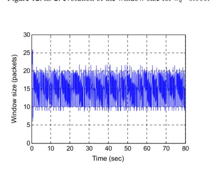
Figure 9. Evolution of the window size with default RED parameters: (a) S-RED model, and (b) zoom-in, (c) ns-2 simulation results and (d) zoom-in. Waveforms show good match between the S-RED model and the ns-2 simulation results.

(a) 0 10 20 30 40 50 60 70 80 0 5 10 15 20 25 30 35 Time (sec) W indow si ze ( pack e ts )

(b) 40 41 42 43 44 45 46 47 48 49 50 0 5 10 15 20 25 30 35 Time (sec) W indow si ze ( pack e ts ) (c) 0 10 20 30 40 50 60 70 80 0 5 10 15 20 25 30 35 Time (sec) W ind ow s ize ( packet s)

(d) 40 41 42 43 44 45 46 47 48 49 50 0 5 10 15 20 25 30 35 Time (sec) Wi n dow si ze ( p ac ket s)

Figure 10. Evolution of the average queue size with default RED parameters: (a) S-RED model and (b) zoom-in, (c) ns-2 simulation result and (d) zoom-in. The average queue size obtained using the S-RED model is higher than the average queue size obtained using ns-2 simulations.

(a) 0 10 20 30 40 50 60 70 80 0 1 2 3 4 5 6 7 8 9 10 Time (sec) A ver a ge queu e s iz e ( pack e ts )

(b) 40 41 42 43 44 45 46 47 48 49 50 5 5.5 6 6.5 7 7.5 8 Time (sec) A ver a ge queu e s iz e ( pack e ts ) (c) 0 10 20 30 40 50 60 70 80 0 1 2 3 4 5 6 7 8 9 10 Time (sec) A ver age q ueue si ze ( p ac ket s)

(d) 40 41 42 43 44 45 46 47 48 49 50 5 5.5 6 6.5 7 7.5 8 Time (sec) A ver a ge que ue s ize (pack e ts )

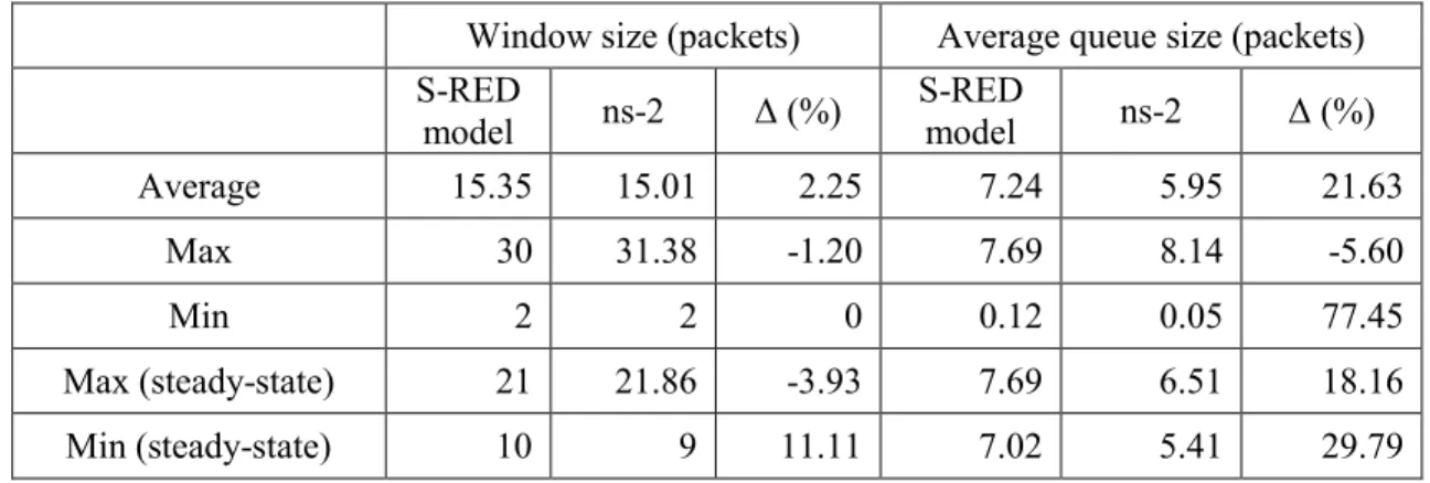
Table 2 summarizes the statistic values of the two state variables: window size and average queue size. It also compares the results with the ns-2 simulation. We calculated the average, maximum, and minimum values of the window size and average queue size over the duration of the simulation. In addition, the maximum and minimum values during the steady-state are also computed. We observed that the window size obtained from the S-RED model is similar to that obtained via the ns-2 simulation. The difference of the average queue size is approximately one packet.

Table 2. Statistic values of state variables for S-RED model and ns-2.

Window size (packets) Average queue size (packets)

S-RED model ns-2 ∆ (%) S-RED model ns-2 ∆ (%) Average 15.35 15.01 2.25 7.24 5.95 21.63 Max 30 31.38 -1.20 7.69 8.14 -5.60 Min 2 2 0 0.12 0.05 77.45 Max (steady-state) 21 21.86 -3.93 7.69 6.51 18.16 Min (steady-state) 10 9 11.11 7.02 5.41 29.79

4.3.2

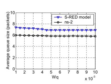
Validation for various queue weights

w

In order to evaluate the S-RED model for various system parameters, we varied the queue

weight wqbetween 0.001 and 0.01. The window size and the average queue size obtained from

S-RED model are compared to those from ns-2 simulation. The window size of S-S-RED model and

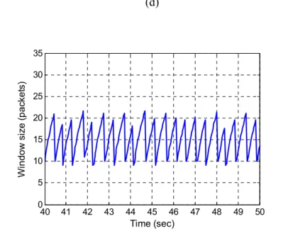
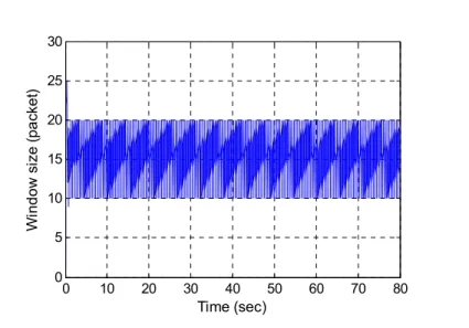
ns-2 are similar. For example, Figures 11 and 12 show the waveform of the window size, for wq=

0.006, for S-RED model and ns-2, respectively.

Figure 11. S-RED model: evolution of the window size for wq= 0.006.

0 10 20 30 40 50 60 70 80 0 5 10 15 20 25 30 Time (sec) W ind ow s ize ( p a cket )

Figure 12. n