The implementor/adversarial algorithm for cyclic and robust scheduling problems in health-care
Matias Holte Carlo Mannino
The implementor/adversarial algorithm for cyclic
and robust scheduling problems in health-care
Matias Holte
SINTEF ICT, Norway
Dept. of Applied Mathematics
[email protected]
Carlo Mannino
Sapienza
University of Rome
Dept. of Computer and System Sciences
[email protected]
January 31, 2011
Abstract
A general problem in health-care consists in allocating some scarce medical resource, such as operating rooms or medical staff, to medical specialties in order to keep the queue of patients as short as possible. A major difficulty stems from the fact that such an allocation must be established several months in advance, whereas the exact number of patients for each specialty is an uncertain parameter. Another problem arises for cyclic schedules, where the allocation is defined over a short period, e.g. a week, and then repeated during the time horizon. Even if the demand is perfectly known in advance, the number of patients may vary from week to week. We model both the uncertain and the cyclic allocation problem as adjustable robust scheduling problems. We develop a row and column generation algorithm to solve this problem: this turns out to be the implementor/adversarial algorithm for robust optimization recently introduced by Bienstock for portfolio selection. We apply our general model to compute master surgery schedules for a real-life instance from a large hospital in Oslo.
Keywords: Health-care optimization, Master surgery scheduling, Robust opti-mization, Mixed-integer programming.
1
Introduction
Mathematical optimization is playing an increasingly relevant role in health-care management ([14]). Indeed, as observed in [1], ”in the near future public resources for public health will become inadequate. Therefore, we need effective ways for planning, prioritization and decision making”. The major task of hospital adminis-trations is that of efficiently allocating a number of medical resources for different purposes. A large variety of assignment and scheduling problems arise: we refer the reader to [7] and [14] for several examples and approaches.
The allocation of resources to different medical specialties is directly connected to the admission planning problem, which amounts to establishing the sequence of accepted patients. Typically, patients requiring some specific therapy are first placed in a waiting list and thereafter admitted to the hospital. A standard performance indicator for hospital efficiency is related to the length of such lists. Shorter lists are obviously preferred, but it is in general impossible to avoid a certain amount of queue, and maybe not even desirable. Indeed, the absence of queue for some specialties could actually reveal an inefficient allocation of some scarce resource.
It follows that the demand for medical care is met not only by scheduling the necessary resources but also by allowing a certain amount of queue. Albeit a short waiting list may be acceptable, long queues are to be avoided, as they represent a huge cost for health-care systems ([9],[13]). For each specialty, the cost of its queue is a design parameter which must be established by the hospital board. In the typical case, the cost will be represented by a convex function, with marginal costs increasing with the queue length.
So, a basic scheduling problem in health-care may be stated as the problem of allocating a number of resources to medical specialties so as to minimize the queue costs.
Clearly the allocation process must be undertaken long in advance and may involve some negotiation. So, resources are allocated at the beginning of a time horizon which may be quite long - from months to years. The number of patients for each specialty is thus estimated in advance and the actual number may differ substantially from the initial guess. In addition, schedules are often calculated with reference to the planning horizon (e.g. from one to four weeks) and then cyclically repeated along the much longer time horizon: obviously the actual demand may vary
from period to period, even if deterministically known in advance. A safe schedule should then ensure that queues are as small as possible when the demand is the worst possible (with respect to the chosen schedule).
This kind of problems can be tackled by robust optimization (see [3]). In the robust optimization paradigm, the parameters of the problem (i.e. the coefficients of the constraint matrix and the right hand sides) are not completely specified and they may vary in the so called uncertainty set. One wants to find a value for (all of) the decision variables which is feasible for any possible realization of the parameters in the uncertainty set. A slightly different version of the robust optimization paradigm, which however may have relevant practical and theoretical consequences ([3]), is theadjustable robust counterpart of an optimization problem. This variation was introduced to take into account the presence in the model of
adjustablevariables, i.e. ”variables which do not correspond to actual decisions and can tune themselves to varying data” [4].
In our contest, we assume that the demand for medical care in the different specialties is an uncertain parameter and may vary within a given set Y. Also, in the optimization model we have variables associated with the schedule and variables associated with the queues. While the schedule variables represent ”here and now” decisions, the queue variables ”adapt” to meet the actual demand. In other words, the feasible schedules are those for which, for any possible demand realization,there exists a queue value so that the demand is met. We make explicit use of this def-inition in devising the cutting plane algorithm for the robust scheduling problem described in Section 4. It turns out that the resulting approach can be interpreted as theimplementor-adversary algorithm for robust optimization introduced by Bi-enstock in [6]. In the same paper, BiBi-enstock also claims to expect that similar ideas would prove useful for other robust optimization models. In this paper we confirm his forecast.
We apply our technique to instances of the Master Surgery Scheduling (MSS) Problem, a much addressed and studied problem in the class of scheduling prob-lems in health-care. The literature on the deterministic version of this problem is quite huge; a comprehensive survey on the topic can be found in [7]. In contrast, few papers deal explicitly with uncertainty. In [2], [9] and [12], the authors apply mathematical programming and local search techniques to cope with stochastic du-rations of surgical procedures. Two recent papers deal with uncertain demand, but with different assumptions and, consequently, different solution approaches. In [2], a probability (multinomial) distribution of the demand is given and the corresponding stochastic problem is modelled as a mixed integer linear program. In contrast, in [11] no probability distribution on the demand is known, which instead is assumed to vary in a given interval, and a light robustness model ([8]) is constructed to find
suitable schedules.
The overall approach has been successfully applied to real-life instances provided by SAB (Sykehuset Asker og Bærum HF), a major hospital in the city of Oslo.
2
The master scheduling problem
In this section we formalize the general scheduling problem with queue cost mini-mization in health-care. Let G be the set of specialties, such as orthopedics, gyne-cology, etc.. We denote by D the set of days in our planning horizon, while R is the set of available medical resources, e.g. rooms or surgical teams, or even feasible combinations of medical resources. We assume here that medical resources can only be assigned by an integer number of time slots1. Depending on his/her specific treat-ment, each patient requires a set of contiguous time-slots of the medical resource, calledblock. In the deterministic model, the overall block demand in the time hori-zon, for each specialtyg ∈Gand each possible block lengthl ∈L, is a non-negative integer bgl. In what follows, we indicate by bg ∈Z+G the vector (bg1, . . . , bg|L|)T, and
by b ∈ Z+G×L the vector (bT1, . . . , bT|G|)T . Finally, observe that ll·bgl is the total amount of slots required for specialty g during the time horizon. The number of time slots available in each day may vary from day to day. To simplify the notation let us introduce the set ofsuperslots S, namely the set of feasible unordered triples {r, s, d}, where r is a medical resource,s a time-slot andd a day. That is, superslot {r, s, d} ∈ S if resource r is available at slot s in day d. In this setting, a ( su-per)block is simply a subset B ⊆S such that the superslots in B correspond to the same medical resource, to the same day and to one or more contiguous time-slots. Finally, letqgl denote, for each specialtyg and each block lengthl, the queue length measured as the number of unscheduled patients. We denote byqg ∈Z+G the vector (qg1, . . . , qg|L|)T, and by q ∈ Z+G×L the vector (qT1, . . . , q|TG|)T. A major task of the
hospital board is to be able to keep short queues. Long queues have a social cost as wait times can impact health outcomes. We model such cost as a function f
decomposable in the different specialties and block lengths, i.e. f(q) =g,lfgl(qgl), where fgl is a non-decreasing, convex and piece-wise linear function. So the basic
Master Scheduling Problem amounts to finding a feasible assignment of superslots to each specialty (Master Scheduleor (MS)), so as to minimize the queue cost f(q).
Cyclic Schedules. The MS prepared by the hospital planning department is typ-ically active for a long period, normally from one to a few years. Such long duration is mainly motivated by the fact that finding a MS is a difficult task, which involves
specialized personnel for several working days. In addition, the hospital staff is af-fected by such timetable and the employees can put up a significant resistance to changes to the actual configuration.
In contrast, the actual planning horizon is much shorter, typically from one to eight weeks. The MS calculated for the planning horizon is then used as a pattern and repeated for the whole period of validity. So, the full MS which may hold for years is actually obtained by taking M copies of a shorter MS which refers to a few weeks. Again the reason to this is manyfold, but one major fact is that people prefer to have repeated working patterns along the year(s). Despite of the fact that the MS stays unchanged from period to period, the projected demand in each period may vary. Consequently, queue lengths and queue costs will also vary from period to period. Let us denote by bi ∈ Z+G×L the (projected) demand in period
i, for i = 1, . . . , M, and let Y = {b1, . . . , bM} be the set of all demand vectors. An interesting goal is now that of finding a MS which is valid for all periods, and such that the largest queue cost is minimized. That is, denoting by qi ∈Z+G×L the queue vector in period i= 1, . . . , M, the cyclic MS problem (c-MS) is the problem of finding a MS such that the quantity maxif(qi) is minimized.
Robust Schedules. The queue length depends both on the MS and on the de-mandb, which in turn is typically estimated from historical records. However, such estimate is inherently uncertain, and we assume that, for eachg ∈Gand l ∈L, the quantity bgl may vary between two possible values, namely
βgl ≤bgl ≤γgl (1)
As observed in the seminal paper by Bertsimas and Sim [5], in most realistic situations it is very unlikely that all uncertain parameters assume simultaneously their upper bounds. In [5] this observation is exploited by assuming that only a given number of the uncertain coefficients may deviate simultaneously from the reference value. This restriction does not look appropriate in our case. Instead we assume here that, even if in principle all demandsbgl may vary within the corresponding feasible interval, still the overall number of slots required by all patients in the different specialties does not exceed a threshold K, i.e.
g
l
l·bgl ≤K (2)
Again, we denote byY ={b1, . . . , bM}the (finite) set of feasible demand vectors, namelyY ={b ∈ZG×L:b satisfies (1) and (2)}.
Now, as in the c-MS problem, we want to find a MS which minimizes the largest queue cost. If we denote by qi ∈ Z+G×L the queue vector with respect to bi ∈ Y, then the adjustable robust MS problem (aR-MS problem) amounts to finding a MS such that the quantity maxif(qi) is minimized. It should be apparent that the c-MS problem and the aR-MS problem only differ in the way the set Y is defined, and from the next section we unify the discussion.
3
An adjustable-robust model for the MS
prob-lem
There are several alternative ways to represent the MS problem by mathematical optimization models, and in particular by mixed-integer linear programs (MILPs) (see [1] for various examples). Here we adopt the so called pattern formulation
introduced in [11] for the master surgery scheduling problem. Such formulation is based on the concept of l-pattern, which is simply a set of l contiguous superslots corresponding to the same day and the same medical resource. For example, if the slot length is 2hand a working day is 8h, then we have 4 time-slots. Correspondingly, we have four different 1-patterns (patterns of one slot or 2 hours), three distinct 2-patterns (4 hours), 2 distinct 3-2-patterns (6 hours) and one 4-pattern (8 hours).
When a specialty is assigned a block of lengthl, it is actually assigned a specific
l-pattern. Observe that each pattern corresponds to a precise time interval (i.e. from 10:00 to 16:00). Each specialtyg ∈G”asks” for a number bgl of patterns with block length l, for each possible block length l. Let us denote by P the set of all possible patterns, and let E = {{u, v} : u, v ∈ P and u∩v =∅}, i.e. E is the set of non-disjoint pair of patterns. In other words, {u, v} ∈ E if and only if pattern
u and pattern v (which are both collections of time contiguous superslots) share a common superslot. Thus, two patterns intersect if they correspond to the same medical resource and they overlap in time. For all g ∈Gand p∈P we introduce a binary variablexgp which is 1 if and only if pattern pis assigned to specialty g. To simplify the notation in the basic model we assume that every pattern p ∈ P can be assigned to any specialty g ∈G. It is not difficult to extend the model to cope with infeasible assignments by fixing suitable variables to 0. This may be the case, e.g., when a specialty needs some specific equipments not available in all operation rooms.
Letp, q ∈P be two (not necessarily distinct) patterns. If p and q intersect (i.e. {p, q} ∈E) then they cannot be assigned simultaneously. This is represented by the following packing constraint:
xfp+xgq ≤1, g, f ∈G,{p, q} ∈E, g =fp=q (3) Similar packing constraints may be included to represent other incompatible assignments, but we omit here the discussion for sake of brevity. A vector x ∈
{0,1}G×P satisfying all above inequalities is a Master Scheduling (MS) (or Master Schedule). The set of all feasible MS is denoted byX.
Actually, as shown in [11], the above constraints can be strengthened by consid-ering any setC of mutually intersecting patterns. Then we can replace (3) with the following family of inequalities:
g∈G
p∈C
xgp≤1, C ∈ C (4)
whereC is the family of the maximal sets of mutually intersecting patterns. Such a family can be identified efficiently ([11]).
Now, let P(l) be the set of patterns of length l. The quantity p∈P(l)xgp is the number of blocks of length l assigned to specialty g: in principle this quantity may exceedbgl. Then the queue qgl of patients of group g with block length requirement
l is defined as:
qgl = max(0, bgl −
p∈P(l)
xgp) g ∈G, l ∈L (5)
Thus, the queue q∈Z+G×L is a non negative function q(x, b) of the MS xand of the demand b.
The convex piece-wise linear cost associated with q can be easily transformed into a linear one by introducing suitable variables and constraints ([11]).
For sake of simplicity we discuss here the simpler case of a linear cost function. In particular, we consider the cost c(q) of the queue q to be proportional to the queue total length, i.e.
c(q) = g∈G
l∈L
cgl·qgl (6)
wherecglis a suitable, strictly positive constant (see Section 5 for the exact definition of the cost vector c in our test cases). The extension to the more general convex, piece-wise linear case is straightforward.
By associating a non-negative real variable sgl with qgl, for g ∈ G, l ∈ L, the (deterministic) MS problem can be formulated as following Mixed Integer Linear Program (MILP): min ξ s.t. (i) g∈Gp∈Cxgp ≤1, C ∈ C (ii) sgl +p∈P(l)xgp ≥bgl, g ∈G, l ∈L (iii) ξ ≥g∈Gl∈Lcglsgl ξ ∈IR, s∈IRG+×L, x∈ {0,1}G×P (7)
Constraint (7.ii) along with the non-negativity ofsensure that, for anyx andb, we haves≥q(x, b). Moreover, thanks to (7.iii) and the structure of the cost coefficients which are strictly positive, we trivially haves∗ =q(x∗, b) for every optimal solution (x∗, s∗) to (7).
Cyclic and Robust Schedules. We assume now that the demandb can actually range in the setY previously defined, that we rewrite for the reader:
Y :={b∈ZG×L :βgl ≤bgl ≤γgl, g l l·bgl ≤K}={b1, . . . , b|M|} (8)
whereβ and γ are non-negative vectors. Then the aR-MS problem can be stated as the following min-max problem:
min
x∈X maxb∈Y c(q(x, b)). (9)
Following Bienstock ([6]) we can interpret this problem as a particular imple-mentor/adversarialgame, where the implementor establishes a MS ¯x∈X trying to minimize the queue cost while the adversarial fixes a demandb ∈Y, this time max-imizingthe queue cost w.r.t. the schedule ¯x. We come back on this interpretation later on.
For every x ∈ X, let us denote by qi = q(x, bi) the queue when the demand vector is bi, for bi ∈ Y. As for the deterministic case, we associate a non-negative
real variable sigl with qigl, for every g ∈ G, l ∈ L and i ∈ M. Then the aR-MS problem can be immediately represented by the following MILP:
min ξ s.t. (i) g∈Gp∈Cxgp ≤1, C∈ C (ii) sigl+p∈P(l)xgp≥bigl, g ∈G, l∈L, i∈M (iii) ξ≥g∈Gl∈Lcglsigl i∈M (iv) ξ∈IR, s∈IR+G×L×M, x∈ {0,1}G×P (10)
In fact, constraints (10.ii) and non-negativity ensure that si ≥ qi, for i = 1, . . . , M, whereas constraints (10.iii) ensure that ξ ≥ maxi∈McTsi ≥ maxi∈M c(qi) with equality holding for the optimal solution. A major difficulty with the above formulation is the large number (possibly exponential in |G| · |L|) of inequalities (10.ii) and (10.iii) and variables sigl. A classical technique to cope with it is to ini-tially consider a small subset of such inequalities and variables and generate new ones only if necessary. This is the topic of the next section.
4
The implementor/advesary algorithm for the
adjustable-robust MS Problem.
We start by considering a subset ˜Y ⊆Y (corresponding to the set of indices ˜M ⊆M) and solve the (reduced) master problem
min ξ s.t. (i) g∈Gp∈Cxgp ≤1, C∈ C (ii) sigl+p∈P(l)xgp≥bigl, g ∈G, l∈L, i∈M˜ (iii) ξ≥g∈Gl∈Lcglsigl i∈M˜ (iv) ξ∈IR, s∈IR+G×L×M˜, x∈ {0,1}G×P (11)
Observe that the above problem contains in general fewer constraints and vari-ables than the original aR-MS problem (10) and it is easier to solve in practice. Now,
let (˜x,˜s,ξ˜) be the optimal solution to the current master problem. This provides a feasible MS ˜x. It is not difficult to see that, even if (11) contains in general fewer variables than (10), still ˜ξ is a lower bound on the optimal value of (10). Indeed, let us denote by ˆξ the optimal value to the proper relaxation of (10) obtained by dropping the constraints (10.ii) (10.iii) associated with the indices i ∈M \M˜. By definition, we have that ˆξ is a lower bound on the optimal value of (10): also, it is immediate to see that ˆξ = ˜ξ.
More in general, let ˜Y ⊆ Y¯ ⊆ Y, and let ˜ξ and ¯ξ be the optimal values to the master programs associated with ˜Y and ¯Y, respectively. Then, we have ˜ξ≤ξ¯.
Observe now that, for any bi ∈ Y˜, the queue cost c(q(˜x, bi)) is no larger than ˜ξ
(otherwisec(˜si)≥c(q(˜x, bi))>ξ˜, a contradiction). What happens to the queue cost if we let the demandbrange over the whole setY (and the schedule ˜xis unchanged)? In principle we may have a demand vectorbj ∈Y such that the corresponding queue cost c(q(˜x, bj)) is strictly larger than ˜ξ. However, if this is not the case, then the MS ˜x is optimal for the original min-max problem (9).
The above discussion can be summarized by following proposition:
Proposition 4.1 Let (˜x,s,˜ ξ˜)be the optimal solution to the current master problem (associated with Y˜ and M˜ ) and, for any bk ∈Y, let qk =q(˜x, bk) be the associated queue vector. Ifc(qk)≤ξ˜for allk ∈M, then(˜x,s,˜ ξ˜)can be extended to an optimal solution (˜x, s,ξ˜) of the original aR-MS formulation (10) with the same cost ξ˜.
Proof.
All we have to do is to let skgl =qglk for k∈M \M˜ and sigl = ˜sigl for i∈M˜. It is immediate to see that the solution (˜x, s,ξ˜) is feasible for (10).
So, if the conditions of the above proposition are satisfied, we do not need to solve the overall problem (10) and the current optimal vector ˜x is an optimal MS. Otherwise there exists ˆb ∈ Y \Y˜ such that c(q(˜x,ˆb)) >ξ˜, we let ˜Y = ˜Y ∪ {ˆb} and solve the associated master program once again.
In order to test if the conditions of Proposition 4.1 are satisfied or to identify a demand vector ˆb ∈ Y violating such conditions we set up a suitable MILP. In particular, we look for a demand vector b∗ ∈ Y maximizing the cost of the queue
q∗ =q(˜x, b∗). Ifc(q∗)>ξ˜thenb∗ is the required demand vector, otherwise c(qk)≤ξ˜
To this end, we can solve the following mixed integer non-linear program: max g∈Gl∈Lcglwgl s.t. (i) wgl = max(0, ygl−p∈P(l)x˜gp) g ∈G, l∈L w∈IRG×L, y∈Y (12)
The non-linear constraints (12.i) ensure that w = q(˜x, y), i.e. w is the queue associated with the demand vectory∈Y (and MS ˜x). In order to linearize constraint (12.i) we cannot proceed as for the master problem simply by introducing a suitable slack variable, because of the specific form of the objective function in (12). Instead we introduce, for each g ∈ G, l ∈ L, a binary variable zgl which is 1 if ygl −
p∈P(l)x˜gp < 0, and 0 otherwise. Then we substitute each constraint (12.i) with
the following linear constraints:
(i) wgl ≤Qzgl+ygl −p∈P(l)x˜gp (ii) wgl ≤Q(1−zgl)
(iii) wgl ≥0
(13)
where Q is a suitable large constant. In fact, if zgl = 1 then (13.i) becomes redun-dant, while (13.ii) and (13.iii) implywgl = 0. On the other hand, when zgl = 0 then (13.ii) becomes redundant while (13.i) becomes
wgl ≤ygl−
p∈P(l)
˜
xgp.
Finally, the strictly positive coefficients in the objective function implies thatwgl =
ygl−p∈P(l)x˜gp in every optimal solution to the linearized version of (12).
The implementor/adversarial algorithm. We come back now to the relation between our column and row generation approach and the implementor/adversarial (I/A) algorithm for robust optimization proposed by Bienstock [6].
The I/A algorithm solves a problem of the form
F∗ = min
and can be summarized as follows:
Implementor/Adversarial Algorithm
Output: values L and U with L ≤ F∗ ≤ U, and x∗ ∈ X such that L = maxy∈Y f(x∗, y).
Initialization: Y˜ =∅, L=−∞, U = +∞.
Iterate:
1. Implementor Problem: solve minx∈Xmaxy∈Y˜ f(x, y), with solutionx∗. Reset L←maxy∈Y˜ f(x∗, y)
2. Adversarial Problem: solve maxy∈Y f(x∗, y), with solution y∗. Reset
U ←min{f(x∗, y∗), U}.
3. Test: IfU −L is small, exit, else reset ˜Y ←Y˜ ∪ {y∗} and go to 1. It is immediate to verify that the implementor problem at Step 1 of the above algorithm coincides with the master problem (11) associated with the set ˜Y. We have already observed that the optimal value of the master program can only increase as the set ˜Y gets larger, since the minimization problem becomes increasingly more constrained. This is why at Step 1 we can always update the lower bound L with the optimal value of the current master program. In contrast, the solution of the adversarial (slave) problem at Step 2 depends on the current master solution x∗
and, though always providing an UB for the original problem, such value can change unpredictably from one iteration to the next.
Speeding up the I/A algorithm. For our instances, the adversary problem is a relatively small integer program, which is actually solved quite efficiently by any commercial solver or by dynamic programming. In contrast, the implementor prob-lem is the large MILP (11) and most computing time is spent for its solution. However, we do not lose much by temporarily replacing program (11) with its linear relaxation. In fact, if we denote by ¯x the optimal fractional solution to the relaxed problem (11) and by ¯ξ its value, then it is not difficult to see that:
• ξ¯is a proper lower bound for the overall min-max problem (9) and Lcan still be updated as at Step 1 of the I/A algorithm.
• the adversarial problem maxy∈Y f(¯x, y) can still be defined and solved using the fractional solution ¯x: indeed its optimal solution y∗ is a valid demand vector (i.e. y∗ ∈Y). In contrast, its value is not (in general) an upper bound for the overall min-max problem, since ¯x is not a feasible schedule.
As observed in [6], a smart choice of the initial set ˜Y can significantly speed up the convergence of the I/A algorithm. So, solving an initial sequence of relaxed master problems, alternating with the corresponding adversarial problems, provides us an initial set of demand vectors in Y to populate ˜Y. This choice proved to be effective to reduce overall computational times, as shown in the next section.
5
Computational experience
Our experiments deal with the Master Surgery Scheduling Problem (MSS), which amounts to assigning operation rooms to surgical specialties (see [11] for a detailed description of the problem and of the corresponding pattern formulation). In all cases we have six surgery specialties, or groups, namely Gastroenterology (Group 1), General Cardiology (Group 2), Gynecology (Group 3), Medicine (Group 4), Ortho-pedics (Group 5), and Urology (Group 6). Each group (specialty) must be assigned a suitable number of slots of operation room in the planning horizon. Since each specialty typically corresponds to a single medical group or staff, we need to consider additional packing constraints to avoid that two simultaneous (but not intersecting) patterns are assigned to the same specialty.
The computational experience has two major purposes. Firstly, to evaluate our specific implementation choices and assess the quality of the algorithm. Secondly, to evaluate the capability of the approach to cope with practical real-life scheduling problems of medical resources in hospitals.
The algorithm was tested on a shared linux computer with 8 GB memory and eight 1.8MHz processors (but only one assigned to our process), using CPLEX 11.0 to solve the linear and integer programs, and the code was implemented inpython. For all our experiments, we let the objective function be the following convex piece-wise linear function of the queue q:
g∈G
l∈L
l·c(qgl)·qgl
where c(r) = 1 if 0 ≤ r ≤ 3 (0 ≤ r ≤ 1 for the artificial, smaller instance), and
c(r) = 3 otherwise. In other words, the marginal cost is larger for long queues; also, patients with longer operation durations are more costly. Other choices of the coefficients can of course be made by the hospital management to reflect specific priorities.
5.1
Experiments for algorithm assessment
This first set of experiments is designed to evaluate some implementation choices and the general behaviour of the algorithm. To this purpose we created a small data set, described in Table 1, corresponding to one week demand.
Block lengths
1 2 3 4 Total Patients Total Slots Patients group 1 5-7 2-5 3-5 0-1 10-18 18-36 group 2 4-5 1-3 1-3 4-7 10-18 25-48 group 3 2-3 5-6 1-3 2-4 10-16 23-40 group 4 2-3 4-6 0-0 2-4 8-13 18-31 group 5 3-5 5-6 2-4 1-2 11-17 23-37 group 6 4-7 3-4 3-5 1-2 11-18 23-38 Sum 20-30 20-30 10-20 10-20 60-100 130-230
Table 1: The small artificial data set.
The different specialities are given in each row whereas the demand for each block length is given in the columns labelled from 1 to 4. The two numbers separated by hyphen in each entry are lower and upper limits on the demand, respectively. The last two columns report, for each specialty, the total (minimum and maximum) number of patients and the total (minimum and maximum) number of slots required in the planning horizon, respectively.
The schedule considered a planning horizon of 1 week, with 5 days and 6 slots/day. The medical resources amounted to 5 rooms. Consequently, we have 150 superslots (= # days × # slots × #rooms) and correspondingly, 2700 decision binary vari-ables. For this experiment, we fixed the total slot demandK = 150. In a first run we evaluate the original version of the implementor/adversarial algorithm, that is at each iteration both master and slave problems are solved to integral optimality.
The results are plotted in Figure 1. The algorithm ran for 601 sec. and for 36 iterations in total. For each iteration we plot the lower bound returned by the implementor (lower dotted line) and the upper bound returned by the adversarial (upper solid line), respectively. The value computed at each iteration corresponds to a small cross. Remarkably, already after 294 sec and 22 iterations, the gap was reduced to less than 5%. Actually, the corresponding implementor solution was globally optimal, but we needed other 14 iterations to prove it. It is important to remark here that, at any iterationithe solutionxi produced by thei-th master pro-gram corresponds to a feasible schedule. So, when solving the following adversarial problem, we are actually computing the worst-case cost when the schedule is xi.
This cost is thus the UB depicted, for our tiny instance, by the small cross points in the upper line of Figure 1. It is not difficult to see that already in the very early iterations of the algorithm the returned schedules are quite good, even if later on in the process we also obtain much worse solutions. A similar behaviour was also observed in several experiments on random instances as reported in [10].
Finally, observe that the time required to solving the adversarial problem sums up to less than 4% of the overall running time. For this reason, we concentrated on the implementor implementation when striving for speed-ups.
0 10 20 30 40 50 60 0 100 200 300 400 500 600 700 optimal value seconds adversary implementor
Figure 1: Run plot: small instance. The lower line corresponds to the lower bounds returned by the implementor. The upper line shows the upper bounds returned by the adversary.
To this end, we tested the relaxed version of the algorithm, as described at the end of Section 4. Namely, we drop the integrality stipulation on thex variables in most of the implementor runs. Integrality is re-established when the current gap between lower and upper bound is 0 (recall however that the upper bound returned by the adversarial in the relaxed iterations is not a valid upper bound for the original problem, as the input schedule is not integral).
The figures show a speedup of 44% (similar speed ups were also obtained in our experiments on different instances, see [10]).
Finally, as suggested in [6], we have tried a different speed-up by partially pop-ulating the set ˜Y with a number of demand scenario before starting the I/A algo-rithm. Unfortunately, in our tests the overall behaviour of the algorithm did not benefit from this strategy as small improvements in the number of iterations were counterbalanced by increased running times (per iteration).
5.2
Real-life test case
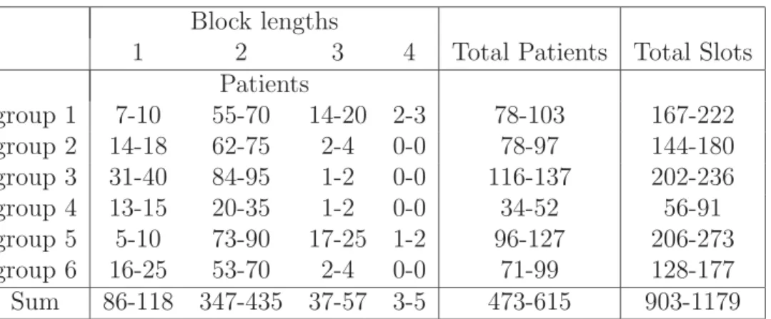
Our real-life test case refers to historical patient data from SAB, a major hospital in the city of Oslo (for a detailed description of such instances see [10] and [11]). The data are extracted from a three-year period. Namely, for each specialtyg ∈G and each possible block length l ∈ L, we consider the minimum mgl and the maximum value Mgl achieved in a 7 week-period (corresponding to our planning horizon) of the three years and select at random the lower boundβgl ∈[mgl, Mgl]. Similarly, we take the upper bound γgl at random in the interval [Mgl,1.5Mgl]. This is to cope with possible future increase in demand. The final scenario is summarized in table 2.
Block lengths
1 2 3 4 Total Patients Total Slots Patients group 1 7-10 55-70 14-20 2-3 78-103 167-222 group 2 14-18 62-75 2-4 0-0 78-97 144-180 group 3 31-40 84-95 1-2 0-0 116-137 202-236 group 4 13-15 20-35 1-2 0-0 34-52 56-91 group 5 5-10 73-90 17-25 1-2 96-127 206-273 group 6 16-25 53-70 2-4 0-0 71-99 128-177 Sum 86-118 347-435 37-57 3-5 473-615 903-1179
Table 2: Patient demand, real-life data set. Number of weeks and decision variables increased 7-fold compared to the small instance.
We choose a planning horizon of 7 weeks, with 5 days a week and 6 slots a day, giving 210 slots for the 6 groups. With 5 rooms available, this makes 1050 superslots available.
We run our tests for different values of the parameter K (the expected total demand of slots) ranging in the interval [925,1179].
Comparisons with the deterministic approach. The goal of robust optimiza-tion is to build prudent soluoptimiza-tions, that is soluoptimiza-tions which are intended to be protected
against the occurrence of the worst-scenario (w.r.t. the solution built). We use this criterium to compare our robust approach against the deterministic approach. The deterministic solution is obtained by solving the original scheduling problem w.r.t. a specific scenario chosen in the feasible setY. In particular, we consider two possible scenarios: one in which all demands are to their upper boundsγgl and one in which demands are at their average values (βgl+γgl)/2. Let us denote by xM and xA the corresponding optimal schedules.
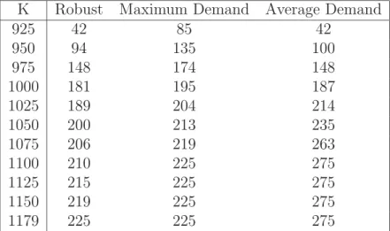
The results are shown in Table 5.2. For different values ofK (first column), the next three columns display the corresponding cost of the solutions generated by the three different approaches. In particular, for a given K, the corresponding entry in the columnRobust is the cost of the I/A solution with inputK. The next two costs on the same row are computed by running the adversarial problem with input K
and schedule xM and xA, respectively. The figures in Table 5.2 clearly show that the robust approach outperforms the other approaches.
K Robust Maximum Demand Average Demand
925 42 85 42 950 94 135 100 975 148 174 148 1000 181 195 187 1025 189 204 214 1050 200 213 235 1075 206 219 263 1100 210 225 275 1125 215 225 275 1150 219 225 275 1179 225 225 275
Table 3: Comparing the I/A algorithm against the deterministic approach with demand fixed to maximum and to average values
Also, for medium/high overall demand, the deterministic approach with maxi-mum demand seems to perform better than the deterministic approach with average demand, whereas the situation is reversed for low demand values.
The costs reported in Table 5.2 for the robust approach are computed by making the implicit assumption that the actual overall demand of slots is precisely K, i.e. the one we input to theI/A algorithm.
This is sometimes a too optimistic assumption, even if we may expect that hospital boards are able estimate the actual value ofK with reasonable confidence. A natural question is how the computed schedule behaves when the actual overall
demand differs from the estimated one. An answer is shown in Table 5.2, where the columns correspond to the different values of the input parameter K, whereas the rows correspond to the actual values of the demand. In particular, for each estimated
¯
K we compute the corresponding robust schedulexK¯ by the I/A algorithm. Then, for each possible overall demand ˜K ranging from 925 to 1179, we run the adversarial with input ˜K and schedule xK¯, to generate the worst-possible scenario. The final costs are reported in Table 5.2.
Actual Estimated K demand 925 950 975 1000 1025 1050 1075 1100 1125 1150 1179 925 42 53 68 55 63 88 106 73 85 115 85 950 100 94 119 109 108 133 151 121 132 160 135 975 148 151 148 148 154 151 171 172 166 182 174 1000 187 196 187 181 181 182 183 188 181 192 195 1025 221 235 206 202 189 194 196 195 194 197 204 1050 231 270 227 227 212 200 202 201 203 201 213 1075 243 296 237 237 223 212 206 206 208 207 219 1100 245 323 242 242 234 218 212 210 212 213 225 1125 245 329 243 246 239 222 216 216 215 218 225 1150 247 333 243 251 244 227 221 221 221 219 225 1179 247 336 243 257 245 230 225 225 225 225 225
Table 4: Solution values for different values of estimated and actual overall demand.
Not surprisingly, the above table shows that, for a given value of the actual demand the minimum cost is achieved when it equals the estimated one (diagonal entries in bold). Most important, the table shows that when the estimated demand is close to the actual one, then the solution cost does not increase too much. In particular, in most cases it is preferable to overestimate rather than underestimate. Observe that the ratio between the largest and the smallest entry in a row can be quite large (over 100% in some cases). This means that a non-careful planning can actually be very costly for a hospital, if a worst-case scenario occurs.
Concluding, this experiment shows that if the hospital estimates are reasonably close to the actual demand, then our approach is able to generate safe solutions.
References
[1] Beli¨en J., Exact and heuristic methodologies for scheduling in hospitals: prob-lems, formulations and algorithms. PhD Thesis, Faculty of Business and Eco-nomics, Katholieke Universiteit Leuven, 2006.
[2] Jeroen Beli¨en and Erik Demeulemeester. Building cyclic master surgery sched-ules with leveled resulting bed occupancy. European Journal of Operational Research, 176(2):1185–1204, 2007.
[3] Ben-Tal A., El Ghaoui L. and Nemirovski A., Robust optimization methodology and applications. Mathematical Programming, 92(3):453–480, 2002.
[4] Ben-Tal A., Goryashko A., Guslitzer E. and Nemirovski A., Adjustable robust solutions of uncertain linear programs. Mathematical Programming, 99(2):351-376, 2004.
[5] Bertsimas D. and Sim M., The Price of Robustness. Operations Research, 52(1):35–53, 2004.
[6] Bienstock D., Histogram models for robust portfolio optimization. J. Compu-tational Finance, 11:1–64, 2007.
[7] Cardoen B., Demeulemeester E. and Beli¨en J., Operating room planning and scheduling: A literature review.European Journal of Operational Research, 201 (3) 2010.
[8] M. Fischetti and M. Monaci. Light robustness. Book Series Lecture Notes in Computer Science, 5868(3):61–84, 2009.
[9] Hans E., Wullink G., van Houdenhoven M. and Kazemier G. Robust Surgery Loading. European Journal on Operational Research, 185 (3), 1038–1050, 2008. [10] Holdte M., A cutting plane algorithm for robust scheduling problems in
medicine Master ThesisUniversity of Oslo, 2010.
[11] Mannino C., Nilssen E.J. and Nordlander T.E.. A pattern based, robust ap-proach to cyclic master surgery scheduling. Journal of Scheduling, to appear. [12] J. M. Oostrum, M. van Houdenhoven, J. L. Hurink, E. W. Hans, G. Wullink,
and G. Kazemier. A master surgical scheduling approach for cyclic scheduling in operating room departments. OR Spectrum, 30(2):355–374, April 2008. [13] Patrick J., Puterman M.L. and Queyranne M., Dynamic Multipriority Patient
Scheduling for a Diagnostic Resource, Operations Research 56(6), 1507–1525, 2008
[14] Rais A. and Viana A., Operations Research in Healthcare: a survey, Interna-tional Transactions in OperaInterna-tional Research, 1–31, 2010.