AxleDB: A novel programmable query processing platform on FPGA

AxleDB: A Novel Programmable Query Processing Platform on FPGA

, Universitat Politcnica de Catalunya (UPC)- [email protected]

GORKER ALP MALAZGIRT, Bogazici University- [email protected] ORIOL ARCAS-ABELLA, Barcelona Supercomputing Center (BSC)

, Universitat Politcnica de Catalunya (UPC)- [email protected] ARDA YURDAKUL, Bogazici University- [email protected]

NEHIR SONMEZ, Barcelona Supercomputing Center (BSC)- [email protected]

With the rise of Big Data, providing high-performance query processing capabilities through the accelera-tion of the database analytic has gained significant attenaccelera-tion. Leveraging Field Programmable Gate Array (FPGA) technology, this approach can lead to clear benefits. In this work, we present the design and im-plementation of AxleDB: An FPGA-based platform that enables fast query processing for database systems by melding novel database-specific accelerators with commercial-off-the-shelf (COTS) storage using modern interfaces, in a novel, unified, and a programmable environment. AxleDB can perform a large subset of SQL queries through its set of instructions that can map compute-intensive database operations, such as filter, arithmetic, aggregate, group by, table join, or sort, on to the specialized high-throughput accelerators. To minimize the amount of SSD I/O operations required, AxleDB also supports hardware MinMax indexing for databases. We evaluated AxleDB with five decision support queries from the TPC-H benchmark suite and achieved a speedup from 1.8X to 34.2X and energy efficiency from 2.8X to 62.1X, in comparison to the state-of-the-art DBMS, i.e., PostgreSQL and MonetDB.

Additional Key Words and Phrases: Database Query Processing, Hardware Accelerators, Reconfigurable Computing

1. INTRODUCTION

In the rapidly growing field of Big Data, as the amount of data to manage increases, there is an increasing strain on Database Management Systems (DBMS) to meet high throughput and low latency requirements. The first main point of concern is the over-head of data movement that causes the throughput degradation, and decreasing the cache memory utilization per query. Secondly, conventional control-flow-based query processing engines can cause lower computational throughput compared to what can be achieved by application-specific hardware. From one side, to alleviate the overheads of data movement, one promising solution is to bring the computation closer to where the data resides, so that more operations can be completed avoiding non-essential data movement [1]. The gains are two-fold: easing the load on the host CPU for performing database operations, and reducing the negative impact on the performance of high-latency I/O operations. As a result, significant throughput improvements, as well as a reduction of I/O overheads can be achieved. On the other hand, streaming data through highly specialized hardware accelerators in a deeply pipelined fashion can significantly improve the computational throughput of the query processing engine.

FPGAs provide a unique opportunity to build an efficient query processing platform, by constructing a high-throughput execution engine with the additional aim of mini-mizing overheads of data movement. It is mainly the consequence of;(i)the inherent characteristics of massively parallel and configurable architecture of FPGAs, suitable for data streaming in deep pipelined-style execution (ii)the rise of High-Level Syn-thesis (HLS) technology, which makes FPGA applications relatively easier to develop compared to low-level languages such as VHDL or Verilog, and(iii)the availability of 1_{Behzad Salami is the corresponding author. Address: Nexus I Building, Office 303, Campus Nord UPC} Gran Capita 2-4, 08034, Barcelona, Spain

soft cores that implement modern interfaces, such as PCIe 3.0 (Peripheral Component Interconnect Express) or SATA-3 (Serial AT Attachment).

For the query processing, FPGAs have been utilized in two distinct approaches:(i) traditional data offloading mechanisms, where data in the host-attached storage is of-floaded towards external processing units or accelerators implemented in FPGA, or(ii) placing the processing units directly in the datapath between the host machine and the main storage units. The first approach could incur overheads stemming from the addi-tional data movement since data needs to be offloaded through Operating System (OS) and device driver layers [2], [3], [4]. In contrast, the second approach allows processing units to get direct access to data blocks and facilitates low-latency data transmission [5], [6]. Also, it can correspond to significant speedups in the query execution.

By introducing a novel architecture for managing data movement through hard-ware accelerators and storage, in this work, we present the design and implementa-tion of AxleDB. AxleDB is an FPGA-based engine that enables fast query processing by melding highly-efficient accelerators with commercial-off-the-shelf (COTS) storage using modern SATA-3, PCIe-3, DDR-3 (Double Data Rate) interfaces, in a novel, uni-fied, and a programmable environment. Tightly coupled with a Solid State Disk (SSD) that stores blocks of database tables, AxleDB is designed to execute complex Struc-tured Query Language (SQL) queries in full by performing various time-consuming query operations using specialized hardware accelerators, while the overhead of data movement between storage and compute units is also minimized. Thanks to the mas-sively parallel and pipelined architecture of FPGAs and efficiently exploiting its em-bedded modules, i.e., low-latency on-chip RAM and DSP blocks, AxleDB provides a diverse set of high throughput query processing units for performing filtering, arith-metic, aggregation, group by aggregation, table join, and sorting operations. Also, to reduce I/O transfers, AxleDB supports FPGA-based database indexing, which is an efficient method to perform a quick scan of large database tables [7]. AxleDB is con-nected through a fast PCIe-3 interface and managed by a host system. In the host machine, PostgreSQL [8] runs as the host DBMS, which was enhanced to manage the data and instruction flow. AxleDB can process complex SQL queries using an extensive set of query-specific instructions, which can be generated from a given SQL query in the host.

In a nutshell, the main objectives of AxleDB as a novel query processing engine, are:(i)to provide an infrastructure that sits between host and data storage in SSD, and utilizes PCIe-3 and SATA-3 interfaces to work directly with blocks of database columns,(ii)to design a set of efficient query accelerators inside such an infrastructure that can facilitate the query processing in a fully pipelined fashion(iii)to investigate the efficiency of a database indexing method in the proposed FPGA-based platform as a technique to I/O transmitting reduction, and (iv) to allow the DBMS to utilize these accelerators by issuing AxleDB special instructions, exposing flexibility in data movement and in enabling accelerators. More specifically, the contributions of this paper are as follows:

— We describe the unified AxleDB platform that includes query processing-specific ac-celerators that are coupled to the storage device. Also, the efficient data management mechanism of the AxleDB to control the flow of data, which effectively enables rapid query processing in the hardware.

— We present novel and efficient database query processing accelerators for filtering, arithmetic, aggregation, groupby aggregation, table join, and sorting operations, as well as a MinMax database indexing method to reduce the disk I/O transfer. Lever-aging them in a pipelined fashion leads to a high throughput query processing. To reduce the development time and to achieve more optimized designs we employed

modern HLS tools in various parts of the AxleDB. We explain our design decisions in detail while using Vivado HLS and Bluespec SystemVerilog.

— AxleDB is tailored for programmability and provides a diverse set of specific instruc-tions for data movement and query execution. These query-specific instrucinstruc-tions are generated at the host and used to program the AxleDB to process any given SQL query. For elaboration, we provide a step-by-step detailed query example from the commonly-used TPC-H benchmark.

— We evaluate the performance and energy efficiency of the AxleDB under various con-ditions, by running five decision-support TPC-H queries. We compare the AxleDB against the query processing engines of the state-of-the-art software-based DBMS, PostgreSQL, and MonetDB, in the single-threaded and multi-threaded modes. For the various class of the SQL queries, i.e., intensive, process-intensive, and I/O-process-balanced, we achieved speedups up to 34.2X and energy efficiency up to 62.1X, against the software DBMS.

The paper is organized into eight sections. Section 2 describes the architecture of the AxleDB by describing its major components. In Section 3 we illustrate the AxleDB by an example query to show how its components are utilized to process the exam-ple query. Section 4 introduces the supported database accelerators and the proposed database indexing method. The evaluation methodology is explained in Section 5. We discuss the experimental results in Section 6. Section 7 reviews the previous state-of-the-art query processing platforms, and finally, we conclude the paper in Section 8.

2. THE OVERALL ARCHITECTURE OF THE AXLEDB

In a relational DBMS, data is organized into tables, using a model of vertical columns and horizontal rows. The columns have a data type and a name. The rows represent entries in the database. The DBMS can store the data tables in two distinct models, row or column oriented storage. In column-oriented storage, all of the fields of a col-umn are serialized and stored together. As opposed to row-oriented storage, DBMS can lead to higher I/O throughput as it would not need to load unnecessary columns of data in a column-oriented fashion. Exploiting SQL queries, meaningful information can be extracted by processing the data that is organized in tables. For this aim, the core query processing engine, as the backbone of a DBMS, manages the actual processing of SQL queries, following an established query plan. However, other functionalities of DBMS such as user authentication, logging, security, concurrency, etc., can be handled by other corresponding components rather than the core query processing engine. In this work, we concentrate on the query processing part itself, by attacking the compu-tationally intensive query processing. We leave the other essential DBMS functionality for future work.

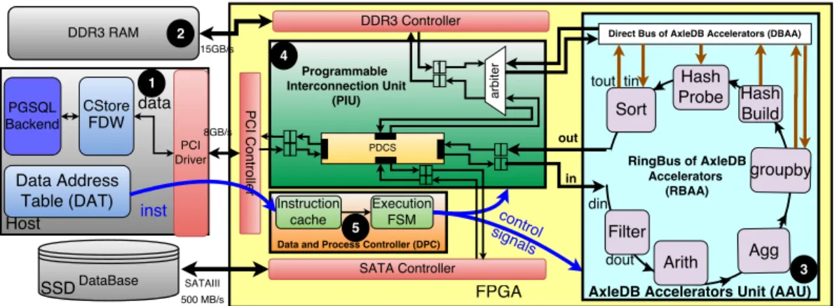
The main principle of the proposed database query processing platform, AxleDB, is to essentially move database computations closer to where the data resides, to obtain high performance in a flexible and programmable environment. Figure 1 shows the overall architecture of AxleDB. AxleDB resides between the host machine that runs the DBMS, and the database storage in an SSD. In the host, we primarily targeted to use PostgreSQL [8], one of the most popular open source relational DBMS. However, the infrastructure of AxleDB was designed to be software-agnostic and could be ported to other DBMS, e.g., MonetDB [9].

The host communicates with AxleDB through an Application Program Interface (API), to transfer data and instructions using the PCIe-3 interface. When the host ini-tiates the query execution, the query plan needs to be converted into AxleDB instruc-tions. Inside AxleDB, these instructions are managed and executed by the Data and

Process Controller (DPC), which orchestrates the movement of data blocks between SSD, DDR-3, host, and Accelerators. The query is effectively executed by streaming blocks of data, from the storage, through the accelerators, and back. Finally, the result of the query is returned to the software or stored back into the SSD. The architecture of AxleDB is composed of five major components:

(1) Software Extensions for DBMS in the host, including the Data Address Table (DAT) and the CStore Foreign Data Wrapper (FDW) extension of PostgreSQL, to manage the transfer of instructions and data, respectively. We provide detail infor-mation in Section 2.1.1.

(2) Data Storage Units, i.e., SSD, DDR-3, and host that are used as the primary or secondary database storage units and device controller cores, i.e., SATA-3, DDR-3, and PCIe-3 to manage the data transfer to/from storage units. We provide detail information in Section 2.1.2.

(3) AxleDB Accelerators Unit (AAU), which is a set of efficient DBMS query acceler-ators, i.e., filter, arithmetic, aggregation, group by, hash build, hash probe, and sort. To transfer data, accelerators are organized inside a ring bus, RingBus of AxleDB accelerators (RBAA), and a direct bus, DirectBus of AxleDB Accelerators (DBAA). We provide detail information about their overall interconnection in Section 2.1.3. Also, we introduce the internal structure of the accelerators in Section 4.

(4) Programmable Interconnection Unit (PIU) to set up a path to transmit the data in a fully flexible fashion. The PIU is composed of i) a 4-port bidirectional programmable data connection switch (PDCS) to exchange the data among SSD, DDR-3, host, and RBAA,ii)an arbiter to control the bandwidth sharing of DDR-3 by serializing its concurrent requests, and iii)a set of synchronizing First In First Out (FIFO) buffers for each individual port, separately for read and write directions, to cross the different clock domains. We provide detail information in Section 2.1.4.

(5) Data and Process Controller (DPC)that is composed of an Instruction Cache (IC) to locate the instruction set and an execute Finite State Machine (FSM)i)to manage the accesses to the off-chip data sources andii)to control the accelerators to execute the corresponding query, by issuing the appropriate control signals to the PIU and to the AAU, respectively. These signals are generated by translating instructions of AxleDB. We provide detail information in Section 2.1.5.

We elaborate the aforementioned components in Section 2.1, individually. 2.1. Major Components of AxleDB

In this section, we elaborate the architecture of AxleDB and describe the role of each constituting component, individually.

2.1.1. DBMS Software Extensions for AxleDB. The host communicates with AxleDB for two purposes:i)to access the database tables that reside in the SSD, andii)to pro-gram AxleDB using query-specific instructions in order to execute the SQL queries. In AxleDB, to process complex SQL queries, they first need to be translated to our specific instructions.2_{However, the certain currently unsupported operations, such as floating} point division (DIV), can utilize a fallback-to-host scheme, and instead be executed in the software extension of AxleDB. We use the CStore FDW extension of PostgreSQL to access the database tables [10], which we refer to as ’CStore’ for short. CStore man-ages data in a column-oriented format [11] that cause discarding unnecessary loads during the query processing and provides better I/O utilization. To transfer AxleDB 2_{The translation of SQL queries to AxleDB instructions is currently a manual process.}

Fig. 1: Overall architecture of AxleDB with its major components.(1)software exten-sions for DBMS in the host, (2) Data storage units and device controllers, (3) a set of efficient query processing accelerators, which is so-called AxleDB Accelerators Unit (AAU), (4) Programmable Interconnection Unit (PIU) to manage the accesses to the off-chip data storage units, in a fully flexible fashion,(5)Data and Process Controller (DPC) to orchestrate the involved modules of AxleDB to process SQL queries.

instructions, we use a shared memory region between the host and FPGA, called Data Address Table (DAT). DAT resides in the host memory and holds the list of instruc-tions of AxleDB and addresses of database tables. It is updated when the data tables are modified, or when a new query needs to be processed by AxleDB.

2.1.2. Data Storage Units and Device Controllers. AxleDB is connected to different sources of data, i.e., SSD, DDR-3, and host.i)As explained, the software extension of AxleDB is located on the host to initialize the configuration of the query execution, by issuing the query-specific AxleDB instructions. Its physical connection is through an PCIe-3 inter-face, with a maximum throughput of 8 GB/s. For this aim, we use Intellectual Prop-erty (IP) cores of Xilinx as the PCI-3 device controller.ii)SSD is connected through an SATA-3 interface, with a maximum throughput of 500 MB/s and is used as a pri-mary storage to resides the database tables. Furthermore, we use a modified version of Groundhog [12] as the SATA-3 device controller.iii)DDR-3 is used as the secondary storage, with a maximum throughput of 15 GB/s. It is used to locate the input/output data tables and the temporary tables, e.g., hash tables, during the query processing. Also, we use the Memory Interface Generator (MIG) IP core of Xilinx as the DDR-3 device controller.

To reduce the overheads of data movement, in addition to the techniques as men-tioned earlier, e.g., direct coupling of column-oriented SSD to the hardware accelera-tors, AxleDB is equipped with a database indexing method that is explained in Section 4.5.

2.1.3. AxleDB Accelerators Unit (AAU). In this section, we explain the overall organiza-tion and interconnecorganiza-tion of AxleDB accelerators. AxleDB is equipped with a set of hardware accelerators to carry out the query processing primitives, i.e., filter, arith-metic, aggregation, groupby, hash build, hash probe, and sort units. Each accelerator has i) an input data port to stream in input data (din), ii) an output data port to stream out the result data (dout), iii)an input signal to determine the state of the unit (state), which is elaborated later in this section, andiv)a set of inputs to define the functionality of the given accelerator, e.g., to define the filtering qualifiers in the

filtering unit. Also, some of them have additional ports to access the temporary data during the processing, i.e., hash tables in the groupby, hash build, and hash probe units, and partially sorted data set in the sort unit. For this aim, i)the groupby unit has input/output ports (tin,tout) to read/write the hash table,ii)the hash build unit has an output port (tout) to write into the hash table,iii)the hash probe unit has an input port (tin) to read the hash table, andiv)the sort unit has input/output ports (tin,

tout) to access the partially sorted data set. Other accelerators, i.e., filter, arithmetic, and aggregation units are inherently on-the-fly operations and do not need any access to the temporary data during the query processing.

To interface AAU with data storage units to transfer the input/output and temporary data set, the accelerators are connected through two distinct data buses, with respect to their sequential and random data access types. More specifically,i)the input/output data are usually accessed sequentially. Thus, the potential long latencies can be cov-ered by streaming data in a pipelined schema. Accordingly, to access the input/output data, our design decision is made due to providing a flexible schema. In contrast,ii)to access the temporary data, we set a shortcut path to DDR-3 with a minimum latency. Since the temporary data, i.e., hash table and partially sorted data, are accessed ran-domly, thus, a low-latency path would be efficient. We elaborate the interconnections, as below:

(1) RingBus of AxleDB Accelerators (RBAA):To build AxleDB flexible enough, we organize the accelerators inside a unidirectional ring structure that is so-called RBAA. We use the RBAA to only stream in/out the input/output data tables, and not temporary data, from/to the data storage units, i.e., SSD, DDR-3, and host, in a flexible schema. As it can be seen in Figure 1, the accelerators are chained to each other with a specific order, as follows: filter, arithmetic, aggregation, groupby, hash build, hash probe, and sort units. To set up the chain, we connect thedoutport of the earlier unit to thedinport of the latter unit, consecutively. Also, thedinport of the filter unit and thedoutport of the sort unit are used to externally interface the RBAA. Also, currently, we design RBAA as a single-channel bus, which leads to a single stream of data in the ring, at a time. Accordingly, to process an SQL query, we need to break it into a set of data streaming paths. By streaming data through the data paths, in a sequential order, as RBAA is a single-channel bus, processing of the corresponding SQL query can be accomplished. We will elaborate this process in Section 2.2 and also illustrate it for an example query in Section 3. (2) DirectBus of AxleDB Accelerators (DBAA):As mentioned earlier, groupby, hash build, hash probe, and sort units needs to be connected to an off-chip storage to ac-cess their temporary data set. For this aim, we use a dedicated data bus that is so-called DBAA. As it can be seen in Figure 1, thetin and/or tout ports of accel-erators are connected to this data bus. It is worth noting that accessing random data set, e.g., hash tables and partially sorted data set, under a long latency would cause a significant throughput degradation. Although, some techniques such as multithreading [22] can alleviate this issue, in the current version of AxleDB, our sort and hash-based accelerators are single-threaded. Alternatively, in AxleDB, we make some design decisions to decrease the latency of accessing the temporary data, by dedicating a direct data bus, as:

— We believe that DDR-3 is the only promising accommodation among the avail-able data storage units, i.e., SSD, DDR-3, and host, to cope with the temporary data. Since, DDR-3 has the shortest latency, which qualifies it for random data accesses such as hash tables and partially sorted data set. Thus, an intercon-nection to DDR-3 is designed for providing quick temporary data access of the aforementioned accelerators.

— Accessing DDR-3 through the ring bus incurs an additional latency (at max 7 cycles for each data access), which as explained, may cause performance degra-dation. Thus, to access the temporary data, we dedicate the direct bus, so-called DBAA without any additional latency. Similar to the RBAA, the DBAA is also a single-channel bus, which corresponds to transfer a single set of data, at a time. Also, as it is explained in Section 4.3 and 4.4, we substantially optimize the archi-tecture of the corresponding hardware accelerators by using the on-chip RAMs of FPGA to discard the latency of the temporary data access during the query pro-cessing.

In summary, we equip AxleDB withi)RBAA to provide flexibility to access the input and output data tables from various data storage units, andii)DBAA to quick access to the DDR-3 for some of the costly query operations, i.e., group by, hash build, hash probe, and sort units. The inherent advantage of having two distinct data buses is maximizing the overall throughput when various storage units are exploited for each data bus. For instance, by using SSD for the RBAA and DDR-3 for the DBAA, the bandwidth of both SSD and DDR-3, can be utilized, at a time. On the other hand, assuming that the RBAA is also connected to the DDR-3, the bandwidth of the memory needs to be shared among RBAA and DBAA. To share the bandwidth of DDR-3, we would need an arbiter that serializes the concurrent DDR-3 requests. The arbiter is a part of PIU, which we give more details on Section 2.1.4.

Nevertheless, in accordance to the SQL queries, a subset of the hardware acceler-ators are usually utilized at a time and not all of them. To meet this requirement in the hardwired chain structure of the RBAA, we design the accelerators to work in two distinct states:activeorsilent, which can be set by using an input signal. In theactive

state, the accelerators normally work, as expected to carry out the expected function of the query primitive, e.g., filtering, aggregating. In contrast, in the silentstate, the accelerators work as bypass buffers and only pass the incoming data to the next unit in the ring (with a single-cycle latency), without applying any function. As a consequence of this structure, depending on the SQL queries, we can utilize only the required subset of the accelerators, by setting them to the activestate and by setting other accelera-tors to thesilentstate. Considering the architecture, to access data, the chain incurs a latency of maximum 7 cycles. However, as mentioned earlier, we use it only for stream-ing input and output data tables and not for temporary data, which does not cause any throughput degradation. Because the additional latency is covered by streaming the sequential data access.

Note that the structure of the AAU may constrain supporting the SQL queries or achieving a fully optimal query plan of a given query. Below, we discuss the possible constrains of AxleDB:

(1) RBAA as a Hardwired Chain of the Accelerators:Although, the accelerators are chained inside a hardwired ring, the current order is viable enough to make an efficient query plan. Performing a filtering operation at the beginning can sig-nificantly reduces the size of the data for the next costly operations, i.e., group by, hash build, hash probe, and sort units, as they need frequent accesses to the off-chip DDR-3. In summary, by following this design point, the off-off-chip data accesses can be decreased, which in turn, corresponds to a significant throughput. We show more detail on this design point in Section 3.3 for an example query.

(2) DBAA as a Single-channel Data Bus:In the DBBA, only a single stream of data can use the bus, at a time. In other words, at a time, one of the corresponding accel-erators, i.e., group by, hash build, hash probe, and sort, can be active. Consequently, in an AxleDB-specific query plan for a given SQL query, we need to be ensured that each sub-query exploits only one of the aforementioned hardware units to access

random temporary data in DDR-3. We elaborate the query planning of AxleDB for an example query in Section 3.

However, this is not an optimal architecture, but it works for running complex queries in a fast and flexible way. Also, for any unsupported SQL queries, we can either i)if possible, rewrite the SQL query toward an equivalent and a more adapted version with AxleDB orii)call the software extension of AxleDB to process the query.

2.1.4. Programmable Interconnection Unit (PIU).PIU is designed to make AxleDB flexible enough to exchange the data among SSD, DDR-3, host, and RBAA. Also, it synchro-nizes the data movement among different clock domains and manages the bandwidth sharing. The PIU is composed of the following components:

— A 4-port Programmable Data Connection Switch (PDCS) to exchange the data blocks among SSD, DDR-3, host, and RBAA. To support all the possible data movement cases among the data sources, its ports are designed to be bidirectional, whereas each direction of each port can be utilized independently.

— The buffering and synchronizing FIFO modules to manage the data movement among the various ports of the PDCS. For the data transfer, buffering and synchro-nization is a crucial mechanism because, first, various data sources have different latencies, and second, they work with different clock frequencies. For each read and write direction, separate FIFOs are dedicated.

— An arbiter to manage the DDR-3 read/write requests, as DDR-3 has two distinct ac-cess modes, first, a direct connection from some of the accelerators in the DBAA to access their temporary data and second, an indirect connection through the PDCS to access the input/out data tables. In the arbiter, among the aforementioned current DDR-3 requests, we set the higher priority to the requests from direct con-nection DBAA to quickly serve the requests for the temporary data.

In summary, PIU is designed to efficiently share the bandwidth of the data storage units, while it can provide a fully flexible data movement schema.

2.1.5. Data and Process Controller (DPC) and AxleDB Instruction Set. DPC orchestrates the involved modules of AxleDB to process the complex SQL queries in a fast, efficient, and flexible schema. More specifically, it manages the movement of data and the activation of hardware accelerators to execute an SQL query, by issuing the control signals to the PIU and the AAU, respectively. Accordingly, the control signals from DPC, i) to the PIU determine the source and the destination of the data movement, and ii)to the AAU activate those accelerators that need to be utilized in the RBAA for any certain SQL query. Also, the parameters of each accelerator are determined by DPC, e.g., the filtering qualifiers for the filter unit.

The control signals are used by DPC to manage the query processing. They are gen-erated based on instructions of AxleDB. The query-specific AxleDB instructions are translated from the SQL queries in the host. Translation of the SQL queries to the instruction set of AxleDB is currently a manual process. We introduce instructions of AxleDB later in this section. As it can be seen in Figure 1, instructions are located in a shared location in the host memory that is called DAT. Then, they are sent to the IC that resides inside the DPC. The DPC fetches them from the IC, decodes, and executes by the execution FSM. Consequently, the control signals are issued and sent to the PIU and the AAU. Accordingly, the query execution is completed, when all the instructions inside the IC are consumed. In the end, the results of the query can be either stored back in the SSD or sent to the host. The DPC can now synchronize with the host and wait for more instructions to process a new query.

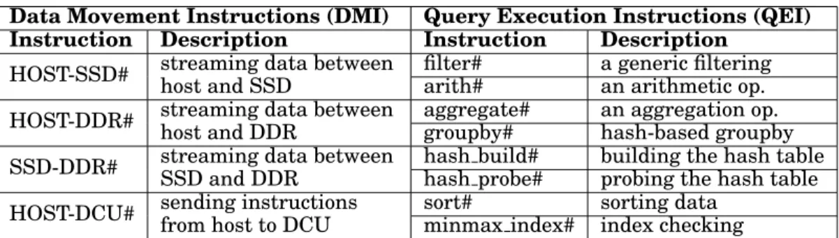
Table I: AxleDB instructions for data movement and query execution.

Data Movement Instructions (DMI) Query Execution Instructions (QEI) Instruction Description Instruction Description

HOST-SSD# streaming data between host and SSD

filter# a generic filtering arith# an arithmetic op. HOST-DDR# streaming data between

host and DDR

aggregate# an aggregation op. groupby# hash-based groupby SSD-DDR# streaming data between

SSD and DDR

hash build# building the hash table hash probe# probing the hash table HOST-DCU# sending instructions

from host to DCU

sort# sorting data

minmax index# index checking

Table I summarizes the instruction set of AxleDB for performing the tasks of data movement and query execution. Data Movement Instructions (DMI) set up the PDCS to exchange data blocks among the different sources of AxleDB, i.e., SSD, DDR-3, and host, bidirectionally. Furthermore, depending on the query plan, Query Execution In-structions (QEI) configure AxleDB to activate the corresponding accelerators in the RBAA to start streaming the input data. QEI consist of filtering, arithmetic, aggrega-tion, group by, hash probe, hash build, and sort instructions, as well as MinMax index creation/deletion instructions. Following by this way, AxleDB supports a large subset of the SQL queries, by mapping them to the architecture of AxleDB, which provided by using AxleDB instruction set. However, as mentioned earlier, the unsupported op-erations can be fallback to the software extension of AxleDB to accomplish the query processing. DMI and QEI include parameters, e.g., source, destination, key columns, carried column (payload), as well as accelerator-specific parameters, e.g., filtering op-erations (<, >, <>) and its qualifiers for the filtering unit.

2.2. The Execution Model of AxleDB

To alleviate the common restrictions of classical processor-based systems, the execu-tion model of AxleDB relies on the streaming of the data through the processing units. For this aim, FPGAs provide a unique opportunity, whereas their programmable logic blocks that are called LookUp Tables (LUT) can be chained together to construct deep pipelines. In this model, each processing node in the pipeline can be enabled, whenever the inputs are available.

To process an individual SQL query, we use AxleDB instructions to establish the required data streaming paths. In other words, in AxleDB, each SQL query is defined by a set of the data streaming paths. Source and destination of data, e.g., SSD, DDR-3, host, together with the required processing units in the AAU constitute a data stream-ing path. Accordstream-ingly, to process an SQL query, we need to make a query plan by breaking the SQL query to a set of sub-queries, considering the constraints of AxleDB’s structure that is discussed in Section 2.1.3. The generated sub-queries are one-by-one mapped to data streaming paths that can be run in AxleDB. Later on, we generate the required instructions and configure AxleDB to establish the corresponding data paths, sequentially. And finally, by streaming the data through the established data paths, the processing of the query can be accomplished. In the current version of AxleDB, at a time, we can establish a single data streaming path. This property leads to a se-quential, in order and one by one, execution model for the data streaming paths, which lead to having single stream of data in components of AxleDB, at a time.3_Accordingly, 3_{However, we believe that by adding parallel channels of data sources in the second version of AxleDB, it} can also support the parallel data streaming paths. This is an ongoing work.

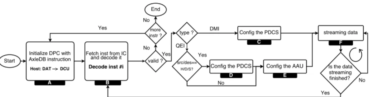
Fig. 2: The flowchart of the execution model in AxleDB. (In this figure: H= Host, S= SSD, and D= DDR-3.)

we elaborate the process of defining the data streaming paths by using instructions of AxleDB, i.e. QEI, DMI. The simplified flowchart of the execution model is shown in Figure 2. As it can be seen, first, the DPC is initialized by a set of AxleDB instructions that are copied from DAT in the host to the IC in the FPGA (A). Depending on the type of each valid instruction (B):

— DMI lead to exchange data among SSD, DDR-3, and host. Thus, after appropriately configuring the PDCS to set up the required source, destination, and direction, (C) the data are streamed in (F).

— QEI imply that data needs to be processed in the hardware accelerators, which lead to access the AAU. In the AAU, the corresponding accelerators are activated, and others are configured only to pass the data (E). Furthermore, for those QEI that need to transmit data to/from SSD, DDR-3, or host, which is determined by the parameters of the instructions, configuring the PDCS is also needed (D). Finally, data streaming is started through the established data path. As mentioned, at a time, we have a single stream of data in components of AxleDB. Thus, before reading new instruction, the current stream needs to terminate executing (F). Later on, we proceed to read the next instruction from IC (B) to start making the next data streaming path.

This process continues until consuming all the instructions of the IC while updating DAT with new instructions can restart the execution process of AxleDB.

3. ILLUSTRATING THE EXECUTION MODEL OF AXLEDB BY AN EXAMPLE QUERY

In this section, to demonstrate how AxleDB works, we illustrate the query processing procedure for an example query. The example query is Q03 from TPC-H benchmark [13]. AxleDB runs this query without any required modifications or code rewriting, where most of the accelerators presented in this work, are utilized. Since AxleDB is designed to be programmable, we can follow many different query plans to execute the queries. However, in this example, to show a comprehensive execution model of AxleDB, where input data is located in the SSD, we built a customized query plan. Accordingly, we first, load the input data from SSD to the DDR-3, and then, start query execution by retrieving data from DDR-3. In the rest of this section, we first, introduce the example query. Later on, show how AxleDB processes this example query by describing an optimal query plan, by introducing the list of the required AxleDB instructions to run the query plan, and by explaining how these instructions program the components of AxleDB to utilize the required modules.

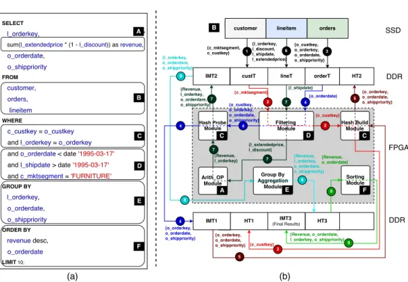
Fig. 3: (a) Example SQL query: Q03, (b) An example query plan of AxleDB to process Q03. To have a simpler figure,i)we partition the tables of the DDR-3 memory into two boxes at above and below of the FPGA, although, AxleDB is currently attached to a single channel of DDR-3, andii)we only show essential fields of the labels of arrows, excluding the input parameters of accelerators, payloads, etc.

3.1. Elaborating the Example Query

The example query is shown in the Figure 3 (a). In a typical SQL query, several lan-guage elements such asSELECT FROM,WHERE,GROUP BY, and ORDER BY

can exist. These operations can be semantically mapped to specialized hardware ac-celerators. In this example, theSELECTstatement fetches the desired data columns (l orderkey,revenue,o orderdateando shippriority)FROMthe given tables (customer,

ordersandlineitem). TheWHEREstatement is used to restrict the data in the tables and includes operations such as logical comparisons and arithmetic operations that filter the data relevant to the user (e.g.o orderdate <date 1995-03-17, l shipdate>

date 1995-03-17 and c mktsegment = FURNITURE). AxleDBs filtering units can be exploited to handle theWHEREclauses of SQL queries. When multiple tables are in-volved, the join statement (c custkey = o custkeyandl orderkey = o orderkey) is used to combine the data in these tables, based on a common field (custkeyandorderkey). This operation can be efficiently mapped to AxleDBs hash join accelerator. The GROUP BY statement aggregates data into groups based on a given field (i.e. l orderkey, o orderdate, o shippriority), which is mapped to AxleDBs hash-based groupby accel-erator. The ORDER BY statement sorts the data in ascending or descending order based on a given key (i.e.o orderdate, revenue), which can be performed using AxleDBs sorter accelerator. TheLIMITstatement causes to fetch a limited number of records. As it is further explained in Section 4.4, this operation is currently melded inside of AxleDBs sorter module.

3.2. How does AxleDB Process the Example Query?

To process an SQL query in AxleDB; first, the host generates a set of DMI and QEI. Currently, this is a manual process, but it can be automated by following a similar approach with Glacier [14]. Figure 3 (b) shows a simplified diagram for one possible query plan for processing the query Q03 on AxleDB, where the mapping from the key operations of the query to AxleDBs accelerators is indicated by letters (from A to F). To have a simpler figure, we did not show many details of AxleDB, i.e., RBAA, PDCS, instruction parameters, etc. Also, as it can be seen, the execution is accomplished in nine distinct steps. Each step is distinguished by using a set of arrows with its unique numbers and colors in the figure. The label of each arrow shows the key columns that are used in the corresponding part of the processing. Within each step, data can be streamed in a pipelined fashion, and between steps, it is sequential (in order and one by one), due to data dependencies.

Due to column-oriented data store format of AxleDB, only the 10 required columns out of a total of 33 columns (of three input data tables) are loaded from SSD to AxleDB. On the other hand, while loading data from SSD to DDR-3 memory, the columns of data are converted into batches that are appropriate for the processing units. Also, during the processing, different types of data can be stored in the DDR-3 memory, i.e., in-put data tables (custT, ordersT, lineT), intermediate data tables (IMT1, IMT2, IMT3), and temporary data tables, e.g., hash tables (HT1, HT2, and HT3). To access to the aforementioned data tables from the DDR-3, the memory bandwidth is shared. As ex-plained in Section 2.1.4, we manage bandwidth sharing by using an arbiter to serialize the concurrent memory requests. We elaborate it in Section 3.3 for a sample data path, step #7 as below, of the example query. In a nutshell, we perform the following steps to run Q03 on AxleDB (The presented numbers are for the 1GB scale of the dataset. However, more information about our benchmark environment is presented in Section 5.3.):

(1) Query processing starts by loading only the necessary columns ofcustomertable to DDR-3, using ’DMI: SSD-DDR#’. c mktsegmentandc custkeycolumns are loaded to DDR-3 and others are skipped.

(2) For customertable, first performing a filter on c mktsegment, using ’QEI: filter#’ reduces size of data from≈150K to≈30K records. Later on, for the filtered data, a hash table (HT1) is built into the DDR-3 based on c custkey field, using ’QEI: hash build#’.

(3) Query processing resumes by loading only the necessary columns of orders ta-ble to DDR-3, using ’DMI: SSD-DDR#’. o custkey, o orderkey, o orderdate and

o shipprioritycolumns are loaded to DDR-3, and the others are skipped

(4) Fororderstable, first performing a filter ono orderdate, using ’QEI: filter#’, reduces the size of dataset from≈1.5M to≈725K records. Later on, HT1 is looked up based onc custkey, using ’QEI: hash probe#’. The resulting joint table is stored into the DDR-3 (IMT1) with≈145K records of data.

(5) Applying a nested hash join process, IMT1 is used as the input table to build the second hash table based ono orderkey, using ’QEI: hash build#’. The hash table is stored into HT2.

(6) Query processing continues by loading the necessary columns of lineitem table, using ’DMI: SSD-DDR#’. l orderkey, l extendedprice, l doscount and l shipdate

columns are loaded to DDR-3, and others are skipped.

(7) For lineitem table, first performing a filter on l shipdate, using ’QEI: filter#’, re-duces the size of the input dataset from ≈ 6M to ≈ 3.2M records. Later on, in a pipelined fashion the arithmetic unit is exploited to compute revenue, using ’QEI: arith#’. Probing the second hash table (HT2) based onl orderke, using QEI:

hash probe#, it generates the resulting joint table into IMT2, with about 30K records of data.

(8) In this step, data records of IMT2 are grouped into the new table (HT3), based on a mergedkey(o orderkey,o orderdate,o shippriority). In addition, an aggregation on revenue field is performed, using ’QEI: groupby#’. A total number of groups (records) is≈11K in HT3.

(9) The query processing is finalized by sorting all groups of HT3 based on a merged

key (revenue, o orderdate), using ’QEI: sort#’, and transferring top 10 records to PostgreSQL, using ’DMI: DDR-HOST#’. (The host is not shown in the diagram, for a clearer figure.) The final result in IMT3 can also be written into the SSD, using ’DMI:SSD-DDR#’.

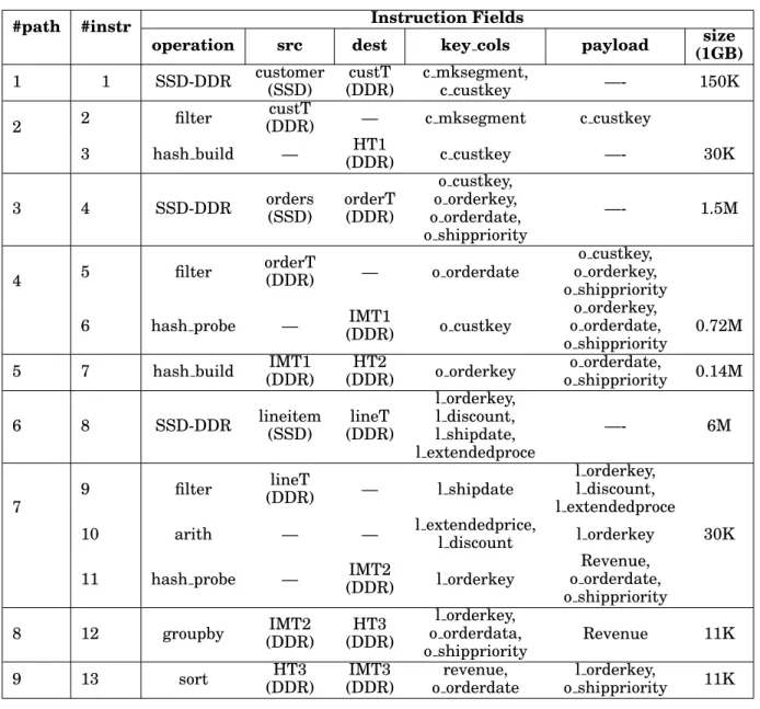
Due to explained query plan of Q03, the required instruction set of AxleDB to process the given query is summarized in Table II. They are composed of many parameters, e.g., the operation (that defines the appropriate operation), the source (to determine the source of the data and corresponding address), the destination (to determine the destination of the data and the corresponding address), the key columns (the columns that are used as key during the query execution) and the payload (the columns that are only carried along). In summary, these instructions are used to establish the required data streaming paths in AxleDB to process the example query Q03, by following the query plan in Figure 3. Accordingly, as an example, in Section 3.3 we illustrate how these instructions are used to establish one of the sample data streaming paths, #7, by following the process in Figure 2.

3.3. Establishing a Data Streaming Path: Elaboration for a Sample Data Path

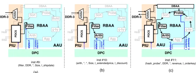
In this section, we explain how components of AxleDB are leveraged to process the ex-ample query. As it can be seen in Table II, the processing of Q03 can be accomplished by 13 AxleDB instructions that lead to creating 9 distinct data streaming paths. Among them, and as an example, we explain the required steps to create the sample data streaming path #7, which is depicted in Figure 4. As it can be seen, to establish the given data path #7, 3 QEI are used (#9, #10, and #11). Each QEI determines a specific part of the data path #7 and finally, by the last instruction the path is established. Due to each instruction, the DPC generates the necessary control signals to the PIU, to set up the data movement path, and to the AAU, to activate and configure the required hardware accelerators. Accordingly, to establish the given data path, steps as below are proceeded:

(1) Instruction #9:As it can be seen in Figure 4(a), instruction #9 defines a filtering operation for the data in the DDR-3. Thus, the required actions arei)configuring the PDCS to stream in the data from the DDR-3, in this case lineT, to the AAU-RBAA. For this aim, the appropriate ports of the PDCS are utilized. And,ii) acti-vating the corresponding hardware accelerator, in this case filter unit, by setting it to work in theactivestate (state=1). Also, the query-specific filtering parameters are defined by DPC, ”l shipdate>1995-03-10”.

(2) Instruction #10:As it can be seen in Figure 4(b), instruction #10 defines an arith-metic operation for the filtered data. Thus, the only required action is to activate the arithmetic accelerator by setting it to work in theactivestate (state=1). Also, the convenient parameters of the arithmetic unit need to be set. For this aim, the DPC generates the required control signals to carry out the corresponding arith-metic operation, ”l extendedprice*(1-l discount)”. It is worth noting that for this instruction, as it does not have any valid source or destination parameters, we do not need to modify the PDCS configuration.

Table II: AxleDB instructions to process the example query, according to the query plan in Figure 3 (some of the fields such accelerator-specific parameters are omitted in this table.) The size column shows the size of the data stream for each data path, in terms of the number of rows, in 1 GB scale dataset.

#path #instr Instruction Fields

operation src dest key cols payload size (1GB)

1 1 SSD-DDR customer_{(SSD) (DDR)}custT c mksegment,_{c custkey} —- 150K

2 2 filter custT (DDR) — c mksegment c custkey 3 hash build — HT1 (DDR) c custkey —- 30K 3 4 SSD-DDR orders (SSD) orderT (DDR) o custkey, o orderkey, o orderdate, o shippriority —- 1.5M 4 5 filter orderT (DDR) — o orderdate o custkey, o orderkey, o shippriority

6 hash probe — _(DDR)IMT1 o custkey

o orderkey, o orderdate, o shippriority

0.72M

5 7 hash build IMT1

(DDR) HT2 (DDR) o orderkey o orderdate, o shippriority 0.14M 6 8 SSD-DDR lineitem (SSD) lineT (DDR) l orderkey, l discount, l shipdate, l extendedproce —- 6M 7 9 filter lineT (DDR) — l shipdate l orderkey, l discount, l extendedproce 10 arith — — l extendedprice, l discount l orderkey 30K

11 hash probe — IMT2

(DDR) l orderkey Revenue, o orderdate, o shippriority 8 12 groupby _(DDR)IMT2 _(DDR)HT3 l orderkey, o orderdata, o shippriority Revenue 11K 9 13 sort HT3 (DDR) IMT3 (DDR) revenue, o orderdate l orderkey, o shippriority 11K

(3) Instruction #11:As it can be seen in Figure 4(c), instruction #11 completes the es-tablishing of the data path #7, as it needs to write data into one of the data sources, DDR-3. Thus, data streaming will be started after this final step. Instruction #11 requires utilizing the hash probe accelerator by setting its state toactive(state=1). Consequently, the other accelerators in the AAU including aggregation, group by, hash build, and sort units are configured to work in thesilentstate to only pass the incoming stream of data to the next unit in the RBAA. Also, the hash probe key, in

Fig. 4: Establishing the data streaming path #7 by composing together different AxleDB instructions #9, #10, and #11. The detailed connections between DPC, AAU, and PIU are shown. Among them, the highlighted components/connections represent the corresponding parts that are utilized by each AxleDB instruction to set up the given data streaming path. The control signals for the PIU and the AAU are gener-ated by DPC.

this casel orderkey, is determined by the DPC. The hash probe unit needs another DDR-3 memory access to read the hash table, in this case HT2. For this aim, the corresponding port of the DBAA is activated to access the hash table from DDR-3. In summary, the data streaming path #7 leads toi)read the lineT table from DDR-3, ii)filter the incoming data stream based onl shipdate item,iii)apply an arithmetic function for the filtered data,iv)probe the stream of the data based on thel orderkey

in the HT2 hash table., and finally, v) write the probed data into the DDR-3 in the index IMT2. In total, there are 3 distinct DDR-3 data access paths in this data path, i.e., i)to stream in the input data (as explained above in the part of instruction #9) through RBAA,ii)to access the hash table in the hash probe unit (as explained above in the part of instruction #11) through a direct DBAA bus, and finally,iii)to stream out the result data (as explained above in the part of instruction #11) through RBAA. As mentioned in Section 2, to manage the concurrent DDR-3 requests and optimally share its bandwidth, the arbiter in the PIU is exploited, which allows the priority to the DBAA requests to quickly serve the hash table accesses.

4. QUERY PROCESSING ACCELERATORS

In this section, we go through the architecture of the proposed accelerators that are im-plemented to perform efficient query processing in AxleDB. We proposed query execu-tion units including filtering, arithmetic, aggregaexecu-tion, sorting, hash join, and groupby, as well as the MinMax indexing mechanism for I/O optimization.4

For developing, leveraging HLS tools, we have designed the filtering and aggrega-tion accelerators in Vivado HLS [15], where we have been able to exploit the data parallelism via Vivados compiler directives. For task-parallel and control-oriented ac-celerators, such as the hash join and sort engines, Bluespec SystemVerilog [16] is used. 4_{In the rest of the paper, we assumed input data table as a set of tuples, pairs ofkeyandvalue.keyrefers to} the column(s) of data, used for performing the main query operation, e.g., sorting key in a sorter unit.Value refers to the other columns that need to be carried to make the final resulting data.

Verilog RTL code is employed for the integration of interface controllers. We select to employ these HLS tools as a result of our previous empirical analysis of a representa-tive set of HLS tools for database acceleration [17].

4.1. Filtering Operations, Arithmetic, and Logic Unit

Database filtering is relational operations that test the numerical or logical relations between columns, in the form of numerical and/or Boolean values. The key importance of filtering operations in an SQL query is to reduce the amount of data for further processing [18], [19]. For this purpose, we designed a compile-time parameterizable, variable width, n-way compute engine that takes in rows of data as inputs, applies a filtering operation to the desired fields and produces an output bitmap. This bitmap de-termines the resulting rows for further processing. Similarly, we designed arithmetic, and logical compute engines. The arithmetic engine supports the integer Add, Sub, and Mult operations5_{, whereas the logical engine supports the NOT, AND, OR, NOR and} NAND operations. Also, keywords such as IN, SOME, and EXISTS can also be mapped to multiple logical operations. The design behind the filtering, arithmetic and logical blocks encapsulates three major decisions:

– Width ofkey:In this work, we explored 32-bit and 64-bit data widths for filtering, arithmetic, and logical operations. There are no limitations regarding custom data width selection; since Vivado HLS supports it. Nevertheless, using larger data widths means utilizing more LUT resources. This becomes specifically critical for low-cost FPGAs because they include LUTs with fewer inputs. Overprovisioning data widths can result in area utilization problems and decreased computational power by failing to meet the timing constraints.

– Number of parallel units: The number of units determine how much data-parallelism can be supported. For this purpose, the approach we followed is to de-termine the data widths according to the width of DDR-3 RAM line. Thus multiple blocks can process a memory line that is composed of multiple elements of data. In this work, one line of DDR-3 RAM is 512-bits and data widths could be either 32 or 64-bits. Thus, 512/32 =16 or 512/64 = 8 units are instantiated in parallel. It is worth noting that in the TPC-H benchmarks that we looked into, we havent hit to the cases where the required data width is more than 512 bits. Since the 512-bit data width is a property of the DDR-3 interface itself, for more data width, the requirements would be to either (i) use a newer/different technology (High Bandwidth Memory(HBM), 3D stacking, hybrid memory cube, etc.) that supports a wider memory interface, or to (ii) lay the data out in parallel DDR-3 channels. In either case, the AxleDB architecture does not have any inherent limitations regarding the bandwidth to memory.

– Pipelining:We designed all supported filtering, arithmetic and logical operations of AxleDB to be fully pipelined, with an initiation interval of 1 cycle. Thus, all query plans that allow pipelining can be fully supported by our filtering, arithmetic logical and aggregation blocks.

For a given filtering, arithmetic or logical operation, each input data can either be compared with another input data from another table, or it can be compared with a constant. For this purpose, scratchpad registers (SPR) are utilized. These registers hold values and allow the aforementioned operators to be applied to the input data and the SPRs. Our filter unit is capable of performing numerous logical operations, including the BETWEEN operator. As an example, in Figure 5(a), the input data array 5_{The DIV operator (for floating point) can be configured to be included in the AxleDB architecture, it is quick} to implement it using Vivado HLS, but it requires a large area and latency. Since we only needed to use this operator only a single time in Q14, we decided not the include the hardware for this operator, and to perform this operation in software (on the host) instead.

Fig. 5: (a) Filtering blocks that apply the BETWEEN operation to input data using scratch-pad registers (b) SUM aggregation using binary fan-in technique.

holds the column values that require filtering. SPR 0 and SPR 1 hold the filtering qualifiers, the values that input data must be compared against. Thus, input data and SPRs are forwarded to the filters and output are generated. For instance, to perform date 1996-01-11 <l shipdate <date 1995-01-11 BETWEEN operation, SPR 0 holds date 1995-01-10 and SPR 1 holds date1996-01-12 in 32-bit POSIX time format. For other operations, SPRs work the same way.

4.2. Aggregation Unit

Aggregation operations reduce an input set to a single value. In AxleDB, we provide an n-way aggregator engine that supports MAX, MIN, COUNT, SUM and AVERAGE. Aggregation units are designed with the same three design decisions in mind, which were explained in Section 4.1. They are also fully pipelined with an initiation interval of 1 clock cycle. Similar to the filtering unit, aggregation units are designed to take columns as inputs and to finally combine the results to calculate the final aggregate value. All aggregation operations are implemented in Vivado HLS using the binary fan-in technique. Based on the input array, the size n binary fan-in depth is log2n, and n-1 operators are necessary to form the operator tree. An example is presented in Figure 5(b), where for 8 input elements, 7 sum operators are instantiated to generate a single pipelined result.

Multiple filtering/aggregation blocks can be exploited in two ways: pipelining or time-multiplexing. In a pipelined design, streaming data through multiple instances of the accelerators achieve multiple operations in a single pass. However, for area ef-ficient designs, a single accelerator can be used in a time-multiplexed way. For the studied benchmarks, instantiating multiple filter/aggregation blocks in a pipeline pro-vides the maximum throughput, as we further detail in Section 6.1.

4.3. Hash-Based Units: Table Join and GroupBy

For table joins and groupby operations, we proposed an efficient hashing-based engine. As a first step for table joins, a hash table is constructed using a hash function over the key(Build phase). Later on, once constructed, the entries of the second table are probed against this hash table to generate the resulting joint table (Probe phase). For the groupby operation, building a hash table over the key can already result in the desired output data.

Hash collisions are critical in hash-based table join and groupby operations because they can be detrimental to good performance. Hash collisions indicate a situation where different keys refer to the same index of the hash table. To resolve collisions, software fallback [6] is a promising solution, but it causes extra overheads. Alterna-tively, collisions can be managed in hardware as well, by chaining the colliding hash

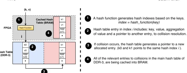
Fig. 6: Hash table caching for enhanced acceleration of table join and groupby. The DDR-3 that locates the hash table is partitioned into two parts. The first part is in-dexed and uncached and the second part is only used for collisions and is cached inside the FPGA. (k0andk1are the colliding keys).

table entries [20]. Such behavior can cause pointer chasing and undermine good per-formance, especially if the hash table is located in high latency DDR-3 memory. To alleviate this problem, thanks to the architecture of FPGAs, we proposed a pure hard-ware solution. In contrast, the previous techniques such as [6], whereas only off-chip memory is exploited, we targeted to cover the high latency of DDR-3 RAM by exploiting the low-latency Block RAM resources of the FPGA. However, since the size of BRAMs is not large enough to cope with entire hash tables, we present a hash table caching mechanism. We presented an early version of the hash table caching technique in [21]. The cache in BRAM includes some of the hash tables entries that were recently used. Faster access to the cached entries provides a more streamlined execution. Conse-quently, utilizing DDR-3 RAM and Block RAMs enables us to both,(i)to use the full capacity of the DDR-3 RAM to store entire large hash tables,(ii)and to exploit Block RAMs as a hash cache.

As it can be seen in Figure 6, the main components of the proposed engine area Lin-ear Feedback Shift Register(LFSR)-based hash function that allows constant pipelin-ing, Block-RAMs of FPGA as the cache, and the logic of the table join/groupby mech-anism. We can store values (for table join), or an aggregation of values (for groupby) inside the hash table, in conjunction with thekeyand a pointer to another hash tables entry for collision resolution. This way, exploiting Block RAM resources, the cache is used to avoid slow pointer chasing effectively. It contains direct-mapped copies of hash tables entries that are recently accessed after a collision. We used the Least Significant Bit (LSB) of the hash index as the index to the cache entry, and the Most Significant Bit (MSB) as a cache tag to discard false positives of cache accesses. The proposed mechanism could also work in conjunction with the multi-threaded hash join engines [22]. The performance of our caching technique is evaluated in Section 6.1.2.

For any hash collision, in the worst case, we need to perform an additional memory read to access the corresponding hash table entry in the chain, which incur an 8-16 clock cycles latency. This is the average latency of the memory part in our platform. However, in the best case, when the read operation of the hash table entry is hit in the cache, (in BRAM) only one cycle is enough to access it.

Fig. 7: The architecture of sort engine in AxleDB. (a) Spatial sorter. (b) merge-sort tree. By the way, the hardware-software co-designed bloom-filter-based hash join acceler-ator is proposed in [23] that can be a complementary solution for the introduced hash table caching technique in this paper. We do not use several hash functions, and we do not run into false positive problems as with the Bloom filter approach. In contrast, we utilize almost most of the free BRAMs of the FPGA as a cache to achieve an improved throughput. In [23], as Bloom filters use BRAMs to store the bit vector, the processing of large data tables may be limited by the size of BRAMs.

4.4. Sorting and Merging Unit

To efficiently sort large datasets, we used two hardware structures in AxleDB.(i)The sorter is an extension of the spatial sorter [24], which allows AxleDB to effectively support the LIMIT operation. Furthermore,(ii)we implemented a merge-sort tree to merge partially sorted sets to be able to sort large input sets.

4.4.1. Spatial Sorter.A spatial sorter is composed of a chained array of sorting regis-ters, each of which effectively performs a compare and swap operation. As it can be seen in Figure 7(a), each sorter node is made up of a comparator, two registers, and two multiplexers [25]. New elements are inserted at the beginning of the sorted array. At each clock cycle and on each node, an input value is compared with the current value. The larger value is stored in the sorter node, and the smaller value is passed on to the next node. An n-node spatial sorter has a time cost of 2n cycles to sort an input set of size n. For this, for n cycles, n tuples are pushed in one by one at the head of the sorter. Later on, in cycle n, a flush signal is pushed in at the head node. Until cycle 2n, this signal propagates until the end of the sorting pipeline. Meanwhile, the tuples that last entered are shifted deeper in the pipeline until they find their correct final positions. By 2n cycles, all the tuples that reside in the nodes of the pipeline are sorted. Then it is possible to start pushing out and writing back the resulting set, and at the same time, to begin receiving a new unsorted input set. The resource usage of the spatial sorter is proportional to its number of inputs. For our case where we want to support wide data inputs, the spatial sorter is a resource-friendly solution.

4.4.2. Merging Sorted Sets.To merge-sort input sets that are larger than the sorter size, the sorter was coupled with a merging tree, as shown in Figure 7(b). N-way input

buffers feed the merger with sorted sets. At each cycle, the smaller input data passes through on all nodes, therefore in the lowest node, the smallest data is output. Block RAMs of FPGA were used as input buffers to sustain constant throughput under DDR-3 RAM latency.

4.4.3. Sorting with the LIMIT Operation.An inherent advantage of employing a spatial sorter is the LIMIT operation. The LIMIT operation is very commonly used in database analytics. We profit from this fact to have a sorter that can do the LIMIT operation at O(n) complexity. However, the best property of this kind of sorting hardware is that it is very regular, chaining-friendly, and maps very well on the FPGA fabric. The LIMIT operation returns only the top n elements of a sorted set. The spatial sorter of sizen, when constantly fed with input tuples each cycle (regardless of its size), essentially acts as a LIMITnoperation.

After passing the whole input set through the sorter pipeline, the flush signal will return the sorted top n elements of the set. Therefore, on AxleDB, sorting with a LIMIT operation (wheren<sorter nodes) has a linear time cost ofncycles and furthermore does not require a merging operation afterward. We need to ensure that in a LIMIT

noperation, then results fit inside the sorter nodes, and do not overflow. In the case of overflow, a complete sort (that also uses the merge tree) would be needed. Later in Section 6.1.3, we demonstrate this operation, working with query Q03.

4.5. Block-Level MinMax DataBase Indexing Unit

Database indexing is a technique that improves the speed of retrieving the database tables and is widely used in software DBMS [26], [27], [28]. Indexes are meta-data of the original dataset that are used to locate data quickly. Although there is no standard for generating database indexes, the most commonly used types are B-Tree, Bitmap, and MinMax [28]. In this paper, we focused on the MinMax indexing technique, be-cause it has a straightforward and efficient idea behind, and in addition, it does not suffer from the usual overheads of the other indexing methods, i.e., the large size of in-dexes in B-Tree method6_{, or the low utilization of Bitmap indexing for high-cardinality} data method. Some of the software DBMS are already equipped with this technique in different naming: BRIN (Block Range Indexes) in PostgreSQL [29] or Storage Indexes in Oracle [30]. On the other hand, although database indexing is supported in one of IBMs FPGA-coupled products, Netezza [31] which is called zone maps, to the best of our knowledge, it is not investigated thoroughly in FPGA research community yet.

MinMax indexing is an access method intended for the fast scanning of data tables in SSD, by avoiding accesses to the unneeded blocks. We propose a block-level version that uses min and max (bM in,bM ax) values for each data block. As a pre-step of query

processing, the aim is to determine data blocks that according to their index values, will or will not pass the filter. This way, the aim is to avoid retrieving those unnecessary blocks from SSD.

In AxleDB, in database creation time, the index values are generated and stored on the SSD. Thus, SSD is partitioned into two distinct parts: data blocks including data tables, and index blocks including index values. The supported filtering operations are LESS THAN (<), MORE THAN (>) and BETWEEN (<>). The functionality of the index checking unit is shown in Listing 1, for a single blocki. Depending on the filtering operator, only and if only these conditions are satisfied, it would be necessary

6_{In Section 6.2, we reported some experimental results from PostgreSQL equipped with B-Tree indexing.} We observed that in some queries, the I/O transmission of indexes dominates the original dataset execution, causing significant performance degradation.

to retrieve the block i from SSD. (biM in and biM ax are the min, max index values of

data blocki.qM in andqM axare the filtering qualifiers.)

Listing 1: The functionality of index checking function for a sample blocki.

O P E R A T I O N I n d e x C h e c k i n g F u n c t i o n L E S S T H A N ( Field <qM ax) (qM ax>=biM in)

M O R E T H A N ( Field >qM in) (qM in<=biM ax)

B E T W E E N (qM ax< Field <qM in) (qM ax>=biM in) &&(qM in<=biM ax)

The index checking function is repeated for all of the indexes, thus, finally we ob-tain the list of only the necessary blocks of data. Although the total size of indexes is proportional to the number of data blocks (size of total data divided by block size), as we only store two values for each block (bM in,bM ax), the size of index storage is mainly

negligible, leading to a small performance overhead. We exploited local Block RAMs of the FPGA to store indexes. The following steps summarize running AxleDB with MinMax indexing capability, as a pre-step of query processing:

(1) AxleDB initializes the index checking unit with one of the supported operations (<,>,<>) and their qualifiers (qM in,qM ax).

(2) AxleDB first retrieves the index blocks from SSD. Later on, for each particular index that corresponds to a particular data block, AxleDB checks it (as shown in Listing 1). Accordingly, the list of the required data blocks for the further process-ing are generated in the Block RAMs.

(3) Once the index checking process is completed, AxleDB continues the query process-ing by retrievprocess-ing only those necessary data blocks that are listed in Block RAMs. The efficiency of MinMax indexing technique highly depends on the data distribution model. For instance using this technique, for the highly ordered dataset, most of the unnecessary data blocks can be detected, which in turn leads to a significant reduction in I/O transmission. We further analyze it in Section 6.1.4.

5. EVALUATION METHODOLOGY 5.1. Configuration of the AxleDB

We developed AxleDB on a VC709 FPGA development board with an XC7VX690T FPGA and 4GB of DDR-3 RAM. It accesses a Crucial M4-256GB SSD through a cus-tomized version of an SATA-3 controller, based on Groundhog [12]. We used a relatively large block size (512 KB), which can help minimize the SSD overheads and, thus lead to significant improvements in data transfer throughput. AxleDB is directly attached to the host through a high-speed PCIe-3 interface for data/instruction transmission. Our accelerators and DDR-3 RAM controllers run at 200 MHz, PCIe-3 controller at 250 MHz, and SATA-3 at 150 MHz, therefore we used various synchronizing FIFOs for clock domain crossing.

In order to thoroughly evaluate the efficiency of the various components of AxleDB, we ran the benchmarks in two modes:(i)cold run, where the input datasets are orig-inally located inside the SSD, and(ii)warm run, without considering the I/O time of SSD, and assuming that the datasets are already loaded in the DDR-3 memory of the platform. Thus, in the warm mode, the total processing time of the queries does not in-clude the time of loading input data tables from SSD to the DDR-3. To better analyze the cold and warm runs, we partitioned the total execution time of the query into three parts:(i)the I/O time of SSD, i.e. the required time of transferring input datasets from the SSD to DDR-3 memory of AxleDB,(ii)execution time, i.e. the query execution time of the processing units (accelerators) of AxleDB, and(iii)the time spent on the other

parts, including query planning time7_{, the time for PCIe-3 data transfers, and finally} the overhead of device controllers. The last portion is negligible for large scales of data. 5.2. Configuration of Comparison Cases: MonetDB, PostgreSQL and CStore

We evaluated AxleDB against the query processing engines of several state-of-the-art software DBMS:(i)MonetDB 11.21 [9] as a popular column-oriented database system, (ii)PostgreSQL 9.5 (PGSQL) as a popular object-relational row-oriented database sys-tem [8], and (iii)CStore as the PostgreSQL’s column-oriented data store extension [10]. More specifically, it is worth noting that:

—MonetDBhas several unique features to optimize the I/O and computation, simul-taneously:(i)it is built on a column representation of database relations,(ii)it has an innovative storage model based on vertical fragmentation,(iii) it has a CPU-tuned query processing architecture,(iv)it exclusively tries to use the main mem-ory for the processing, and(v) it has the capability of running queries in a multi-threaded fashion.

—PostgreSQLis intrinsically a row-oriented database system. It is equipped with a wide set of database indexing methods, such as BRIN, B-Tree, etc., that can be used as an appropriate comparison case with the proposed FPGA-based MinMax index-ing technique in AxleDB. Also, to get better performance, PostgreSQL is extended with an extra patch to support fixed-decimal data type [33]. Fixed decimal is a fixed precision decimal type which provides a subset of the features of PostgreSQL’s built-in NUMERIC type, but with built-increased performance.

—CStoreis an extension that enables column-oriented data storage in PostgreSQL. It uses the Optimized Row Columnar (ORC) format, which brings some benefits such as; compression, column-projection, and skips indexes (similar to MinMax/BRIN). We run MonetDB, PostgreSQL, and CStore on a Supermicro server machine, equipped with two E2630 Intel Xeon processors, with a total of 12 cores and 24 threads, running at a maximum frequency of 2.3 GHz. The server is attached to a Crucial M4 SSD disk (as in the AxleDB) to store database tables. The operating system (OS) is Ubuntu 64-bit 12.04, with kernel version 3.13. To have a fair comparison, we equip the server with the same size of the memory with AxleDB, 4GB DDR-3. However, we observe a system crashes of the PostgreSQL/CStore runs for the 10GB scale bench-marks, which is the consequence of the insufficient system memory. Thus, for this spe-cial case, the server is equipped with a larger capacity of memory. We observed that at least 16 GB is enough to accomplish the query processing without system crash-ing. Consequently, in summary, the host is equipped with 4GB and 16GB for Mon-etDB and PostgreSQL/CStore experiments, respectively. Furthermore, similar to the AxleDB, software DBMS experiments were also ran in two modes,i)cold mode, where input data tables are located in the SSD, andii)warm mode, where input data tables are already loaded into the DDR-3 memory from the original database storage, SSD. To obtain their execution times, we ran each query twice, consecutively. The first run is in the cold mode. In contrast, the second run is executed using internal buffers, where the data is already located inside the main memory of the server. The second run is in the warm mode.

7_{As the query planning of AxleDB is currently a manual process, thus to have a fair comparison with} software DBMS, we extracted the average time of the query planner of MonetDB (8ms for cold and 2ms for warm runs), and used it in this part [32].