Software implementation and testing of GARCH models

(1)

Software implementation and testing

of GARCH models

G F LEVY

NAG Ltd, Wilkinson House,

Jordan Hill Road,

Oxford, OX2 8DR, U.K.

(email: [email protected])

(2)

Abstract:

This paper describes the software implementation of GARCH routines in Fortran 77.

The routines considered here cover both symmetric and asymmetric GARCH and also shocks

having Gaussian and non-Gaussian distributions. Extensive examples of using the software are

provided and the test results from Monte Carlo simulations are presented.

Keywords:

GARCH, ARCH, maximum likelihood estimation, volatility, generalised

autoregressive heteroskedasticity, asymmetry, Fortran 77

1 Introduction

The modelling of sequences with time-dependent variance is crucial to many areas of

mathematical finance. This technical report describes the software implementation and testing of

a set of univariate generalised autoregressive conditional heteroskedastic (GARCH) routines

that have been developed at NAG Ltd for its numerical libraries. Although we are primarily

concerned with GARCH software that has been developed for the next release of the NAG

Fortran 77 Library [1], some GARCH software is already contained in the current version of the

NAG C Library [2]. The Fortran 77 software described here can be used for GARCH(

p,q

) models

with arbitrary values of

p

and

q

. There are routines for the generation of GARCH sequences,

model estimation and volatility forecasting. The estimation routines return not only the parameter

estimates but also other important statistics such as: the standard errors, the scores and the

value of the log-likelihood function for the calculated model parameters.

Other capabilities of the software include the following:

•

regression-GARCH(

p,q

) models

•

symmetric models

•

asymmetric models

•

shocks with Gaussian and non-Gaussian distributions

Since both the NAG Fortran 77 and C libraries are implemented as Dynamic Link Libraries (DLLs)

the GARCH software can be easily used from the Microsoft Windows environment. This means

that the GARCH routines can be readily incorporated into Microsoft software such as Excel, Visual

Basic, etc.

2 The GARCH models

The standard (symmetric) regression-GARCH(

p,q

) model [3] [4] [5], with Gaussian shocks

ε

_t

,

takes the following form:

∑

= − − = −

+

=

+

=

p j j t i t q i i t t t t t T t t

h

N

b

x

b

y

1 2 1 1 0 1 0

,

|

(

0

,

)

β

ε

α

ψ

ε

This process is described by

q

+ 1 coefficients

,

i

0

,

q

,

i

=

K

α

p

coefficients

β

i

,

i

=

1

,

K

,

p

,

mean

,

0

b

k

linear regression coefficients

b

i

,

i

=

1

,

K

,

k

,

endogenous/exogenous variables

y

_t

and

x

_t

(3)

It should be noted that for

p

= 0 a GARCH(

p,q

) model is also called an ARCH(

q

) model.

Empirical studies on financial time series have shown that they are characterised by increased

conditional variance

h

_t

following negative shocks (bad news). The distribution of the shocks have

been also found to exhibit considerable leptokurtosis. Since the standard Gaussian GARCH model

cannot capture these effects various GARCH model extensions have been developed [6].

The asymmetric GARCH models considered here are:

AGARCH(

p,q

)-type1

∑

= − − =

+

=

p j j t i i t q i i t

h

1 2 1 0

α

(

ε

γ

)

β

α

AGARCH(

p,q

)-type2

∑

= − − − =

+

=

p j j t i i t i t q i i t

h

1 2 1 0

α

(|

ε

|

γε

)

β

α

GJR-GARCH(

p,q

), or Glosten, Jagannathan and Runkle GARCH [7]

∑

= − − − =

+

=

p j j t i i t t q i i t

S

h

1 2 1 1 0

(

α

γ

)

ε

β

α

where

S

_t

=

1

if

ε

_t

<

0

and

S

_t

=

0

if

ε

_t

≥

0

EGARCH(

p,q

), or exponential GARCH

[

]

(

|

E

|

z

|

)

ln(

)

ln(

1 1 i -t 1 0

∑

= − = − − =

+

−

+

=

p j j t i q i i t i i t q i i t

z

h

α

φ

β

where

t t t

h

z

=

ε

and

E

[

|

z

t−i

|

]

denotes the expected value of

|

z

t−i

|

In all these models the shocks

,

ε

_t

,

can either have a Gaussian distribution or Student's

t

-distribution with a specified number of degrees of freedom.

In AGARCH-type1 the asymmetric effects are modelled via the extra parameter

γ

.

For example,

in the standard GARCH(1,1) model when

h

t−1

is fixed

h

t

=

h

(

ε

t−1

)

is a parabola with a minimum

at

ε

_t₋₁

=

0

.

The introduction of the additional parameter

γ

shifts the parabola horizontally so that

the minimum occurs at

ε

_t₋₁

=

−

γ

.

The conditional

variance following negative shocks can

therefore be enhanced by choosing

γ

<

0

,

so that

h

(

−

ε

_t₋₁

)

>

h

(

ε

_t₋₁

)

for

ε

_t₋₁

>

0

.

In an AGARCH-type2 model the inclusion of

γ

can also result in an enhancement of

h

t

following

a negative shock

ε

_t₋₁

.

For a GARCH(1,1) model

h

(

−

ε

_t₋₁

)

>

h

(

ε

_t₋₁

)

for

ε

_t₋₁

>

0

and

γ

<

0

.

Similarly in the GJR-GARCH(1,1) model the value of

h

t

is increased above the symmetric case

when

ε

_t₋₁

<

0

and

γ

>

0

.

(4)

For EGARCH, asymmetric response arises from the terms

_t _i q i i

z

− =

∑

1

α

.

In an EGARCH(1,1), if

0

1

<

α

then a negative shock

ε

_t₋₁

<

0

increases the value of

h

_t

,

that is

ln

{

h

(

−

z

_t₋₁

)

} {

>

ln

h

(

z

_t₋₁

)

}

.

All the GARCH processes above are uniquely described by the parameter vector

θ

, where

,

)

,

(

b

₀

b

T

ω

T

θ

=

ω

T

=

(

α

₀

,

α

₁

,

α

₂

,

K

,

α

_q

,

β

₁

,

β

₂

,

K

,

β

_p

,

γ

)

and

b

T

=

(

b

₁

,

K

,

b

_k

)

.

The GARCH model implementations here all rely on finding the value of

θ

which maximises the

conditional log-likelihood (objective) function

where

T

is the number of terms in the sequence.

This is achieved by starting with an initial approximation

for

θ

and then using numerical

optimisation to iterate to an acceptable solution. In all the GARCH estimation routines, apart

from EGARCH, an analytic expression for the Jacobian of the objective function was used for

the optimisation stage.

The standard errors for the parameter estimates can be computed by using the well known

result [8] that the maximum likelihood estimate for

θ

is asymptotically normal with mean

θ

and covariance matrix

ℑ

−1

where

ℑ

(The Fisher Information Matrix)

is given by:

3 The GARCH software

Here we list the available software for sequence generation, model parameter estimation, and

forecasting of regression-GARCH(

p,q

) sequences.

3.1 Generation

The following routines generate a given number of terms from various symmetric and

asymmetric GARCH(

p,q

) sequences.

Specification

AGARCH-type1

SUBROUTINE G05HKF (DIST, NUM, IP, IQ, THETA, GAMMA, DF, HT, YT, FCALL, RVEC, IFLAG)













∂

=

ℑ

∑

= T i T

lf

1 2

E

θ

∑

=









+

=

T i i i i

h

lf

1 2

)

(

log

2

1

ε

(5)

AGARCH-type2

SUBROUTINE G05HLF (DIST, NUM, IP, IQ, THETA, GAMMA, DF, HT, YT, FCALL, RVEC, IFLAG)

GJR-GARCH

SUBROUTINE G05HMF (DIST, NUM, IP, IQ, THETA, GAMMA, DF, HT, YT, FCALL, RVEC,IFLAG)

EGARCH

SUBROUTINE G05HNF (DIST, NUM, IP, IQ, THETA, DF, HT, YT, FCALL, RVEC, IFLAG)

The routine parameters have the following meanings:

Parameters

DIST - CHARACTER*1.

On entry, the type of distribution to use for

ε

_i if DIST = 'N' then a Normal distribution is used. if DIST = 'T' then a Student's t-distribution is used.

NUM - INTEGER

On entry, the number of terms in the sequence, T IP - INTEGER.

On entry, the number of moving average coefficients, p IQ - INTEGER.

On entry, the number of auto-regressive coefficients, q THETA- DOUBLE PRECISION array.

On entry, the parameters of the GARCH model

GAMMA - DOUBLE PRECISION.

On entry, the asymmetry parameter

γ

for the GARCH sequence.

DF - DOUBLE PRECISION

On entry, the number of degrees of freedom for the Student's t-distribution. It is not referenced if DIST = 'N'

HT - DOUBLE PRECISION array.

On exit, the conditional variances for the GARCH sequence, h_i,i=1,K,T

YT - DOUBLE PRECISION array.

On exit, the observations for the GARCH sequence,ε_i,i=1,K,T.

FCALL - LOGICAL.

On entry, if FCALL = .TRUE. then a new sequence is to be generated, else a given sequence is to be continued using the information in RVEC.

RVEC - DOUBLE PRECISION array.

On entry, the array contains information required to continue a sequence if FCALL = .FALSE. On exit, contains information that can be used in a subsequent call, with FCALL = .FALSE.

IFLAG - INTEGER. The error indicator

(6)

3.2 Estimation

The following routines estimate the model parameters of various symmetric and asymmetric

regression-GARCH(

p,q

) sequences.

Specification

AGARCH-type1

SUBROUTINE G13FAF (DIST, YT, X, LDX, NUM, IP, IQ, NREG, MN, ISYM, THETA, SE, SC, COVAR, LDC, HP, ETM, HTM, LGF, COPTS, MAXIT, TOL, WORK, LWORK, IFLAG)

AGARCH-type2

SUBROUTINE G13FCF (DIST, YT, X, LDX, NUM, IP, IQ, NREG, MN, THETA, SE, SC, COVAR, LDC, HP, ETM, HTM, LGF, COPTS, MAXIT, TOL, WORK, LWORK, IFLAG)

GJR-GARCH

SUBROUTINE G13FEF (DIST, YT, X, LDX, NUM, IP, IQ, NREG, MN, THETA, SE, SC, COVAR, LDC, HP, ETM, HTM, LGF, COPTS, MAXIT, TOL, WORK, LWORK, IFLAG)

EGARCH

SUBROUTINE G13FGF (DIST, YT, X, LDX, NUM, IP, IQ, NREG, MN, THETA, SE, SC, COVAR, LDC, HP, ETM, HTM, LGF, COPT, MAXIT, TOL, WORK, LWORK, IFLAG)

The routine parameters have the following meanings:

Parameters

DIST - CHARACTER*1

On entry, the type of distribution to use for

ε

_i

.

If DIST = 'N' then a Normal distribution is used, if DIST = 'T' then a Student's t- distribution is used.

YT - DOUBLE PRECISION array.

On entry, the sequence of observations, ε_i,i=1,K,T.

X - DOUBLE PRECISION array.

On entry, the

i

th

row of X contains the time dependent exogenous vector, x_i,i=1,K,T.

LDX - INTEGER.

On entry, the first dimension of the array X NUM - INTEGER.

On entry, the number of terms in the sequence, T

IP - INTEGER.

On entry, the number of auto-regressive coefficients, q NREG - INTEGER.

On entry, the number of regression coefficients, k MN - INTEGER.

On entry, if MN = 1 then the mean term

b

₀ will be included in the model

ISYM - INTEGER.

On entry, if ISYM = 1 then the asymmetry term

γ

will be included in the model (this only applies to G13FAF)

(7)

On entry, the initial parameter estimates for the vector

θ

On exit, the estimated values

θ

ˆ

for the vector

θ

SE - DOUBLE PRECISION array. On exit, the standard errors for

θ

ˆ

SC - DOUBLE PRECISION array. On exit, the scores for

θ

ˆ

COVAR - DOUBLE PRECISION array.

On exit, the covariance matrix of the parameter estimates

θ

ˆ

,

that is the inverse of the Fisher Information Matrix.

LDC - INTEGER.

On entry, the first dimension of the array COVAR HP - DOUBLE PRECISION

On entry, if COPTS(2) = .FALSE. then HP is the value to be used for the pre-observed of the conditional variance. If COPTS(1) = .TRUE. then HP is not referenced.

On exit, if COPTS(2) = .TRUE. then HP is the estimated value of the pre-observed of the conditional variance.

ET - DOUBLE PRECISION array.

On exit, the estimated residuals, ε_i,i=1,K,T.

On exit, the estimated conditional variances, h_i,i=1,K,T

LGF - DOUBLE PRECISION.

On exit, the value of the likelihood function at

θ

ˆ

COPTS - LOGICAL array

If COPTS(1) = .TRUE. then stationary conditions are enforced, otherwise they are not.

If COPTS(2) = .TRUE. then the routine provides initial parameter estimates of the regression terms, otherwise these are provided by the user.

MAXIT - INTEGER.

On entry, the maximum number of iterations to be used by the optimisation routine when estimating the GARCH parameters.

TOL - DOUBLE PRECISION

On entry, the tolerance to be used by the optimisation routine when estimating the GARCH parameters.

WORK - DOUBLE PRECISION array, workspace.

LWORK - INTEGER.

On entry, the size of the work array WORK.

IFLAG - INTEGER. The error indicator.

(8)

3.3 Forecasting

The following routines compute the volatility forecast for various symmetric and asymmetric

GARCH(

p,q

) sequences.

Specification

AGARCH-type1

SUBROUTINE G13FBF (NUM, NT, IP, IQ, THETA, GAMMA, CVAR, HT, ET, IFLAG)

AGARCH-type2

SUBROUTINE G13FDF (NUM, NT, IP, IQ, THETA, GAMMA, CVAR, HT, ET, IFLAG)

GJR-GARCH

SUBROUTINE G13FFF (NUM, NT, IP, IQ, THETA, GAMMA, CVAR, HT, ET, IFLAG)

EGARCH

SUBROUTINE G13FHF (NUM, NT, IP, IQ, THETA, CVAR, HT, ET, IFLAG)

The routine parameters have the following meanings:

Parameters

NUM - INTEGER.

On entry, the number of terms in the arrays HT and ET from the modelled sequence.

NT - INTEGER.

On entry, the forecast horizon,

χ

IP - INTEGER.

On entry, the number of auto-regressive coefficients, q THETA - DOUBLE PRECISION array.

On entry, model parameters of the GARCH sequence.

GAMMA - DOUBLE PRECISION.

On entry, the asymmetry parameter

γ

or the GARCH sequence.

CVAR - DOUBLE PRECISION array.

On exit, the forecast expected values of the conditional variance,

On entry, the sequence of past conditional variances for the GARCH(p, q) process, h_i,i=1,K,T.

ET - DOUBLE PRECISION array.

On entry, the sequence of past residuals for the GARCH(p, q) process, ε_i,i=1,K,T.

IFLAG - INTEGER. The error indicator.

(9)

4 Examples of usage

In this section we provide complete Fortran 77 source code to illustrate how the GARCH

routines can be used in practice. Each example generates a given type of GARCH sequence

models this using the appropriate GARCH estimation and then computes a volatility forecast. All

the examples consider GARCH sequences having both Gaussian and Student's

t

-distribution

shocks.

4.1 AGARCH-type1

In this example the following two models are considered:

•

An AARCH(3)-type1 model with shocks from a Gaussian distribution and observations,

y

t

=

b

0

+

ε

t

•

An AGARCH(1,2) -type2 model with shocks from a Student's

t

-distribution and

observations,

y

_t

=

b

+

x

_t

b

+

x

_t2

b

₂

+

ε

_t

1 1 0

Sequences of 1500 observations are generated for both of these processes, and then modelled

using initial parameter estimates of half the true values. The final model parameter estimates are

then output and a four step ahead volatility forecast is calculated.

Fortran source code

INTEGER NPARMX,NUM DOUBLE PRECISION ZERO

PARAMETER (NPARMX=10,NUM=1500,ZERO=0.0D0) INTEGER NUM1,NREGMX,MXNT,NT

PARAMETER (NUM1=3000,NREGMX=10,MXNT=400)

DOUBLE PRECISION FAC1,GAMMA,HP,LGF,MEAN,TOL,XTERM

INTEGER I,IFLAG,IP,IQ,ISYM,K,LDX,LWK,MAXIT,MN,NPAR,NREG,SEED LOGICAL FCALL

DOUBLE PRECISION BX(10),COVAR(NPARMX,NPARMX),ETM(NUM1), + HT(NUM1+10),HTM(NUM1),PARAM(NPARMX), + RVEC(40),SC(NPARMX),SE(NPARMX), THETA(NPARMX), + WK(NUM1*3+NPARMX+NREGMX*NUM1+20*20+1),X(NUM1,10), + YT(NUM1+10),CVAR(100) LOGICAL COPTS(2) CHARACTER*1 DIST DOUBLE PRECISION DF EXTERNAL E04UEF,G05HKF,G13FAF,G13FBF,G05CBF INTRINSIC ABS,DBLE,SIN

WRITE(*,*)'G13FAF Example Program Results' SEED = 111 NREG = 0 LDX = NUM1 BX(1) = 1.5D0 BX(2) = 2.5D0 BX(3) = 3.0D0 MEAN = 3.0D0 DO 5 I = 1,NUM FAC1 = DBLE(I)*0.01D0 X(I,1) = 0.01D0 + 0.7D0*SIN(FAC1) X(I,2) = 0.5D0 + FAC1*0.1D0 X(I,3) = 1.0D0 5 CONTINUE ISYM = 1 MN = 1 GAMMA = -0.4D0 IP = 0 IQ = 3 PARAM(1) = 0.8D0 PARAM(2) = 0.6D0 PARAM(3) = 0.2D0

(10)

PARAM(4) = 0.1D0 NPAR = 1 + IQ + IP LWK = NREGNUM+3NUM+NPAR+ISYM+MN+NREG+403 FCALL = .TRUE. IFLAG = 0 DIST = 'N' CALL G05CBF(SEED) CALL G05HKF(DIST,NUM,IP,IQ,PARAM,GAMMA,DF,HT,YT, + FCALL,RVEC,IFLAG) FCALL = .FALSE. CALL G05HKF(DIST,NUM,IP,IQ,PARAM,GAMMA,DF,HT,YT, + FCALL,RVEC,IFLAG) IFLAG = -1 DO 10 I = 1,NUM XTERM = ZERO DO 15 K = 1,NREG

XTERM = XTERM + X(I,K)*BX(K) 15 CONTINUE

IF (MN.EQ.1) THEN

YT(I) = MEAN + XTERM + YT(I) ELSE

YT(I) = XTERM + YT(I) END IF

10 CONTINUE

CALL E04UEF('Nolist')

CALL E04UEF('Print Level = 0') COPTS(1) = .TRUE. COPTS(2) = .TRUE. MAXIT = 200 TOL = 1.0D-16 DO 12 I = 1,NPAR THETA(I) = PARAM(I)*0.5D0 12 CONTINUE IF (ISYM.EQ.1) THEN THETA(NPAR+ISYM) = GAMMA*0.5D0 END IF IFLAG = 0 CALL G13FAF(DIST,YT,X,LDX,NUM,IP,IQ,NREG,MN,ISYM, + THETA,SE,SC,COVAR, + NPARMX,HP,ETM,HTM,LGF,COPTS,MAXIT,TOL,WK, + LWK,IFLAG) WRITE(*,*) WRITE(*,*)'Gaussian distribution' WRITE(*,*) WRITE(*,*)

+ 'Parameter estimates Standard errors Correct values'

DO 33 I = 1, NPAR WRITE(,'(F16.4,F18.4,F13.4)') THETA(I), + SE(I),PARAM(I) 33 CONTINUE IF (ISYM.EQ.1) THEN WRITE(,'(F16.4,F18.4,F13.4)') THETA(NPAR+1), + SE(NPAR+1),GAMMA END IF IF (MN.EQ.1) THEN WRITE(,'(F16.4,F18.4,F13.4)') THETA(NPAR+ISYM+1), + SE(NPAR+ISYM+1),MEAN END IF DO 34 I = 1, NREG WRITE(,'(F16.4,F18.4,F13.4)') THETA(NPAR+ISYM+MN+I), + SE(NPAR+ISYM+MN+I),BX(I) 34 CONTINUE NT = 4 CALL G13FBF(NUM,NT,IP,IQ,THETA,GAMMA,CVAR,HTM,ETM,IFLAG) WRITE (,)

WRITE (*,'(A,F12.4)') 'Volatility forecast = ',CVAR(NT) WRITE (*,*) DIST = 'T' NREG = 2 MN = 1 DF = 4.1D0 IP = 1 IQ = 2 ISYM = 1 GAMMA = -0.2D0 NPAR = IQ + IP + 1 LWK = NREG*NUM+3*NUM+NPAR+ISYM+MN+NREG+404

(11)

PARAM(1) = 0.1D0 PARAM(2) = 0.2D0 PARAM(3) = 0.3D0 PARAM(4) = 0.4D0 PARAM(5) = 0.1D0 FCALL = .TRUE. CALL G05CBF(SEED) CALL G05HKF(DIST,NUM,IP,IQ,PARAM,GAMMA,DF,HT,YT, + FCALL,RVEC,IFLAG) FCALL = .FALSE. CALL G05HKF(DIST,NUM,IP,IQ,PARAM,GAMMA,DF,HT,YT, + FCALL,RVEC,IFLAG) CALL G05HKF(DIST,NUM,IP,IQ,PARAM,GAMMA,DF,HT,YT, + FCALL,RVEC,IFLAG) IFLAG = -1 DO 110 I = 1,NUM XTERM = ZERO DO 115 K = 1,NREG

IF (MN.EQ.1) THEN

110 CONTINUE

CALL E04UEF('Print Level = 0') COPTS(1) = .TRUE. COPTS(2) = .TRUE. MAXIT = 200 TOL = 1.0D-16 DO 112 I = 1,NPAR THETA(I) = PARAM(I)*0.5D0 112 CONTINUE THETA(NPAR+ISYM) = GAMMA*0.5D0 THETA(NPAR+ISYM+1) = DF*0.5D0 CALL G13FAF(DIST,YT,X,LDX,NUM,IP,IQ,NREG,MN,ISYM, + THETA,SE,SC,COVAR,NPARMX,HP,ETM,HTM,LGF, + COPTS,MAXIT,TOL,WK,LWK,IFLAG) WRITE(*,*) WRITE(*,*)'Student t-distribution' WRITE(*,*) WRITE(*,*)

+ 'Parameter estimates Standard errors Correct values' DO 133 I = 1, NPAR WRITE(*,'(F16.4,F18.4,F13.4)') THETA(I), + SE(I),PARAM(I) 133 CONTINUE IF (ISYM.EQ.1) THEN WRITE(*,'(F16.4,F18.4,F13.4)') THETA(NPAR+ISYM), + SE(NPAR+ISYM),GAMMA END IF WRITE(*,'(F16.4,F18.4,F13.4)') THETA(NPAR+ISYM+1), + SE(NPAR+ISYM+1),DF IF (MN.EQ.1) THEN WRITE(*,'(F16.4,F18.4,F13.4)') THETA(NPAR+ISYM+1+MN), + SE(NPAR+ISYM+1+MN),MEAN END IF DO 134 I = 1, NREG WRITE(*,'(F16.4,F18.4,F13.4)') THETA(NPAR+ISYM+1+MN+I), + SE(NPAR+ISYM+1+MN+I),BX(I) 134 CONTINUE 199 CONTINUE NT = 4 CALL G13FBF(NUM,NT,IP,IQ,THETA,GAMMA,CVAR,HTM,ETM,IFLAG) WRITE (*,*)

WRITE (*,'(A,F12.4)') 'Volatility forecast = ',CVAR(NT) END

(12)

Output results

G13FAF Example Program Results

Gaussian distribution

Parameter estimates Standard errors Correct values 0.8031 0.0788 0.8000 0.6249 0.0570 0.6000 0.1803 0.0327 0.2000 0.0921 0.0237 0.1000 -0.5119 0.0682 -0.4000 2.9860 0.0324 3.0000 Volatility forecast = 2.8040 Student t-distribution

Parameter estimates Standard errors Correct values 0.0871 0.0230 0.1000 0.2174 0.0488 0.2000 0.2736 0.0820 0.3000 0.3588 0.0788 0.4000 -0.3240 0.0598 -0.2000 4.5173 0.5128 4.1000 3.0182 0.0431 3.0000 1.4727 0.0265 1.5000 2.4640 0.0302 2.5000 Volatility forecast = 0.4133

4.2 AGARCH-type2

•

An AGARCH(1,1)-type2 model with shocks from a Gaussian distribution and observations,

y

t

=

b

+

x

t

b

+

x

t

b

2

+

ε

t

2 1 1 0

•

An AGARCH(1,1)-type2 model with shocks from a Student's

t

-distribution and

observations,

y

_t

=

b

₀

+

x

1_t

b

₁

+

x

_t2

b

₂

+

ε

_t

Sequences of 1500 observations are generated for both of these processes, and then modelled

then output and a four step ahead volatility forecast is calculated.

Fortran source code

PARAMETER (NPARMX=10,NUM=1500,ZERO=0.0D0) INTEGER NUM1,MXNT,NREGMX,NT

PARAMETER (NUM1=3000,MXNT=400,NREGMX=10)

DOUBLE PRECISION FAC1,GAMMA,HP,LGF,MEAN,TOL,XTERM INTEGER I,IFLAG,IP,IQ,K,LDX,LWK,MAXIT,MN,NPAR,NREG,SEED LOGICAL FCALL

DOUBLE PRECISION BX(10),COVAR(NPARMX,NPARMX),ETM(NUM1), + HT(NUM1+10),HTM(NUM1),PARAM(NPARMX), + RVEC(40),SC(NPARMX),SE(NPARMX),THETA(NPARMX), + WK(NUM1*3+NPARMX+NREGMX*NUM1+20*20+1),X(NUM1,10), + YT(NUM1+10),CVAR(100) LOGICAL COPTS(2) CHARACTER*1 DIST DOUBLE PRECISION DF EXTERNAL E04UEF,G05HLF,G13FCF,G13FDF,G05CBF INTRINSIC ABS,DBLE,SIN

(13)

WRITE(*,*)'G13FCF Example Program Results' SEED = 111 LDX = NUM1 BX(1) = 1.5D0 BX(2) = 2.5D0 BX(3) = 3.0D0 MEAN = 3.0D0 DO 5 I = 1,NUM FAC1 = DBLE(I)*0.01D0 X(I,1) = 0.01D0 + 0.7D0*SIN(FAC1) X(I,2) = 0.5D0 + FAC1*0.1D0 X(I,3) = 1.0D0 5 CONTINUE MN = 1 NREG = 2 GAMMA = -0.4D0 IP = 1 IQ = 1 NPAR = IQ + IP + 1 LWK = NREG*NUM+3*NUM+NPAR+NREG+MN+404 PARAM(1) = 0.08D0 PARAM(2) = 0.2D0 PARAM(3) = 0.7D0 FCALL = .TRUE. CALL G05CBF(SEED) DIST = 'N' DF = 4.1D0 CALL G05HLF(DIST,300,IP,IQ,PARAM,GAMMA,DF,HT,YT, + FCALL,RVEC,IFLAG) FCALL = .FALSE. CALL G05HLF(DIST,NUM,IP,IQ,PARAM,GAMMA,DF,HT,YT, + FCALL,RVEC,IFLAG) DO 110 I = 1,NUM XTERM = ZERO DO 120 K = 1,NREG

XTERM = XTERM + X(I,K)*BX(K) 120 CONTINUE

IF (MN.EQ.1) THEN

YT(I) = XTERM + YT(I) END IF 110 CONTINUE IFLAG = -1 DO 130 I = 1,NPAR THETA(I) = PARAM(I)*0.5D0 130 CONTINUE THETA(NPAR+1) = GAMMA*0.5D0 IF (MN.EQ.1) THEN THETA(NPAR+1+MN) = MEAN*0.5D0 END IF DO 135 I = 1,NREG THETA(NPAR+1+MN+I) = BX(I)*0.5D0 135 CONTINUE CALL E04UEF('Nolist')

CALL E04UEF('Print Level = 0') MAXIT = 50 TOL = 1.0D-12 COPTS(1) = .TRUE. COPTS(2) = .TRUE. CALL G13FCF(DIST,YT,X,LDX,NUM,IP,IQ,NREG,MN,THETA, + SE,SC,COVAR,NPARMX, + HP,ETM,HTM,LGF,COPTS,MAXIT,TOL,WK,LWK,IFLAG) WRITE(*,*) WRITE(*,*)'Gaussian distribution' WRITE(*,*)

WRITE(*,*)'Parameter estimates Standard errors Correct values' DO 33 I = 1, NPAR WRITE(*,'(F16.4,F18.4,F16.4)') THETA(I),SE(I),PARAM(I) 33 CONTINUE WRITE(*,'(F16.4,F18.4,F16.4)') THETA(NPAR+1),SE(NPAR+1),GAMMA IF (MN.EQ.1) THEN WRITE(*,'(F16.4,F18.4,F16.4)') THETA(NPAR+2), + SE(NPAR+2),MEAN END IF DO 34 I = 1, NREG WRITE(*,'(F16.4,F18.4,F16.4)') THETA(NPAR+MN+1+I), + SE(NPAR+MN+1+I),BX(I) 34 CONTINUE

(14)

NT = 4

CALL G13FDF(NUM,NT,IP,IQ,THETA,GAMMA,CVAR,HTM,ETM,IFLAG) WRITE (,)

WRITE (*,'(A,F12.4)') 'Volatility forecast = ',CVAR(NT) WRITE (*,*)

LWK = NUM1*3 + NPARMX + NREGMX*NUM1 + 1 LDX = NUM1 BX(1) = 1.5D0 BX(2) = 2.5D0 BX(3) = 3.0D0 MEAN = 3.0D0 DO 25 I = 1,NUM FAC1 = DBLE(I)*0.01D0 X(I,1) = 0.01D0 + 0.7D0*SIN(FAC1) X(I,2) = 0.5D0 + FAC1*0.1D0 X(I,3) = 1.0D0 25 CONTINUE MN = 1 NREG = 2 GAMMA = -0.4D0 IP = 1 IQ = 1 NPAR = IQ + IP + 1 LWK = NREG*NUM+3*NUM+NPAR+NREG+MN+405 PARAM(1) = 0.1D0 PARAM(2) = 0.1D0 PARAM(3) = 0.8D0 FCALL = .TRUE. CALL G05CBF(SEED) DIST = 'T' CALL G05HLF(DIST,300,IP,IQ,PARAM,GAMMA,DF,HT,YT, + FCALL,RVEC,IFLAG) FCALL = .FALSE. CALL G05HLF(DIST,NUM,IP,IQ,PARAM,GAMMA,DF,HT,YT, + FCALL,RVEC,IFLAG) FCALL = .FALSE. CALL G05HLF(DIST,NUM,IP,IQ,PARAM,GAMMA,DF,HT,YT, + FCALL,RVEC,IFLAG) DO 111 I = 1,NUM XTERM = ZERO DO 121 K = 1,NREG

IF (MN.EQ.1) THEN

YT(I) = XTERM + YT(I) END IF 111 CONTINUE IFLAG = -1 DO 131 I = 1,NPAR THETA(I) = PARAM(I)*0.5D0 131 CONTINUE THETA(NPAR+1) = GAMMA*0.5D0 THETA(NPAR+2) = DF*0.5D0 IF (MN.EQ.1) THEN THETA(NPAR+2+MN) = MEAN*0.5D0 END IF DO 235 I = 1,NREG THETA(NPAR+MN+2+I) = BX(I)*0.5D0 235 CONTINUE CALL E04UEF('Nolist')

CALL E04UEF('Print Level = 0') MAXIT = 100 TOL = 1.0D-12 COPTS(1) = .TRUE. COPTS(2) = .TRUE. CALL G13FCF(DIST,YT,X,LDX,NUM,IP,IQ,NREG,MN,THETA,SE,SC,COVAR, + NPARMX,HP,ETM,HTM,LGF,COPTS,MAXIT,TOL,WK,LWK,IFLAG) WRITE(*,*) WRITE(*,*)'Student t-distribution' WRITE(*,*)

WRITE(*,*)'Parameter estimates Standard errors Correct values' DO 133 I = 1, NPAR

WRITE(*,'(F16.4,F18.4,F16.4)') THETA(I),SE(I),PARAM(I) 133 CONTINUE

WRITE(*,'(F16.4,F18.4,F16.4)') THETA(NPAR+1),SE(NPAR+1),GAMMA WRITE(*,'(F16.4,F18.4,F16.4)') THETA(NPAR+2),SE(NPAR+2),DF

(15)

IF (MN.EQ.1) THEN WRITE(*,'(F16.4,F18.4,F16.4)') THETA(NPAR+2+MN), + SE(NPAR+2+MN),MEAN END IF DO 134 I = 1, NREG WRITE(*,'(F16.4,F18.4,F16.4)') THETA(NPAR+2+MN+I), + SE(NPAR+2+MN+I),BX(I) 134 CONTINUE NT = 4 CALL G13FDF(NUM,NT,IP,IQ,THETA,GAMMA,CVAR,HTM,ETM,IFLAG) WRITE (*,*)

Output results

G13FCF Example Program Results

Parameter estimates Standard errors Correct values 0.0835 0.0154 0.0800 0.2150 0.0312 0.2000 0.6896 0.0324 0.7000 -0.3757 0.0655 -0.4000 3.0453 0.0591 3.0000 1.4567 0.0389 1.5000 2.4572 0.0445 2.5000 Volatility forecast = 3.0383 Student t-distribution

Parameter estimates Standard errors Correct values 0.0945 0.0364 0.1000 0.0800 0.0264 0.1000 0.8197 0.0523 0.8000 -0.5142 0.1418 -0.4000 3.7504 0.3687 4.1000 3.0045 0.0631 3.0000 1.5321 0.0378 1.5000 2.4799 0.0471 2.5000 Volatility forecast = 2.3701

4.3 GJR-GARCH

•

A GJR-GARCH(1,1) model with shocks from a Gaussian distribution and observations,

y

t

=

b

+

x

t

b

+

x

t

b

2

+

ε

t

2 1 1 0

•

A GJR-GARCH(1,1) model with shocks from a Student's

t

-distribution and observations,

y

_t

=

b

₀

+

x

1_t

b

₁

+

x

_t2

b

₂

+

ε

_t

then output and a four step ahead volatility forecast is calculated.

(16)

Fortran source code

PARAMETER (NPARMX=10,NUM=2000,ZERO=0.0D0) INTEGER NUM1,MXNT,NREGMX,NT

PARAMETER (NUM1=3000,MXNT=400,NREGMX=10)

DOUBLE PRECISION FAC1,GAMMA,HP,LGF,MEAN,TOL,XTERM INTEGER I,IFLAG,IP,IQ,K,LDX,LWK,MAXIT,MN,NPAR,NREG,SEED LOGICAL FCALL

DOUBLE PRECISION BX(10),COVAR(NPARMX,NPARMX),ETM(NUM1), + HT(NUM1+10),HTM(NUM1),PARAM(NPARMX), + RVEC(40),SC(NPARMX),SE(NPARMX),THETA(NPARMX), + WK(NUM1*3+NPARMX+NREGMX*NUM1+20*20+1),X(NUM1,10), + YT(NUM1+10),CVAR(100) LOGICAL COPTS(2) CHARACTER*1 DIST DOUBLE PRECISION DF EXTERNAL E04UEF,G05HMF,G13FEF,G13FFF,G05CBF INTRINSIC ABS,DBLE,SIN

WRITE(*,*)'G13FEF Example Program Results' SEED = 111

LWK = NUM13 + NPARMX + NREGMXNUM1 + 1 NREG = 0 LDX = NUM1 DF = 5.1D0 GAMMA = 0.1D0 BX(1) = 1.5D0 BX(2) = 2.5D0 BX(3) = 3.0D0 MEAN = 4.0D0 DO 5 I = 1,NUM FAC1 = DBLE(I)0.01D0 X(I,2) = 0.01D0 + 0.7D0SIN(FAC1) X(I,1) = 0.5D0 + FAC1*0.1D0 X(I,3) = 1.0D0 5 CONTINUE MN = 1 NREG = 2 GAMMA = 0.1D0 IP = 1 IQ = 1 NPAR = IQ + IP + 1 PARAM(1) = 0.4D0 PARAM(2) = 0.1D0 PARAM(3) = 0.7D0 FCALL = .TRUE. DIST = 'N' CALL G05CBF(SEED) CALL G05HMF(DIST,200,IP,IQ,PARAM,GAMMA,DF, + HT,YT,FCALL,RVEC,IFLAG) FCALL = .FALSE. CALL G05HMF(DIST,NUM,IP,IQ,PARAM,GAMMA,DF, + HT,YT,FCALL,RVEC,IFLAG) DO 76 I = 1,NUM XTERM = ZERO DO 77 K = 1,NREG

IF (MN.EQ.1) THEN

76 CONTINUE IFLAG = -1

CALL E04UEF('Print Level = 0') COPTS(1) = .TRUE. COPTS(2) = .TRUE. MAXIT = 100 TOL = 1.0D-12 DO 81 I = 1,NPAR THETA(I) = PARAM(I)*0.5D0 81 CONTINUE

(17)

THETA(NPAR+1) = GAMMA*0.5D0 IF (MN.EQ.1) THEN THETA(NPAR+MN+1) = MEAN*0.5D0 END IF DO 82 I = 1,NREG THETA(NPAR+MN+1+I) = BX(I)*0.5D0 82 CONTINUE CALL G13FEF(DIST,YT,X,LDX,NUM,IP,IQ,NREG,MN,THETA, + SE,SC,COVAR,NPARMX, + HP,ETM,HTM,LGF,COPTS,MAXIT,TOL,WK,LWK,IFLAG) WRITE(*,*) WRITE(*,*)'Gaussian distribution' WRITE(*,*)

WRITE(*,*)'Parameter estimates Standard errors Correct values' DO 33 I = 1, NPAR WRITE(*,'(F16.4,F18.4,F16.4)') THETA(I),SE(I),PARAM(I) 33 CONTINUE WRITE(*,'(F16.4,F18.4,F16.4)') THETA(NPAR+1),SE(NPAR+1),GAMMA IF (MN.EQ.1) THEN WRITE(*,'(F16.4,F18.4,F16.4)') THETA(NPAR+2), + SE(NPAR+2),MEAN END IF DO 34 I = 1, NREG WRITE(*,'(F16.4,F18.4,F16.4)') THETA(NPAR+MN+I+1), + SE(NPAR+MN+I+1),BX(I) 34 CONTINUE DIST = 'T' MEAN = 3.0D0 DO 15 I = 1,NUM FAC1 = DBLE(I)*0.01D0 X(I,2) = 0.01D0 + 0.7D0*SIN(FAC1) X(I,1) = 0.5D0 + FAC1*0.1D0 X(I,3) = 1.0D0 15 CONTINUE NT = 4 CALL G13FFF(NUM,NT,IP,IQ,THETA,GAMMA,CVAR,HTM,ETM,IFLAG) WRITE (*,*)

WRITE (*,'(A,F12.4)') 'Volatility forecast = ',CVAR(NT) WRITE (*,*) MN = 1 NREG = 2 GAMMA = 0.09D0 IP = 1 IQ = 1 NPAR = IQ + IP + 1 PARAM(1) = 0.05D0 PARAM(2) = 0.1D0 PARAM(3) = 0.8D0 FCALL = .TRUE. CALL G05CBF(SEED) CALL G05HMF(DIST,200,IP,IQ,PARAM,GAMMA,DF, + HT,YT,FCALL,RVEC,IFLAG) FCALL = .FALSE. CALL G05HMF(DIST,NUM,IP,IQ,PARAM,GAMMA,DF, + HT,YT,FCALL,RVEC,IFLAG) CALL G05HMF(DIST,NUM,IP,IQ,PARAM,GAMMA,DF, + HT,YT,FCALL,RVEC,IFLAG) DO 176 I = 1,NUM XTERM = ZERO DO 177 K = 1,NREG

XTERM = XTERM + X(I,K)*BX(K) 177 CONTINUE

IF (MN.EQ.1) THEN

176 CONTINUE IFLAG = -1

CALL E04UEF('Print Level = 0') MAXIT = 100 TOL = 1.0D-14 DO 181 I = 1,NPAR THETA(I) = PARAM(I)*0.5D0 181 CONTINUE THETA(NPAR+1) = GAMMA*0.5D0 THETA(NPAR+2) = DF*0.5D0 IF (MN.EQ.1) THEN

(18)

THETA(NPAR+2+MN) = MEAN*0.5D0 END IF DO 182 I = 1,NREG THETA(NPAR+2+MN+I) = BX(I)*0.5D0 182 CONTINUE COPTS(1) = .TRUE. COPTS(2) = .TRUE. CALL G13FEF(DIST,YT,X,LDX,NUM,IP,IQ,NREG,MN,THETA,SE,SC, + COVAR,NPARMX, HP,ETM,HTM,LGF,COPTS,MAXIT,TOL,WK,LWK,IFLAG) WRITE(*,*) WRITE(*,*)'Student t-distribution' WRITE(*,*)

WRITE(*,*)'Parameter estimates Standard errors Correct values' DO 133 I = 1, NPAR WRITE(*,'(F16.4,F18.4,F16.4)') THETA(I),SE(I),PARAM(I) 133 CONTINUE WRITE(*,'(F16.4,F18.4,F16.4)') THETA(NPAR+1),SE(NPAR+1),GAMMA WRITE(*,'(F16.4,F18.4,F16.4)') THETA(NPAR+2),SE(NPAR+2),DF IF (MN.EQ.1) THEN WRITE(*,'(F16.4,F18.4,F16.4)') THETA(NPAR+2+MN), + SE(NPAR+2+MN),MEAN END IF DO 134 I = 1, NREG WRITE(*,'(F16.4,F18.4,F16.4)') THETA(NPAR+2+MN+I), + SE(NPAR+2+MN+I),BX(I) 134 CONTINUE NT = 4 CALL G13FFF(NUM,NT,IP,IQ,THETA,GAMMA,CVAR,HTM,ETM,IFLAG) WRITE (*,*)

Output results

G13FEF Example Program Results

Parameter estimates Standard errors Correct values 0.3706 0.0780 0.4000 0.1034 0.0256 0.1000 0.7080 0.0413 0.7000 0.1191 0.0370 0.1000 4.0989 0.0950 4.0000 1.4255 0.0592 1.5000 2.2613 0.0683 2.5000 Volatility forecast = 1.7056 Student t-distribution

Parameter estimates Standard errors Correct values 0.0377 0.0084 0.0500 0.0831 0.0229 0.1000 0.8112 0.0260 0.8000 0.1161 0.0361 0.0900 5.7626 0.6988 5.1000 2.9674 0.0363 3.0000 1.4891 0.0231 1.5000 2.5161 0.0277 2.5000 Volatility forecast = 0.5971

(19)

4.4 EGARCH

•

An EGARCH(1,1) model with shocks from Gaussian distribution and observations,

y

_t

=

b

₀

+

x

1_t

b

₁

+

x

_t2

b

₂

+

ε

_t

•

An EGARCH(1,2) model with shocks from a Student's

t-

distribution and observations,

y

t

=

b

+

x

t

b

+

x

t

b

2

+

ε

t

2 1 1 0

then output and a four step ahead volatility forecast is calculated.

Fortran source code

PARAMETER (NPARMX=10,NUM=1500,ZERO=0.0D0) INTEGER NUM1,NREGMX,MXNT,NT

PARAMETER (NUM1=3000,NREGMX=10,MXNT=400) DOUBLE PRECISION FAC1,HP,LGF,MEAN,TOL,XTERM DOUBLE PRECISION DF

INTEGER I,IFLAG,IP,IQ,K,LDX,LWK,MAXIT,MN,NPAR,NREG,SEED LOGICAL FCALL

CHARACTER*1 DIST

DOUBLE PRECISION BX(10),COVAR(NPARMX,NPARMX),ETM(NUM1), + HT(NUM1+10),HTM(NUM1),PARAM(NPARMX), + RVEC(40),SC(NPARMX),SE(NPARMX), + THETA(NPARMX), + WK(NUM1*3+NPARMX+NREGMX*NUM1+20*20+1),X(NUM1,10), + YT(NUM1+10),CVAR(100) LOGICAL COPT EXTERNAL E04UEF,G05HNF,G13FGF,G13FHF,G05CBF INTRINSIC ABS,DBLE,SIN

WRITE(*,*)'G13FGF Example Program Results' SEED = 111 LDX = NUM1 BX(1) = 1.5D0 BX(2) = 2.5D0 BX(3) = 3.0D0 MEAN = 3.0D0 DO 5 I = 1,NUM FAC1 = DBLE(I)*0.01D0 X(I,1) = 0.01D0 + 0.7D0*SIN(FAC1) X(I,2) = 0.5D0 + FAC1*0.1D0 X(I,3) = 1.0D0 5 CONTINUE NREG = 2 MN = 1 IP = 1 IQ = 1 NPAR = IP + 2*IQ + 1 PARAM(1) = 0.1D0 PARAM(2) = -0.3D0 PARAM(3) = 0.1D0 PARAM(4) = 0.9D0 DF = 5.0D0 DIST = 'N' FCALL = .TRUE. CALL G05CBF(SEED) CALL G05HNF(DIST,800,IP,IQ,PARAM,DF,HT,YT,FCALL, + RVEC,IFLAG) FCALL = .FALSE. CALL G05HNF(DIST,NUM,IP,IQ,PARAM,DF,HT,YT,FCALL, + RVEC,IFLAG)

(20)

IFLAG = -1 DO 110 I = 1,NUM XTERM = ZERO DO 115 K = 1,NREG

IF (MN.EQ.1) THEN

110 CONTINUE

CALL E04UEF('Print Level = 0') COPT = .TRUE. MAXIT = 50 TOL = 1.0D-12 DO 120 I = 1,NPAR THETA(I) = PARAM(I)*0.5D0 120 CONTINUE IF (MN.EQ.1) THEN THETA(NPAR+MN) = MEAN*0.5D0 END IF DO 130 I = 1,NREG THETA(NPAR+MN+I) = BX(I)*0.5D0 130 CONTINUE LWK = NREG*NUM + 3*NUM + 3 CALL G13FGF(DIST,YT,X,LDX,NUM,IP,IQ,NREG,MN,THETA, + SE,SC,COVAR,NPARMX, + HP,ETM,HTM,LGF,COPT,MAXIT,TOL,WK,LWK,IFLAG) WRITE(*,*) WRITE(*,*)'Gaussian distribution' WRITE(*,*)

WRITE(*,*)'Parameter estimates Standard errors Correct values' WRITE(*,*) DO 133 I = 1, NPAR WRITE(*,'(F16.4,F18.4,F16.4)') THETA(I),SE(I),PARAM(I) 133 CONTINUE IF (MN.EQ.1) THEN WRITE(*,'(F16.4,F18.4,F16.4)') THETA(NPAR+1),SE(NPAR+1),MEAN END IF DO 134 I = 1, NREG WRITE(*,'(F16.4,F18.4,F16.4)') THETA(NPAR+MN+I),SE(NPAR+MN+I),BX(I) 134 CONTINUE NT = 4 CALL G13FHF(NUM,NT,IP,IQ,THETA,CVAR,HTM,ETM,IFLAG) WRITE (*,*)

WRITE (*,'(A,F12.4)') 'Volatility forecast = ',CVAR(NT) WRITE (*,*) NREG = 2 MN = 1 IP = 1 IQ = 2 NPAR = IP + 2*IQ + 1 PARAM(1) = 0.1D0 PARAM(2) = -0.3D0 PARAM(3) = -0.1D0 PARAM(4) = 0.1D0 PARAM(5) = 0.3D0 PARAM(6) = 0.7D0 DF = 10.0D0 DIST = 'T' FCALL = .TRUE. CALL G05CBF(SEED) CALL G05HNF(DIST,NUM,IP,IQ,PARAM,DF,HT,YT,FCALL,RVEC,IFLAG) FCALL = .FALSE. CALL G05HNF(DIST,NUM,IP,IQ,PARAM,DF,HT,YT,FCALL,RVEC,IFLAG) IFLAG = -1 DO 10 I = 1,NUM XTERM = ZERO DO 15 K = 1,NREG

XTERM = XTERM + X(I,K)*BX(K) 15 CONTINUE

IF (MN.EQ.1) THEN

(21)

CALL E04UEF('Print Level = 0') COPT = .TRUE. MAXIT = 50 TOL = 1.0D-12 DO 20 I = 1,NPAR THETA(I) = PARAM(I)*0.5D0 20 CONTINUE THETA(NPAR+1) = DF*0.5D0 IF (MN.EQ.1) THEN THETA(NPAR+1+MN) = MEAN*0.5D0 END IF DO 30 I = 1,NREG THETA(NPAR+1+MN+I) = BX(I)*0.5D0 30 CONTINUE LWK = NREG*NUM + 3*NUM + 3 CALL G13FGF(DIST,YT,X,LDX,NUM,IP,IQ,NREG,MN,THETA, + SE,SC,COVAR,NPARMX, + HP,ETM,HTM,LGF,COPT,MAXIT,TOL,WK,LWK,IFLAG) WRITE(*,*) WRITE(*,*)'Student t-distribution' WRITE(*,*)

WRITE(*,*)'Parameter estimates Standard errors Correct values' DO 33 I = 1, NPAR WRITE(*,'(F16.4,F18.4,F16.4)') THETA(I),SE(I),PARAM(I) 33 CONTINUE WRITE(*,'(F16.4,F18.4,F16.4)') THETA(NPAR+1),SE(NPAR+1),DF IF (MN.EQ.1) THEN WRITE(*,'(F16.4,F18.4,F16.4)') THETA(NPAR+1+MN), + SE(NPAR+1+MN),MEAN END IF DO 34 I = 1, NREG WRITE(*,'(F16.4,F18.4,F16.4)') THETA(NPAR+1+MN+I), + SE(NPAR+1+MN+I),BX(I) 34 CONTINUE NT = 4 CALL G13FHF(NUM,NT,IP,IQ,THETA,CVAR,HTM,ETM,IFLAG) WRITE (*,*)

Output Results

G13FGF Example Program Results

Parameter estimates Standard errors Correct values

0.1153 0.0197 0.1000 -0.3096 0.0258 -0.3000 0.1210 0.0382 0.1000 0.8937 0.0141 0.9000 2.8624 0.0796 3.0000 1.4518 0.0445 1.5000 2.5815 0.0534 2.5000 Volatility forecast = 2.9468 Student t-distribution

Parameter estimates Standard errors Correct values 0.0992 0.0363 0.1000 -0.2467 0.0548 -0.3000 -0.1361 0.0529 -0.1000 0.0670 0.0846 0.1000 0.3498 0.0680 0.3000 0.7298 0.0543 0.7000 7.9630 1.4374 10.0000 2.9934 0.0734 3.0000 1.4935 0.0535 1.5000 2.4933 0.0564 2.5000 Volatility forecast = 1.4868

(22)

5 Testing the software

The method used here to check whether the GARCH parameter estimation software has been

implemented correctly is to use it to model known GARCH sequences.

In each test a known regression-GARCH(

p,q

) process is defined for a fixed parameter vector

θ

.

Monte Carlo simulation is then used to repeatedly generate many different GARCH sequences

and compute the mean and variance of the

θ

estimates. In each of the tests:

•

the initial parameter estimates are taken to be half the true values

•

only GARCH(1,2) sequences are modelled

The time dependent regression vector

x

_t

has components in all the tests has the form:

•

a constant component, 1

•

a linear ramp component,

1000

2

1

t

+

•

a sinusoidal component,













+

100

sin

7

.

0

100

1

t

The difficulty of modelling a GARCH(

p,q

) sequence depends on both p and q and also on how

much

volatility

memory

there is in the process. Higher values of the

β

i

parameters give rise to

more volatility memory and are therefore harder to model accurately. Increasing the number of

model parameters will also make the model more difficult to model simply because there are

more variables to numerically optimise. This suggests the following order of difficulty ARCH(1),

ARCH(2), ARCH(3), GARCH(1,1), GARCH(1,2), GARCH(2,2),…,etc.

It can be seen that a GARCH(1,2) model therefore represents a

reasonably

difficult test of the

software.

As previously mentioned, the simulations are used to calculate the mean of the parameter

estimates

θ

and the mean of the estimated standard errors. These values are then compared

with the true model parameter values and the actual standard errors of the parameter values.

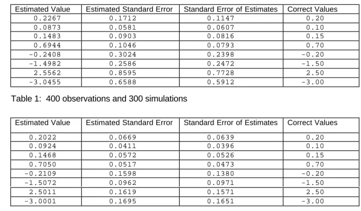
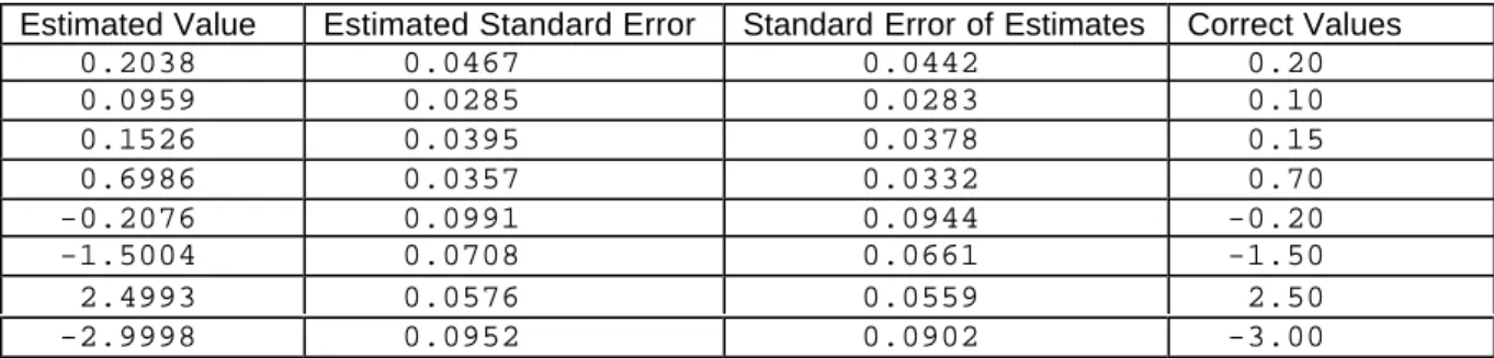
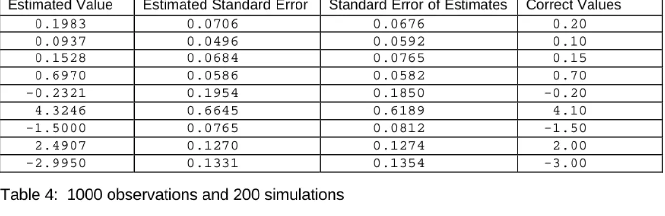
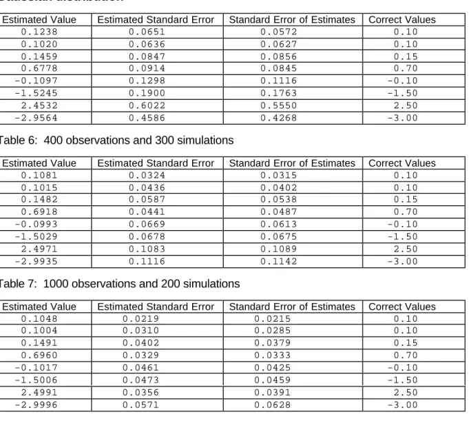
The simulation results are presented in tables 1-20 of Section 6. The first column labelled

"Estimated Value" refers to the average parameter estimate using either 300 or 200 simulations.

The second column labelled "Estimated Standard Error" refers to the average of the standard

errors computed by the GARCH software. The third column labelled "Standard Error of

Estimates" refers to the actual standard error of the parameter estimates.

(23)

6 Monte Carlo results

AGARCH-type1

The AGARCH(1,2)-type1 simulations used here had the following parameters:

The series shocks were taken from either a Gaussian distribution or a Student's

t-

distribution, with

the number of degrees of freedom

( )

df

set to 4.10.

The GARCH model parameters are output in the descending order,

α

0

,

α

1

,

α

2

,

β

1

,

γ

,

then

df

(if

present) followed by

b

i

,

i

=

1

,

K

,

3

Estimated Value

Estimated Standard Error

Standard Error of Estimates

Correct Values

0.2267

0.1712

0.1147

0.20

0.0873

0.0581

0.0607

0.10

0.1483

0.0903

0.0816

0.15

0.6944

0.1046

0.0793

0.70

-0.2408

0.3024

0.2398

-0.20

-1.4982

0.2586

0.2472

-1.50

2.5562

0.8595

0.7728

2.50

-3.0455

0.6588

0.5912

-3.00

Table 1: 400 observations and 300 simulations

Estimated Value

Correct Values

0.2022

0.0669

0.0639

0.20

0.0924

0.0411

0.0396

0.10

0.1468

0.0572

0.0526

0.15

0.7050

0.0517

0.0473

0.70

-0.2109

0.1598

0.1380

-0.20

-1.5072

0.0962

0.0971

-1.50

2.5011

0.1619

0.1571

2.50

-3.0001

0.1695

0.1651

-3.00

1

1000

2

1

100

sin

7

.

0

100

1

0

.

3

,

5

.

2

,

5

.

1

,

0

2

.

0

7

.

0

,

15

.

0

,

1

.

0

,

2

.

0

3

3 2 1 3 2 1 0 1 2 1 0

=

+

=













+

=

−

=

−

=

−

=

t t t

x

t

x

t

x

b

k

γ

α

β

α

(24)

Estimated Value

Correct Values

0.2038

0.0467

0.0442

0.20

0.0959

0.0285

0.0283

0.10

0.1526

0.0395

0.0378

0.15

0.6986

0.0357

0.0332

0.70

-0.2076

0.0991

0.0944

-0.20

-1.5004

0.0708

0.0661

-1.50

2.4993

0.0576

0.0559

2.50

-2.9998

0.0952

0.0902

-3.00

(25)

Student's

t-

distribution

Estimated Value

Correct Values

0.1983

0.0706

0.0676

0.20

0.0937

0.0496

0.0592

0.10

0.1528

0.0684

0.0765

0.15

0.6970

0.0586

0.0582

0.70

-0.2321

0.1954

0.1850

-0.20

4.3246

0.6645

0.6189

4.10

-1.5000

0.0765

0.0812

-1.50

2.4907

0.1270

0.1274

2.00

-2.9950

0.1331

0.1354

-3.00

Estimated Value

Correct Values

0.2011

0.0463

0.0456

0.20

0.0975

0.0369

0.0337

0.10

0.1523

0.0485

0.0472

0.15

0.6954

0.0379

0.0394

0.70

-0.2203

0.1338

0.1213

-0.20

4.2278

0.4241

0.4069

4.10

-1.5064

0.0524

0.0517

-1.50

2.4974

0.0451

0.0439

2.00

-2.9987

0.0743

0.0709

-3.00

(26)

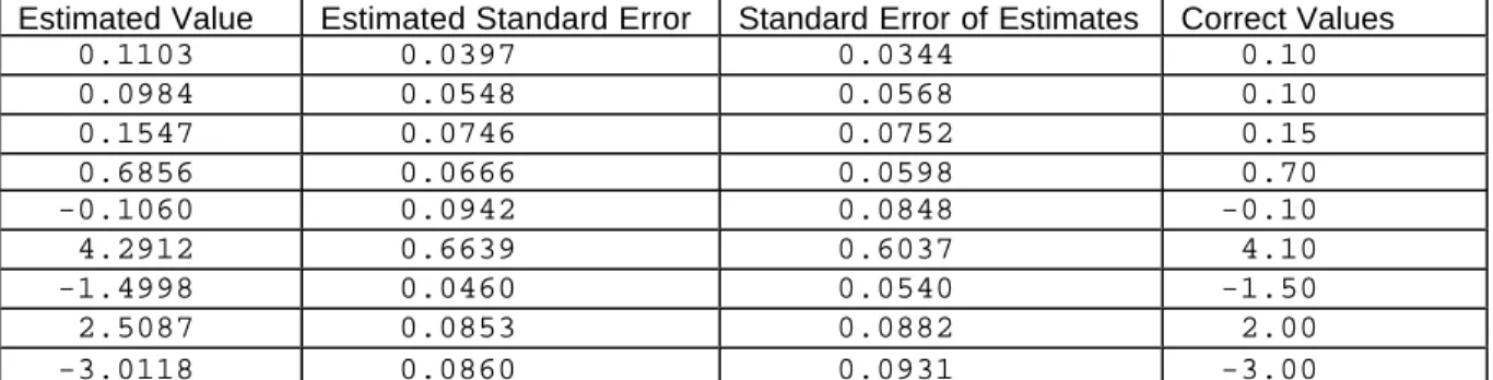
AGARCH-type2

The AGARCH(1,2)-type2 simulations used here had the following parameters:

t

-distribution, with

( )

df

set to 4.10.

The GARCH model parameters are output in the descending order,

α

0

,

α

1

,

α

2

,

β

1

,

γ

,

then

df

(if

present) followed by

b

i

,

i

=

1

,

K

,

3

Estimated Value

Correct Values

0.1238

0.0651

0.0572

0.10

0.1020

0.0636

0.0627

0.10

0.1459

0.0847

0.0856

0.15

0.6778

0.0914

0.0845

0.70

-0.1097

0.1298

0.1116

-0.10

-1.5245

0.1900

0.1763

-1.50

2.4532

0.6022

0.5550

2.50

-2.9564

0.4586

0.4268

-3.00

Estimated Value

Correct Values

0.1081

0.0324

0.0315

0.10

0.1015

0.0436

0.0402

0.10

0.1482

0.0587

0.0538

0.15

0.6918

0.0441

0.0487

0.70

-0.0993

0.0669

0.0613

-0.10

-1.5029

0.0678

0.0675

-1.50

2.4971

0.1083

0.1089

2.50

-2.9935

0.1116

0.1142

-3.00

Estimated Value

Estimated Standard Error

Correct Values

0.1048

0.0219

0.0215

0.10

0.1004

0.0310

0.0285

0.10

0.1491

0.0402

0.0379

0.15

0.6960

0.0329

0.0333

0.70

-0.1017

0.0461

0.0425

-0.10

-1.5006

0.0473

0.0459

-1.50

2.4991

0.0356

0.0391

2.50

-2.9996

0.0571

0.0628

-3.00

1

1000

2

1

100

sin

7

.

0

100

1

0

.

3

,

5

.

2

,

5

.

1

,

0

1

.

0

7

.

0

,

15

.

0

,

1

.

0

,

1

.

0

3

3 2 1 3 2 1 0 1 2 1 0

=

+

=













+

=

−

=

−

=

−

=

t t t

x

t

x

t

x

b

k

γ

α

β

α

(27)

Student's

t

-distribution

Estimated Value

Correct Values

0.1103

0.0397

0.0344

0.10

0.0984

0.0548

0.0568

0.10

0.1547

0.0746

0.0752

0.15

0.6856

0.0666

0.0598

0.70

-0.1060

0.0942

0.0848

-0.10

4.2912

0.6639

0.6037

4.10

-1.4998

0.0460

0.0540

-1.50

2.5087

0.0853

0.0882

2.00

-3.0118

0.0860

0.0931

-3.00

Estimated Value

Standard Error of Estimates

Correct Values

0.1035

0.0236

0.0221

0.10

0.1005

0.0360

0.0347

0.10

0.1528

0.0488

0.0484

0.15

0.6924

0.0417

0.0404

0.70

-0.0998

0.0599

0.0569

-0.10

4.1854

0.4345

0.3988

4.10

-1.4971

0.0324

0.0360

-1.50

2.4986

0.0284

0.0306

2.00

-2.9977

0.0441

0.0494

-3.00

(28)

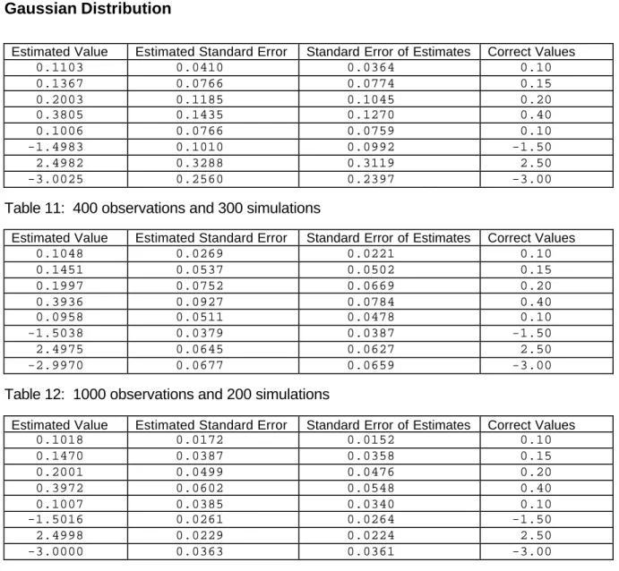
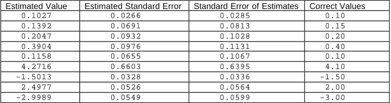
GJR-GARCH

The GJR-GARCH(1,2) simulations used here had the following parameters:

t

-distribution, with

( )

df

set to 4.10.

α

₀

,

α

₁

,

α

₂

,

β

₁

,

γ

,

then

df

(if

present) followed by

b

_i

,

i

=

1

,

K

,

3

Gaussian Distribution

Estimated Value

Correct Values

0.1103

0.0410

0.0364

0.10

0.1367

0.0766

0.0774

0.15

0.2003

0.1185

0.1045

0.20

0.3805

0.1435

0.1270

0.40

0.1006

0.0766

0.0759

0.10

-1.4983

0.1010

0.0992

-1.50

2.4982

0.3288

0.3119

2.50

-3.0025

0.2560

0.2397

-3.00

Estimated Value

Correct Values

0.1048

0.0269

0.0221

0.10

0.1451

0.0537

0.0502

0.15

0.1997

0.0752

0.0669

0.20

0.3936

0.0927

0.0784

0.40

0.0958

0.0511

0.0478

0.10

-1.5038

0.0379

0.0387

-1.50

2.4975

0.0645

0.0627

2.50

-2.9970

0.0677

0.0659

-3.00

Estimated Value

Estimated Standard Error

Correct Values

0.1018

0.0172

0.0152

0.10

0.1470

0.0387

0.0358

0.15

0.2001

0.0499

0.0476

0.20

0.3972

0.0602

0.0548

0.40

0.1007

0.0385

0.0340

0.10

-1.5016

0.0261

0.0264

-1.50

2.4998

0.0229

0.0224

2.50

-3.0000

0.0363

0.0361

-3.00

1

2

1000

1

100

sin

7

.

0

100

1

0

.

3

,

5

.

2

,

5

.

1

,

0

1

.

0

4

.

0

,

2

.

0

,

15

.

0

,

1

.

0

3

3 2 1 3 2 1 0 1 2 1 0

=

+

=













+

=

−

=

−

=

t t t

x

t

x

t

x

b

k

γ

α

β

α

(29)

Student's

t

-distribution

Estimated Value

Correct Values

0.1027

0.0266

0.0285

0.10

0.1392

0.0691

0.0813

0.15

0.2047

0.0932

0.1028

0.20

0.3904

0.0976

0.1131

0.40

0.1158

0.0655

0.1067

0.10

4.2716

0.6603

0.6395

4.10

-1.5013

0.0328

0.0336

-1.50

2.4977

0.0526

0.0564

2.00

-2.9989

0.0549

0.0599

-3.00

Estimated Value

Standard Error of Estimates

Correct Values

0.1008

0.0178

0.0170

0.10

0.1469

0.0501

0.0531

0.15

0.2016

0.0716

0.0685

0.20

0.3940

0.0683

0.0663

0.60

0.1067

0.0489

0.0606

0.10

4.2076

0.4360

0.4040

4.10

-1.4982

0.0221

0.0231

-1.50

2.4994

0.0187

0.0188

2.00

-3.0003

0.0299

0.0314

-3.00

(30)

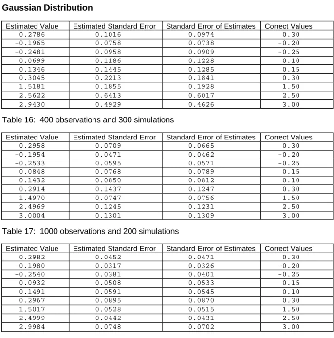
EGARCH

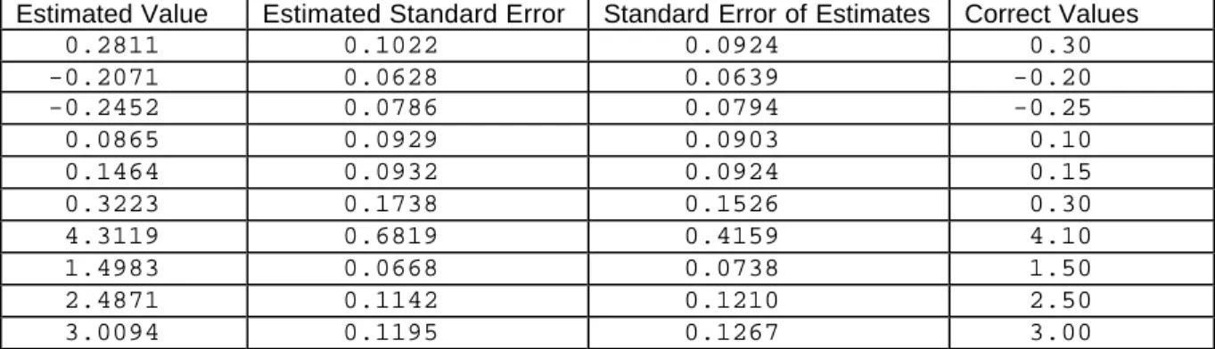
The EGARCH(1,2) simulations used here had the following parameters:

t

-distribution, with

( )

df

set to 4.10.

α

0

,

α

1

,

α

2

,

φ

1

,

φ

2

,

β

1

,

then

df

(if present) followed by

b

i

,

i

=

1

,

K

,

3

Gaussian Distribution

Estimated Value

Correct Values

0.2786

0.1016

0.0974

0.30

-0.1965

0.0758

0.0738

-0.20

-0.2481

0.0958

0.0909

-0.25

0.0699

0.1186

0.1228

0.10

0.1346

0.1445

0.1285

0.15

0.3045

0.2213

0.1841

0.30

1.5181

0.1855

0.1928

1.50

2.5622

0.6413

0.6017

2.50

2.9430

0.4929

0.4626

3.00

Estimated Value

Correct Values

0.2958

0.0709

0.0665

0.30

-0.1954

0.0471

0.0462

-0.20

-0.2533

0.0595

0.0571

-0.25

0.0848

0.0768

0.0789

0.15

0.1432

0.0850

0.0812

0.10

0.2914

0.1437

0.1247

0.30

1.4970

0.0747

0.0756

1.50

2.4969

0.1245

0.1231

2.50

3.0004

0.1301

0.1309

3.00

Estimated Value

Estimated Standard Error

Correct Values

0.2982

0.0452

0.0471

0.30

-0.1980

0.0317

0.0326

-0.20

-0.2540

0.0381

0.0401

-0.25

0.0932

0.0508

0.0533

0.15

0.1491

0.0591

0.0545

0.10

0.2967

0.0895

0.0870

0.30

1.5017

0.0528

0.0515

1.50

2.4999

0.0442

0.0431

2.50

2.9984

0.0748

0.0702

3.00

1

2

1000

1

100

sin

7

.

0

100

1

0

.

3

,

5

.

2

,

5

.

1

,

0

,

3

.

0

,

15

.

0

,

1

.

0

,

25

.

0

,

2

.

0

,

3

.

0

,

3

3 1 2 3 2 1 0 1 2 1 2 1 0

=

+

=













+

=

−

=

−

=

t t t

x

t

x

t

x

b

k

β

φ

α

(31)

Student's

t

-distribution

Estimated Value

Correct Values

0.2811

0.1022

0.0924

0.30

-0.2071

0.0628

0.0639

-0.20

-0.2452

0.0786

0.0794

-0.25

0.0865

0.0929

0.0903

0.10

0.1464

0.0932

0.0924

0.15

0.3223

0.1738

0.1526

0.30

4.3119

0.6819

0.4159

4.10

1.4983

0.0668

0.0738

1.50

2.4871

0.1142

0.1210

2.50

3.0094

0.1195

0.1267

3.00

Estimated Value

Standard Error of Estimates

Correct Values

0.2859

0.0702

0.0811

0.30

-0.2016

0.0426

0.0493

-0.20

-0.2483

0.0594

0.0706

-0.25

0.0926

0.0652

0.0657

0.10

0.1512

0.0633

0.0801

0.15

0.3154

0.1174

0.1283

0.30

4.2281

0.4348

0.3854

4.10

1.4942

0.0457

0.0539

1.50

2.4976

0.0413

0.0451

2.50

3.0001

0.0681

0.0734

3.00

(32)

Conclusions

The simulation results presented in tables 1-20 indicate that the GARCH generation and estimation

Fortran 77 software performs as expected (The forecasting software has been tested elsewhere

[9]). It was found that reliable parameter estimates and associated standard errors could only be

achieved when at least 300 observations were included in the GARCH model. More

difficult

GARCH models (those with more parameters to estimate or higher volatility memory) were found

to require even more observations to obtain consistent parameter estimates.

This report has discussed the current state of GARCH software that has been developed for Mark

20 of the NAG Fortran 77 Library. Since future modifications/improvements may take place it can

only be taken as a guide to the GARCH software that will be eventually included in the NAG

numerical libraries. Possible future improvements to the software could include the following:

•

Changing the GARCH estimation routines so that some of the model parameters can be

fixed (i.e., not estimated via maximum likelihood)

•

Other non-Gaussian shocks, such as the generalised error distribution, etc.

•

Other univariate GARCH models such GARCH-M etc.

•

Multivariate GARCH models

•

Generalising the GARCH model from regression-GARCH(

p,q

) to

ARMA(

p1,q1

)-GARCH(

p2,q2

)

Other possible modifications, concerned with language/user-interface, are as follows:

•

The inclusion of some modern Fortran features, such as memory allocation, to improve the

user-interface. Since Fortran 77 does not support memory allocation the current GARCH

software requires the user to calculate how much workspace is needed. The routines also

only allow up to 20 parameters to be estimated; this should be sufficient for most

requirements. The NAG C GARCH software, which uses internal memory allocation, does

not have these restrictions and is therefore easier to use.

•

The creation of Visual Basic wrappers which perform memory allocation and have optional

parameters etc. These could, for example, take the form of a GARCH Microsoft Excel

add-in which would have the advantage of add-interactive use and also shield users from the raw

Fortran 77 code.

•

The creation of a C++ class that contains all the GARCH functions, has optional/default

function parameters and also hides workspace, etc.

To conclude, it should be mentioned that the PC and workstation implementations of the NAG

numerical libraries permit software developers to call GARCH functions more easily than the

corresponding functions from time series packages. Although time series packages may offer the

advantage of interactive interfaces it is not easy (or computationally efficient) to call them

programmatically as a component of a larger system. The current NAG delivery mechanism is thus

well suited to software developers who want to incorporate individual GARCH routines into a new

application.

(33)

7 Acknowledgements

The author would like to thank Geoff Morgan for his help and suggestions, and also Anne

Trefethen and Neil Swindells for proof reading the manuscript.

All trademarks are acknowledged.

8 References

[1] NAG Ltd,

T