Flexible Monetary Policy Rules
Xin Xu
Thesis submitted for the degree of
Doctor of Philosophy
University of East Anglia
School of Economics
March 2017
c
This copy of the thesis has been supplied on condition that anyone who consults it is understood to recognise that its copyright rests with the author and that use of any information derived there from must be in accordance with current UK Copyright Law. In addition, any quotation or extract must include full attribution.
Abstract
The thesis includes three independent essays that investigate the properties of monetary policy rules that modern Central Banks enact in response to different shocks. Chapter 2 considers the changes observed in the policy rules followed by the Bank of England after the financial crisis in 2007. Strong evidence indicates that the linear Taylor rule is not able to capture the behaviour of the Bank of England. Considering three different types of non-linear Taylor rules – in particular, the structural model, the threshold model and the opportunistic model – we obtain robust results showing that the Bank of England has changed its policy priorities after the crisis. In Chapter 3, we compare the endogenous switching rule, in which the weights change according to the macroeconomic conditions, with the “traditional” Taylor rule with fixed weights in the basic New Keynesian model. The results show that although the endogenous-switching rule outperforms the “original” Taylor rule, the economy could benefit from implementing the linear Taylor rule by increasing the weights of inflation and output gap. Chapter 4 evaluates different monetary policy rules in a small open economy. In this framework, there exists an optimal rule which may however be hard to implement in practice. Central Banks may thus consider alternative rules. In order to minimise the welfare loss with respect to the optimal rule, we consider discretionary rules, the Taylor rule and the Taylor rule with real exchange rate, finding that the ranking of welfare performance depends on intratemporal elasticity of substitution and the degree of openness.
Contents
List of Figures iv
List of Tables v
Acknowledgements vi
1 Introduction 1
2 Modelling Bank of England’s Monetary Policy Rules before and during
the Financial Crisis 4
2.1 Introduction . . . 4
2.2 Taylor Rules . . . 5
2.2.1 General Discussion of Taylor Rules . . . 5
2.2.2 The Linear Taylor Rule . . . 6
2.2.3 Non-linear Taylor Rule . . . 7
2.3 Data . . . 10
2.4 Methodology . . . 14
2.4.1 The Linear Taylor Rule . . . 14
2.4.2 Non-linear Taylor Rules . . . 14
2.5 Empirical Results . . . 19
2.5.1 Estimating a Non-linear Taylor Rule using a Structural Model . . . 19
2.5.2 Estimating a Non-linear Taylor Rule using a Threshold Model . . . 24
2.5.3 Estimating a Non-linear Taylor Rule using an Opportunistic Model . 25 2.6 Conclusion . . . 28
3 Endogenous-switching Rules: An Evaluation 30 3.1 Introduction . . . 30
3.2 Literature Review . . . 32
3.3 The Model . . . 34
3.3.1 Households . . . 35
3.3.2 Firms . . . 36
3.3.3 Macroeconomic Equilibrium: Key Equations . . . 38
3.4.1 Social Welfare Loss Function . . . 41
3.4.2 Solution Method . . . 42
3.4.3 Alternative Monetary Policy Rules . . . 42
3.5 Numerical Analysis . . . 43
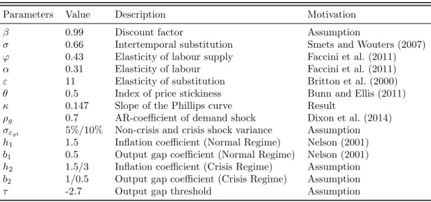
3.5.1 Calibration: Structural Parameters in the Model . . . 43
3.5.2 Calibration: Monetary Rules . . . 44
3.5.3 Results . . . 46
3.6 Conclusion . . . 56
4 Monetary Policy Rules in a Small Open Economy 58 4.1 Introduction . . . 58 4.2 Literature Review . . . 61 4.3 Model . . . 63 4.3.1 Households . . . 64 4.3.2 Firms . . . 69 4.3.3 Equilibrium . . . 71 4.3.4 Welfare . . . 75
4.4 Monetary Policy Rules . . . 76
4.4.1 Monetary Policy Rule in Foreign Country . . . 76
4.4.2 Monetary Policy Rules in Home Country . . . 76
4.5 Simulation Results . . . 81
4.5.1 Simulation Approach . . . 81
4.5.2 Calibration . . . 82
4.5.3 Rules Comparison: Discretionary Rules with Persistent Output Gaps 83 4.5.4 Rules Comparison: Discretionary Rules with One-period Output Gap 98 4.6 Conclusion . . . 107
5 Conclusion 109 Appendix A Linearisation of New Keynesian Model and Welfare around Zero Inflation Steady State 111 A.1 Linearisation of the New Keynesian Model . . . 111
A.1.1 Linearisation of the New Keynesian Phillips Curve around Zero Inflation Steady State . . . 111
A.1.2 Linearisation of IS Curve around Zero Inflation Steady State . . . . 114
A.2 Derivation the Social Welfare Loss Function . . . 115
Appendix B Linearisation of the Small Open Economy Model and Welfare117 B.1 Linearisation of the Small Open Economy Model . . . 117
B.1.1 Aggregate Demand and Real Exchange Rate . . . 117
B.1.2 Linearisation of the New Keynesian Phillips Curve around Zero Inflation Steady State . . . 118
B.1.3 Linearisation of IS Curve around Zero Inflation Steady State . . . . 121
List of Figures
2.1 The UK data . . . 13
2.2 The Bank rate and the predicted rate . . . 21
2.3 Recursive estimation of the Taylor rule . . . 23
2.4 Differences of the squared residuals between the threshold and opportunistic model . . . 28
3.1 Impulse responses to a non-crisis shock . . . 48
3.2 Impulse responses to a crisis shock . . . 51
3.3 Impulse responses to random shocks . . . 54
4.1 Foreign economy follows a negative demand shock . . . 84
4.2 Home economy in response to a foreign shock . . . 86
4.3 Welfare performance of policy rules, varying the degree of openness . . . 90
4.4 Alternative rules compared to the optimal rule, varying the degree of openness 91 4.5 Welfare performance of policy rules, varying the elasticity of substitution between home and foreign goods . . . 95
4.6 Alternative rules compared to the optimal rule, varying the elasticity of substitution between home and foreign goods . . . 95
4.7 Home economy in response to a foreign shock . . . 99
4.8 Welfare performance of simple policy rules, varying degree of openness . . . 101
4.9 Alternative rules compared to the optimal rule, varying the degree of openness101 4.10 Welfare performance of alternative policy rules, varying the elasticity of substitution between home and foreign goods . . . 103
4.11 Alternative rules compared to the optimal rule, varying the elasticity of substitution between home and foreign goods . . . 104
List of Tables
2.1 Linear Taylor rule from Q1 1992 to Q2 2013 . . . 19
2.2 Non-linear Taylor rule – the structural model . . . 20
2.3 Non-linear Taylor rule – the threshold model . . . 25
2.4 Non-linear Taylor rule – the opportunistic model . . . 26
2.5 Non-linear Taylor rule – the full opportunistic model . . . 27
3.1 Parameter values . . . 46
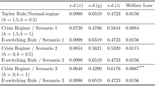
3.2 Evaluation of different policy rules under a non-crisis shock . . . 49
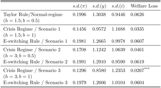
3.3 Evaluation of different policy rules under a crisis shock . . . 52
3.4 Evaluation of different policy rules under a random shock . . . 55
4.1 Simple policy rules . . . 81
4.2 Parameter values . . . 83
4.3 Standard deviations of the Home variables . . . 87
4.4 Standard deviations of the Home variables, varying the degree of openness . 92 4.5 Standard deviations of the Home variables, varying the elasticity of substitution of home and foreign goods . . . 96
4.6 Preferred policy rule, varying the degree of openness and the intratemporal elasticity of substitution . . . 98
4.7 Standard deviations of the Home variables . . . 100
4.8 Standard deviations of the Home variables, varying the degree of openness . 102 4.9 Standard deviations of the Home variables, varying the elasticity of substitution of home and foreign goods . . . 105
4.10 Preferred policy rule, varying the degree of openness and the intratemporal elasticity of substitution . . . 107
Acknowledgements
Throughout the research process, I had extremely rewarding and enjoyable years at University of East Anglia. I am deeply indebted to my supervisors Simone Valente, James Watson and Odile Poulsen, for their help, support and patience during my PhD study. Their invaluable supervision and advice provided a clear guidance for my daily research and helped this thesis improve enormously. I also grateful for the discussion and good advice during my viva by Peter Moffatt and Aditya Goenka.
I would also like to thank other faculty members, for their useful comments and suggestions. And thanks to my fellow mates and friends in the PGR office, for sharing lives with me over the past years.
I am indebted to my parents forever. Thank you for believing in me and providing unconditional support over so many years.
Chapter 1
Introduction
This thesis contains three essays on monetary policy which are motivated by the global financial crisis. It investigates the responses of monetary authority in the UK before and after the financial crisis, and exploits theoretical models to evaluate the performances of different monetary policy rules in response to different shocks.
After the global financial crisis, the UK has experienced consistent high inflation, large negative output gap and extremely low nominal interest rate. Among the many interesting research questions suggested by this experience, this thesis tackles three major issues: whether and how the Bank of England has changed behaviour, what are the consequences of switching monetary policy regimes, and which types of monetary rules are more likely to minimize welfare losses. In Chapter 2, we investigate empirically the possibility of changing behaviour in the Bank of England due to the financial crisis in 2007. The time paths of inflation, output and the Bank rate in the UK suggest the Bank of England has been more concerned about output in the post-crisis period, although it was strictly targeting inflation before 2007. Building on this observation, we consider the most recent formalizations of time-varying monetary policy rules that allow for regime change in response to changing macroeconomic conditions. We estimate non-linear Taylor rules using structural, threshold and opportunistic approaches to model the behaviour of the Bank of England. Strong
empirical evidence suggests that the preferences of the Bank of England are time-varying. The parameters in the monetary policy rule appear to have changed over time, which suggests that exogenous Taylor rule parameters are not appropriate for modelling the Bank of England over the whole time horizon considered.
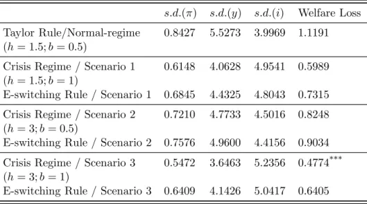
Chapter 3 studies policy change in a New Keynesian model by replacing the hypothesis of fixed policy rule with an endogenous-switching rule that allows monetary policy to change over time depending on observed shocks. Specifically, the Central Bank considers different Taylor rules and switches between them when the output gap breaches some threshold level. In addition, we evaluate the welfare performances of the “traditional” Taylor rules with different fixed weights. The endogenous-switching rule is shown to improve welfare in the event of a large negative demand shock comparing with the “original” Taylor rule. However, the “Crisis Regime” always outperforms other alternatives by showing the highest welfare although it is associated with high interest rate volatility. It suggests that a high social welfare could be achieved if Central Banks become more aggressive and raise both the weights attached to inflation and output stabilization.
An important difference between Chapters 2 and 3 is that Chapter 2 covers “positive” notions of the performance of monetary policy rules, while Chapter 3 covers “normative” notions. To be specific, in Chapter 2, a good performance of a monetary policy rule is taken to mean a close fit to the actual data, implying that the policy rule is an accurate representation of actual observed behaviour of policy-makers. In Chapter 3, in contrast, a good performance of a monetary policy rule is taken to mean that it results in a minimal welfare loss, and is hence the rule that we would advise policy-makers to use.
Chapter 4 employs a two-country dynamic general equilibrium model to examine the welfare effects of different policy responses to a Foreign demand shock in a small open economy. We evaluate monetary policy rules by using a utility-based loss function that depends on domestic inflation, output gap and real exchange rate. Using the model of
De Paoli (2009), we derive the optimal rule for a small open economy and re-express it as an interest-rate rule using the economy’s equilibrium system. When the optimal rule cannot be implemented, alternative policy rules yield different welfare levels and their ranking depends on the values taken by some key parameters – in particular, the elasticity of substitution between home and foreign goods and the degree of openness. When domestic and foreign goods are close substitutes, a discretionary rule outperforms other simple rules, while the domestic Taylor rule shows the highest welfare when the intratemporal elasticity is low. For an intermediate degree of the elasticity of substitution, the performances of alternative policy rules depends on the degree of openness.
Chapter 2
Modelling Bank of England’s
Monetary Policy Rules before and
during the Financial Crisis
2.1
Introduction
Before the financial crisis in 2007, inflation was successfully and strictly controlled by the Bank of England and there was no open letter to the Chancellor of the Exchequer. However, the post-financial crisis period is typified by slow growth, high unemployment, until recently, and relatively high inflation. High inflation led the Governor of the Bank of England to, for the first time, write open letters to the Chancellor, explaining why inflation was more than one percentage point above the inflation target. At the same time, interest rates were at record lows. The Bank of England could easily have raised rates to combat inflation but it did not, which might indicate the monetary authority have changed priorities when facing the severe shock. The research question we are interested in this Chapter is what type of the monetary policy rule could be considered as a proper way to model Bank of England behaviour when facing a severe shock. This chapter investigates various Taylor rules, modelling the Bank of England’s behaviour since 1992.
In this Chapter, we model the behaviour of the Bank of England and find changes because of the financial crisis in 2007. Using the linear Taylor rule, we find evidence that the coefficients changed significantly after the crisis, which is also proved by the recursive estimation of the Taylor rule. The empirical results present evidence that the linear Taylor rule is not able to capture the behaviour of the Bank of England, therefore, the non-linear Taylor rule is considered instead. We employ three different ways to model the non-linear Taylor rule – that is, the structural model, the threshold model and the opportunistic model, and we find strong evidence which indicates that the Bank of England behaved differently following the financial crisis shock. This Chapter provides motivation and evidence for further work that will attempt to endogenise the Taylor rule weights which policymakers put on inflation and output gaps, rather than assuming that these are independent of the size of shocks to the economy.
2.2
Taylor Rules
2.2.1 General Discussion of Taylor Rules
In his seminal paper, John Taylor (1993) proposed a formal representation of monetary policy in terms of the following rule: the Central Bank influences the nominal interest rate so as to set its value equal to a pre-determined linear function of current inflation and output gaps. In this original formulation, the Taylor rule was a positive statement, an algebraic representation of how real-world interventions were being carried over by the monetary authorities. The Taylor rule gained wide popularity as the empirical evidence confirmed its general applicability to a different economies. One of the strands of literature generated by Taylor (1993) tackled the issue of the robustness of the original rule – which specified inflation gaps in terms of deviations between current and desired inflation – by considering alternative specifications including past (so-called backward rules) and expected (so-called forward rules) inflation gaps. In this respect, several contributions suggest that backward/forward rules may fit the data better (Svensson, 2003; Benhabib et al., 2001; Clarida et al., 1998; Carlstrom et al., 2000). However, the robustness of
Taylor’s original rule may be assessed with respect to other characteristics: in the present Chapter, we do not consider the extensions to backward/forward rules and focus, instead, on possible non-linearities. More precisely, we investigate the possibility that a simple non-linear rule fits the data better than the traditional linear specification.
2.2.2 The Linear Taylor Rule
Taylor (1993) examined the performance of monetary policy across the G-7 countries, and found that the movements of the Federal fund rates from 1987 to 1992 were quite consistent with the estimates of the rule. Although the estimated period is just a short period, the good performance of the rule has made it to be one of the standard ways to describe monetary policy. Therefore, he suggests that a rule that moves the nominal interest rate in response to the deviation of inflation and output gap could provide a standard guidance for Central Banks to set monetary policy, which is the well-known “Taylor Rule”. In the original Taylor (1993) paper, the policy rule reads
it =πt+rnaturalt +h(πt−πtT) +b(yt−yTt) (2.1)
where it is the short-term nominal interest rate, rtnatural is the natural interest rate,
πt is inflation, yt is the logarithm of real GDP, and the πtT and yTt are policy targets.
The coefficients h and b are the weights that Central Banks put on stabilising inflation and minimising the output gap respectively – a relatively higher h suggests a more inflation-averse Central Bank; while a higher b suggests a Central Bank more willing to loosen/tighten monetary policy when output is below/above potential.
Taylor (1993) points out that Central Banks could follow an exact rule when setting the monetary policy, which suggests that the natural interest rate and inflation target take constant values (rnatural = 2, πT
t = 2), and the coefficients on the deviation of inflation
from target and of output from its natural rate are constant over time and equal to 0.5. Taylor (1999b) tests the efficiency and robustness of the “original” linear rule and finds
evidence that it could be used as a guideline for the European Central Bank. The good performance of the linear Taylor rule has been demonstrated by substantial studies, particularly, it shows that the Taylor rule works nearly as well as an optimal monetary policy rule (see e.g. Rudebusch and Svensson, 1999; Woodford, 2001; Ball, 2012). Also, Levin et al. (1999) state that the linear rule works better and perform more robustly than a complicated rule. It seems that the economic movements will be less unlikely to have a bad performance as long as the parameters in the Taylor rule are assigned appropriate weight. One advantage of the Taylor rule is that the rule is straightforward, it only requires current inflation and the inflation target and the output gap.
Although the Taylor rule could describe a monetary policy properly in normal times and over definite time periods, Taylor (1993) himself made it clear that the rule is too simple to capture the behaviour of Central Banks facing changing economic conditions that would likely induce monetary authorities to change the conduct of monetary policy. ¨Osterholm (2005) shows the Taylor rule is not able to fit the data completely, indicating Central Banks behave in a more sophisticated way than just following a simple instrument rule. Furthermore, Orphanides (2003) states that although a Taylor rule could be a useful tool for interpreting historical policy, strong evidence shows that it is not possible to have a stable monetary policy over time as policymakers would not have sufficient knowledge to assess the movement of the economy in the future. And Svensson (2003) argues that when setting the nominal interest rate, more variables should be taken into consideration than just inflation and the output gap.
2.2.3 Non-linear Taylor Rule
Asymmetric preferences in the behaviour of Central Banks have been argued by literature. Dolado et al. (2004) show that the Fed behaved more aggressively when there are positive inflation deviations from its target than negative ones, during the Volcker-Greenspan period. Lo and Piger (2005) find that output reacts more to policy actions during recessions than expansions, which is also supported by Peersman and Smets (2001), who
show evidence that there are significantly stronger effects on output in recessions than in booms in the Euro area, indicating Central Banks implement asymmetric preferences towards prices and aggregate demand under different economic conditions. Similar results have been found in the UK and US by Cukierman and Muscatelli (2008) and in the US by Rudebusch and Svensson (1999). Therefore, non-linear interest rate reaction functions are considered in studies as it is required when modelling the asymmetry in Central Banks’ behaviour (Taylor and Davradakis, 2006).
In the original paper of Taylor (1993), a short period in the US, from 1987 to 1992, was estimated and showed good performance of the Taylor rule. Not surprisingly, it is not sensible to assume the policymakers would follow a simple rule over time. Clarida et al. (2000) separate US data into three sample periods, Pre-Volcker, Volcker-Greenspan and Post-82, and then apply a forward-looking Taylor rule. And the results show that the estimated coefficients are sensitive to the sample estimation period employed. This is also confirmed by the results shown by Hamalainen et al. (2004) and Judd and Rudebusch (1998), where estimate Taylor rules for different periods and find the Fed reacted differently towards inflation and output over time.
Clearly, the linear Taylor rule is not able to capture the movement of nominal interest rates over long time periods. As much literature shows that the estimated weights on inflation and output may be sensitive to policy regime, it may suggest the possibility of structural breaks (Siklos and Wohar, 2005). This has been proved by Nelson (2001), who find evidence of structural breaks when estimating the UK monetary policy from 1972 to 1997, by separating the sample period into several regimes.
Cukierman and Muscatelli (2008) estimate a non-linear Taylor rule using a smooth-transition model. As the observed Bank rate in the UK drops from 5.25% to 0.5% within a year (from March 2008 to March 2009), the smooth-transition model is not a proper way to model the non-linear Taylor rule as it requires smooth changes in the nominal interest rate. Instead, a
threshold model allows abrupt changes from one regime to another. Taylor and Davradakis (2006) point out that a simple way to describe nonlinearities is to estimate a threshold model, which has been applied to the UK from 1992 to 2003. Bunzel and Enders (2010) have argued that the loss function of Central Banks is likely to be asymmetric around inflation and output gaps. The Fed would be more aggressive when inflation is 1% above the target than 1% below target. Similarly, negative values of output gap are viewed as more problematic than the positive values of output gap. So these types of nonlinearities would imply that some threshold model is reasonable.
Cukierman and Muscatelli (2008) argue that the loss function of Central Banks could be asymmetric which refer to recession-avoidance preferences and inflation-avoidance preferences. Blinder (1999) states that in most situations Central Banks will take more political action when trying to avoid higher inflation than avoiding higher unemployment, suggesting that the negative output gap draws more attention than when there is a positive output gap. Taylor and Davradakis (2006) have modelled the Bank of England’s behaviour using a non-linear Taylor rule and used threshold models to capture nonlinearities in policy behaviour. The policy rule switches when a certain value breaches the threshold. In their model, the interest rate is implemented under different Taylor rules when inflation is below or above threshold. The results show that a Taylor rule with a specified threshold is a proper way to describe the movement of the nominal interest rate.
Bunzel and Enders (2010) apply a non-linear Taylor rule using a threshold model to the US data and find strong evidence of threshold behaviour in most of the periods, either using the inflation rate or the output gap as a threshold. Then, the threshold model has been applied to several sub-periods of the US data using lagged inflation rate as threshold. The results suggest that the Fed responds much more strongly to the movement of inflation and output when inflation exceeds the threshold value.
Instead of using a deliberate inflation target, by implementing an “opportunistic strategy”, opportunistic policymakers use an interim inflation target which may simply be the current
inflation rate and use the effect of shocks to reduce inflation and eventually achieve the ultimate inflation target. The opportunistic rule allows monetary authorities to alter their priorities depending on movements of inflation and output gap. The advantage of opportunistic disinflation has been argued by Aksoy et al. (2006), who find that although it takes longer time to achieve disinflation using an opportunistic strategy, it requires smaller output losses than using a deliberate approach. Bomfim and Rudebusch (2000) estimates opportunistic monetary policy using the Taylor rule with an interim inflation target. The results show that as long as inflation is stable, where the current inflation is similar with a previous rate, the opportunistic policymaker will not take any action to reduce it.
The main insight of these empirical literature is that Central Banks react to changing economic conditions by “adjusting the weights” attached to output and inflation stabilization – that is, Central Banks update their priorities when the economy hit by severe shocks. However, the majority of these studies investigate the period before the financial crisis in 2007. In contrast, the present analysis includes both the period before and after 2007, and studies whether and how the policy rule has changed after the severe demand shock induced by the crisis.
2.3
Data
On 8thOctober 1992, the UK monetary policy adopted a framework of inflation targeting
and the first inflation target was announced. From that time the Bank of England started to target inflation at 2.5%, which is measured by RPIX (the Retail Price Index (RPI) excluding mortgage interest payments). The final decision on interest rates was not set by the Bank of England until May 1997, when the new Monetary Policy Committee (MPC) was given the power to set the official interest rate monthly. In December 2004, the inflation target changed from 2.5% RPIX to 2% CPI (Consumer Price Index).
Before the financial crisis, much of the interim period the Bank of England moved the nominal interest rates slightly, and was able to keep inflation close to the target. While, in response to the recent financial crisis the Bank of England reduced the policy interest rate to 0.5%, complemented by£375bn of further monetary easing, popularly known as Quantitative Easing, which attempts to further stimulate the economy when conventional monetary policy becomes ineffective. The reduction of interest rates to such levels is unprecedented, having never previously been below 2% since the Bank of England was founded in 1694.
Meanwhile, the rate of inflation in the UK has spent much of recent years above target. If inflation is within 1% change in either direction, the deviation from the inflation target could be tolerated. Inflation more than 1% above the target has led to a series of open letters, from April 2007 to February 2012.
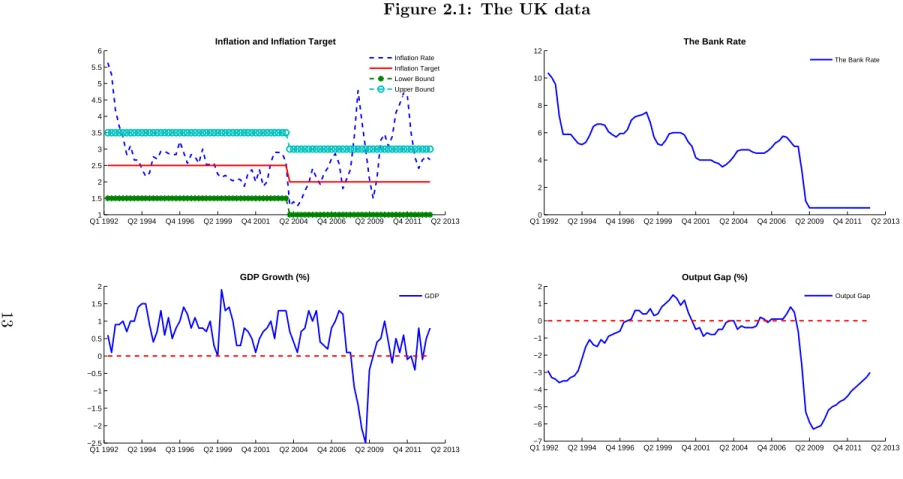
The data used to estimate the Taylor rule is quarterly data from the first quarter in 1992 until the second quarter in 2013. Figure 2.1 shows the quarterly data of the UK inflation, GDP, the output gap and the Bank Rate from 1992 to the second quarter in 2013. The monthly Bank rate for the whole period is available from the Bank of England. The inflation on a monthly basis (RPIX and CPI), which is measured by percentage change on the same period of the previous year, is available from the Bank of England. The output gap is constructed by the deviation of real output from potential output. The output gap used is published quarterly by the Office for Budget Responsibility.
The inflation gap is measured as the deviation of inflation from target. The first inflation target was 2.5% annually measured by RPIX which started in 1992. This situation continued for 12 years, until the new inflation target was announced in December 2003. Since then, the inflation measurement changed to CPI and the target changed to 2% annually. Throughout the entire period, the inflation rate is measured by the appropriate method (RPIX and CPI respectively), and along with the corresponding inflation target
Figure 2.1: The UK data Q1 19921 Q2 1994 Q4 1996 Q2 1999 Q4 2001 Q2 2004 Q4 2006 Q2 2009 Q4 2011 Q2 2013 1.5 2 2.5 3 3.5 4 4.5 5 5.5 6
Inflation and Inflation Target
Inflation Rate Inflation Target Lower Bound Upper Bound Q1 19920 Q2 1994 Q4 1996 Q2 1999 Q4 2001 Q2 2004 Q4 2006 Q2 2009 Q4 2011 Q2 2013 2 4 6 8 10 12
The Bank Rate
The Bank Rate
Q1 1992 Q2 1994 Q3 1996 Q2 1999 Q4 2001 Q2 2004 Q4 2006 Q2 2009 Q4 2011 Q2 2013 −2.5 −2 −1.5 −1 −0.5 0 0.5 1 1.5 2 GDP Growth (%) GDP Q1 1992−7 Q2 1994 Q4 1996 Q2 1999 Q4 2001 Q2 2004 Q4 2006 Q2 2009 Q4 2011 Q2 2013 −6 −5 −4 −3 −2 −1 0 1 2 Output Gap (%) Output Gap 13
2.4
Methodology
2.4.1 The Linear Taylor Rule
The Taylor rule is a popular way of modelling Central Banks’ behaviour. The rule assumes that the nominal interest rates are set in respect to some weighted combination of inflation and output from the trend. The linear Taylor Rule reads:
it=α+h(πt−πtT) +b(yt−yTt) (2.2)
The Taylor rule describes the change of nominal interest rate based on the deviation between the actual inflation rate and inflation target, and the divergence of actual GDP from potential GDP. The implication of the Taylor rule is that the parameters on these two gaps are decided directly by the policymakers. Central Banks can put their preferences into practice by choosing these parameters in order to attempt to improve economic performance.
2.4.2 Non-linear Taylor Rules
Expression (2.2) assumes constant weights attached to inflation and output gaps over time, which excludes the possibility of regime changes when Central Banks face unexpected events such as demand shocks of large magnitude. However, the behaviour of the Bank of England since the global financial crisis is strongly suggestive of the weights changing in response to a severe shock.
From the analytical point of view, abrupt changes in the policy rule may be formalized as “non-linearities” in the Taylor rule. In this Chapter, we consider non-linearities in Taylor-type rules allow a switch is different linear Taylor rules as determined by some condition such as a threshold or a structural break, which is commonly used in the literature. It is important to not confuse this terminology with a Taylor rule that is non-linear in the curved sense – e.g. being a polynomial of some degree higher than unity.
The Structural Model
The time paths of nominal interest rate, inflation and output gap are shown in Figure 2.1. In order to capture the features of the economy before and after the crisis, the possibility of structural break could be taken into consideration. Therefore, we estimated the Taylor rules for the entire period as well as two sub-periods based on the beginning of the economic crisis in the second quarter of 2007. The reason behind this is that March 2007 was the first time that inflation went over 1% above the target since the inflation target was introduced.
The structural model takes the form
it= α1+h1(πt−πtT) +b1(yt−ytT) if t <T¯ α2+h2(πt−πtT) +b2(yt−ytT) if t≥T¯ (2.3)
where ¯T is the structural break date, which we choose the second quarter of 2007. Coefficients
α1, h1 and b1 are estimates when t < T¯, while coefficients α2, h2 and b2 are estimates otherwise.
The Threshold Model
The threshold regression was original developed by Hansen (1997), which allows two linear Taylor rules to switch as determined by the threshold value, ˆτ.
Assume that the dependent variable isYt= h
y1 y2 ... yn i
, a set of independent variable isXt=
h
x1 x2 ... xn i
. The Taylor rule threshold regression model takes the form
it= [α1+h1(πt−πTt)+b1(yt−ytT)]I(qt−d≤τˆ)+[α2+h2(πt−πtT)+b2(yt−ytT)]I(qt−d>τˆ)+µt
(2.4) whereqt−d is the threshold variable in periodt−d,I(·) is the indicator function and the
Or, it could be written as it= α1+h1(πt−πtT) +b1(yt−ytT) if qt−d≤τˆ α2+h2(πt−πtT) +b2(yt−ytT) if qt−d>τˆ (2.5)
Threshold Value Estimation
The threshold model allows the regression parameters to change depending on the threshold. Therefore, the threshold value needs to be estimated first. According to Hansen (1997), the appropriate estimation method is least squares. The practical approach of finding the threshold is as follows. First, form a potential threshold value set, Γ, using the value of
qt−dwhich eliminates the highest and lowest 15% of the sortedqt−d, wheret= 1...n. Then
run Generalized Method of Moments (GMM) regressions of the form of equation (2.5), setting τ =qt−d, for each τ ∈Γ. And the sum of squared residuals obtained. The ˆτ can
be found when the lowest sum of residuals variance appears, which can be expressed as
ˆ
τ =argminτ∈Γσˆn2(τ)
In this Chapter, we assume the output gap and inflation gap as threshold variables. Set
τ =qt−1, whereqt−1 is assumed to beyt−1 andπt−1 respectively. Then follow the method of Hansen (1997). The value of ˆτ is associated with the lowest sum of residuals variance.
Test for a Threshold
It is important to know whether the threshold model of the Taylor rule (2.5) is statistically significant from a linear model. So, next we discuss about the test for a threshold.
The null hypothesis of the no threshold effect in the model is H0:A1=A2 whereA1 = h α1 h1 b1 i′ andA2= h α2 h2 b2 i′
The alternative hypothesis of threshold effect is
H1 :A16=A2
As the threshold value is an unknown parameter under the null hypothesis, a standard F-test is not suitable for this case. Instead, in order to test threshold behaviour, Hansen (1997) pointed out that it is necessary to bootstrap the F-statistic, and the procedure is as follows. In this Chapter, the bootstrap F-test is conducted in STATA.
First, the model is estimated by least squares for each τ ∈ Γ and the sum of squared residuals obtained. So, the pointwise F-statistic is formed:
Fn(τ) =n [˜σ2 n−σˆn2(τ)] ˆ σ2 n(τ) where ˜σ2
nis obtained from the linear Taylor rule, and ˆσ2n(τ) is obtained from the threshold
model.
Then the bootstrap F-statistic is the largest value of these statistics, which can be expressed as:
Fn=supτ∈ΓFn(τ)
In order to achieve the p-value for F-statistic, a bootstrap procedure has been proposed by Hansen (1997). Detailed process is letu∗t bei.i.d. N(0,1) random draws, and obtain ˆet
from the estimation of the threshold model. Then sety∗
the residual variance ˜σ∗2
n , and regressyt∗ on Xt(τ) to obtain the residual variance ˆσn∗2(τ).
Then form Fn∗ =n[˜σn2∗−σˆ ∗2 n(τ)] ˆ σ∗2 n(τ) and F ∗
n =supτ∈ΓFn∗(τ) is obtained. Finally, the bootstrap
p-value of the test is formed by counting the percentage of bootstrap samples for which
Fn∗ exceeds the observed Fn.
The Opportunistic Model
As the inflation in the UK was being consistent high after the financial crisis, it seems that the inflation target is not followed strictly by the Bank of England, which makes it interesting to investigate opportunistic monetary policy. According to Bunzel and Enders (2010), the opportunistic policy assumes the interim inflation target is changing over time, in this Chapter, we estimate the monetary rule using an interim target rate instead of using a fixed threshold. Assume that there is a regime change if the current inflation gap breaches the average rate of the last two years. The non-linear Taylor rule using opportunistic approach can be expressed as
it= α1+h1(πt−πTt) +b1(yt−ytT) if (πt−1−πtT−1)≤ (πt−5−πtT−5)+(πt−9−πTt−9) 2 α2+h2(πt−πTt) +b2(yt−ytT) if (πt−1−πtT−1)> (πt−5−πtT−5)+(πt−9−πTt−9) 2 (2.6) The opportunistic model allows policy regime changes between two linear Taylor rules based on a changing threshold. Furthermore, the full opportunistic model takes the output gap into consideration, it takes the same model shown in expression (2.6) but with a different indicator function. Specifically, the full opportunistic model reads:
it= α1+h1(πt−πtT) +b1(yt−ytT) if (πt−1−π T t−1)≤ (πt−5−πTt −5)+(πt−9−πTt −9) 2 &(yt−1−y T t−1)>0 α2+h2(πt−πtT) +b2(yt−ytT) if (πt−1−π T t−1)> (πt−5−πTt −5)+(πt−9−πTt −9) 2 &(yt−1−y T t−1)≤0 (2.7)
2.5
Empirical Results
2.5.1 Estimating a Non-linear Taylor Rule using a Structural Model
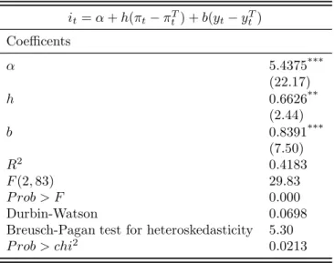
Before breaking the data into sub-periods, first we estimate the original Taylor rule for the whole sample. Table 2.1 reports the estimated linear Taylor rule since 1992 by using Ordinary Least Square (OLS).
Table 2.1: Linear Taylor rule from Q1 1992 to Q2 2013 it=α+h(πt−πtT) +b(yt−yTt) Coefficents α 5.4375*** (22.17) h 0.6626** (2.44) b 0.8391*** (7.50) R2 0.4183 F(2,83) 29.83 P rob > F 0.000 Durbin-Watson 0.0698 Breusch-Pagan test for heteroskedasticity 5.30
P rob > chi2 0.0213 Notes: T-statistics are reported in parentheses. The superscript * indicates significance (p-value<0.1); ** indicates strong significance (p-value<0.05); *** indicates very strong significance (p-value<0.01). The model is estimated by OLS.
The results show coefficients obtained in the linear rule are quite consistent with the values suggested by Taylor (1993), which is confirmed by an F-test. However, the results are not efficient as the data suffers from a high degree of autocorrelation (Durbin-Watson statistic = 0.0698). And the heteroskedasticity causes the poor performance of the regression. A Chow test for structural break suggests that the parameters are not constant over time (F-statistic = 29.83 with a p-value of 0.000). Therefore, we spilt the data into two sub-periods and choose March 2007 as the break point.
As the data has the problem of autocorrelation and heteroskedasticity, OLS becomes inefficient and results are not the “best linear unbiased estimator”. Therefore, instead of using OLS, we use Generalized Method of Moments (GMM) which can give robust results
and the corrected standard errors are known as “heteroscedasticity-and autocorrelation-consistent” (HAC) standard errors. Table 2.2 reports the estimated Taylor rule before and after the
financial crisis.
Table 2.2: Non-linear Taylor rule – the structural model it= α1+h1(πt−πTt) +b1(yt−ytT) if t <T¯ α2+h2(πt−πTt) +b2(yt−ytT) if t≥T¯ Start End α1 h1 b1 R2 Q1 1992 Q1 2007 5.4287*** 1.5419*** 0.1276 0.4810 (35.37) (8.56) (1.32) α2 h2 b2 R2 Q2 2007 Q2 2013 4.8215*** -0.1386 0.8247*** 0.8461 (16.52) (-0.87) (14.89)
Notes: Z-statistics are reported in parentheses. The superscript * indicates mild significance (p-value<0.1); ** indicates significance (p-value<0.05); *** indicates strong significance (p-value<0.01). The model is estimated by GMM.
Generally, if a linear Taylor rule appropriately describes the behaviour of the Bank of England, the estimated parameters should be constant over time. However, the estimates on inflation become insignificant while output estimates become significant when moving to the post-crisis period. This suggests that the behaviour changed significantly after the crisis, indicating that the Bank of England does not follow a linear rule all the time. Table 2.2 shows that coefficients for the first period are both positive and the inflation gap has a very strong significant number (p-value=0.000) which suggests that the Bank of England cared more about inflation before the financial crisis started. Moreover, it seems that the Bank of England followed the “Taylor Principle” as the coefficient on the inflation gap is greater than 0.5. Interestingly, this coefficient changed to a negative but not significant number, so there is no evidence to show the Bank of England continues to put
a strong weight on inflation since the crisis. Instead, a very significant positive coefficient is estimated on output gap (p-value=0.000), suggesting that the Bank of England changed preference and started to care more about output.
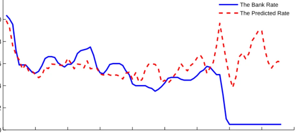
Figure 2.2 shows the path of nominal interest rates assuming the pre-2007 Taylor rule parameters presented in Table 2.2. The predicted rates are calculated using estimates obtained from the first period, shown as equation (2.8). The observable differences between these two rates give further evidence that the Bank of England behaved differently after the crisis.
ipredictt = 5.4287 + 1.5419(πt−πTt) + 0.1276(yt−yTt) (2.8)
Figure 2.2: The Bank rate and the predicted rate
Q1 19920 Q2 1994 Q4 1996 Q2 1999 Q4 2001 Q2 2004 Q4 2006 Q2 2009 Q4 2011 Q2 2013 2 4 6 8 10 12
The Bank Rate The Predicted Rate
In order to test whether the coefficients of the estimated Taylor rule are constant over time statistically, a standard recursive estimation method has been used. To be precise, for each timeT in the time period of Q2 2007 to Q2 2013, the linear Taylor rule is estimated using the observations from Q1 1992 to T. Therefore, there are 25 regressions and each has coefficients on inflation and output gap and an intercept. The results are shown in
Figure 2.3. Figure 2.3 shows the parameter movements when one single policy regime is used to describe the data from 1992 to 2013. If the parameters are constant over time, there should be no particular pattern observed in the coefficients. However, none of those coefficients are constant over time.
Specifically, there is a fall in all coefficients and intercept around 2008. After that the output gap coefficient increases gradually over time, while the coefficient of inflation gap decreased gradually since the last quarter of 2009. The results give further evidence that the policy priority of the Bank of England has changed over time – that is, a linear Taylor rule is not able to describe the behaviour of the Bank of England appropriately. Therefore, it is necessary to consider non-linear Taylor rules.
Figure 2.3: Recursive estimation of the Taylor rule Q2 20070.4 Q2 2008 Q3 2009 Q4 2010 Q1 2012 Q2 2013 0.6 0.8 1 1.2 1.4 1.6 1.8 2
Inflation Gap Coefficient
Inflation Gap Coefficient
Q2 2007 Q2 2008 Q3 2009 Q4 2010 Q1 2012 Q2 2013 −0.2 0 0.2 0.4 0.6 0.8 1 1.2
Output Gap Coefficient
Output Gap Coefficient
Q2 2007 Q2 2008 Q3 2009 Q4 2010 Q1 2012 Q2 2013 5.35 5.4 5.45 5.5 5.55 Intercept Intercept 23
2.5.2 Estimating a Non-linear Taylor Rule using a Threshold Model
In the UK, the economy has experienced negative output gaps from 2008 to 2013. As shown from the recursive estimation, the Bank of England started to put more weight on output, relaxing the control of inflation at the same time. In order to investigate more about the monetary policy rule in the UK, the threshold model (2.3) will be applied to the UK economy next.
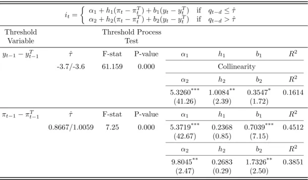
Table 2.3 reports the estimated non-linear Taylor rule using a threshold model which adopts the lagged output gap and inflation gap as threshold variables. No matter which threshold variable is chosen, there is strong evidence of threshold behaviour in the sample, indicating that a linear Taylor rule is not being employed. The two estimates of ˆτ are the estimation range of each threshold variable, indicating the Bank of England would follow a different rule when the lagged inflation gap (lagged output gap) crosses that value. The estimates show that when the lagged output gap is above the threshold value, it seems that the Bank of England followed the Taylor principle. However, when the lagged output gap is below the threshold, the model can not be estimated due to collinearity. This can be explained as most of the data in this sample falls into the post-crisis period which the structural model suggests. Specifically, most of the dependent variables are constant, having the nominal interest rate at 0.5%. There are more evidence that the regime has changed significantly when the lagged output gap is below the threshold value, but that this coincides with the post-financial crisis period.
Instead, if we assume the lagged inflation gap as the threshold variable, the coefficient on output gap has increased sharply when the lagged inflation gap is above the threshold value. Interestingly, this is opposite of what we might expect. When the inflation gap is above the threshold, the Central Bank is supposed to put more effort on controlling the rate of inflation, but it did not. The output-preferred behaviour may be triggered by recessions or shocks which could make the Bank of England focus on output in order to
get the economy back on track. Correspondingly, when the lagged inflation gap is above the threshold, most of the data refer to the period after the financial crisis, when there is strong evidence from the recursive estimation that the Bank of England is putting more weight on output. It seems that the results are plausible.
Table 2.3: Non-linear Taylor rule – the threshold model
it=
α1+h1(πt−πtT) +b1(yt−ytT) if qt−d≤τˆ
α2+h2(πt−πtT) +b2(yt−ytT) if qt−d>τˆ Threshold Threshold Process
Variable Test yt−1−y T t−1 τˆ F-stat P-value α1 h1 b1 R 2 -3.7/-3.6 61.159 0.000 Collinearity α2 h2 b2 R2 5.3260*** 1.0084** 0.3547* 0.1614 (41.26) (2.39) (1.72) πt−1−π T t−1 τˆ F-stat P-value α1 h1 b1 R 2 0.8667/1.0059 7.25 0.000 5.3719*** 0.2368 0.7039*** 0.4512 (42.67) (0.85) (7.15) α2 h2 b2 R2 9.8045** 0.2683 1.7326** 0.3851 (2.47) (0.29) (2.50)
Notes: Z-statistics are reported in parentheses. The superscript * indicates mild significance (p-value<0.1);** indicates significance (p-value<0.05);*** indicates strong significance (p-value<0.01). F-stat and P-value are calculated using bootstrap procedure described in section 2.4.2. The model is estimated by GMM.
2.5.3 Estimating a Non-linear Taylor Rule using an Opportunistic Model
Instead of assuming Central Banks use a fixed threshold, next we will consider whether Central Banks could change their behaviour based on a changing threshold, which is commonly known as “Opportunism”.
Table 2.4 shows the results if the Taylor rule for the UK is viewed as an opportunistic strategy process, which is shown as expression (2.6). When the lagged inflation gap is
lower than the threshold, the Bank of England responds significantly to inflation and output. This may indicate that the Bank of England controls inflation strictly to its target rate when the economy behaves normally. Interestingly, the results indicate the Bank of England responds less to the inflation and coefficient of inflation gap becomes insignificant when the lagged inflation gap is above the average inflation rate of the last two years. This is quite unusual as it seems that the Bank of England should care more about inflation when it becomes higher than threshold. Instead, the results show a very strong significant effort has been put on output. The results are quite consistent with the threshold model.
Table 2.4: Non-linear Taylor rule – the opportunistic model
it= ( α1+h1(πt−πtT) +b1(yt−ytT) if (πt−1−π T t−1)≤ (πt−5−πTt −5)+(πt−9−πTt −9) 2 α2+h2(πt−πtT) +b2(yt−ytT) if (πt−1−π T t−1)> (πt−5−πTt −5)+(πt−9−πTt −9) 2 Threshold Variable πt−1−π T t−1 α1 h1 b1 R 2 5.6641*** 1.7968*** 0.8562*** 0.4711 (30.60) (4.36) (6.33) α2 h2 b2 R2 5.3537*** -0.0743 0.8964*** 0.7763 (22.88) (-0.53) (16.82)
Notes: Z-statistics are reported in parentheses. The superscript * indicates mild significance (p-value<0.1); ** indicates significance (p-value<0.05); *** indicates strong significance (p-value<0.01). The model is estimated by GMM.
As there is a strong significant result estimated on output, it is reasonable to assume the output gap to be one of the thresholds. Therefore, we estimate the “full” opportunistic model (2.7), which implies policy changes rely on two thresholds: inflation gap and output gap.
After the financial crisis, the UK experienced consistently high inflation and negative output gaps, therefore, in this Chapter, we try to capture the UK experience using the
full opportunistic model. In particular, we assume there will be a policy regime change when the inflation gap is above the threshold and the output gap is below zero in the full opportunistic model. Table 2.5 shows the estimates of the UK data under the full opportunistic model. When the inflation gap is above the threshold and the output is lower than zero, the coefficient of output gap raises sharply and becomes strongly significant, which indicates that the Bank of England cares much more about output than inflation when the inflation gap is less than threshold and output gap is more than threshold.
Table 2.5: Non-linear Taylor rule – the full opportunistic model
it= ( α1+h1(πt−πtT) +b1(yt−yTt) if (πt−1−π T t−1)≤ (πt−5−πT t−5)+(πt−9−πT t−9) 2 &(yt−1−y T t−1)>0 α2+h2(πt−πtT) +b2(yt−yTt) if (πt−1−π T t−1)> (πt−5−πT t−5)+(πt−9−πT t−9) 2 &(yt−1−y T t−1)≤0 Threshold Variable πt−1−π T t−1&yt−1−y T t−1 α1 h1 b1 R 2 6.6861*** 0.1522 -0.9235 0.5923 (14.34) (0.20) (-1.40) α2 h2 b2 R2 5.3209*** -0.1272 0.8695*** 0.7664 (17.74) (-0.72) (12.62)
Notes: Z-statistics are reported in parentheses. The superscript* indicates mild significance (p-value<0.1); **
indicates significance (p-value<0.05); *** indicates strong significance (p-value<0.01). The model is estimated by GMM.
Based on the estimates obtained from the threshold and opportunistic models, significant coefficients are shown on output gap in high inflation regimes, which probably could be explained by the financial crisis. After the financial crisis in 2007, the Bank of England is not able to maintain the “normal” policy as they have to deal with the recession. Thus, the Bank of England has to put more weight on output in order to eliminate the negative output gap even if there is pressure on prices, which is consistent with the results obtained from the structural model.
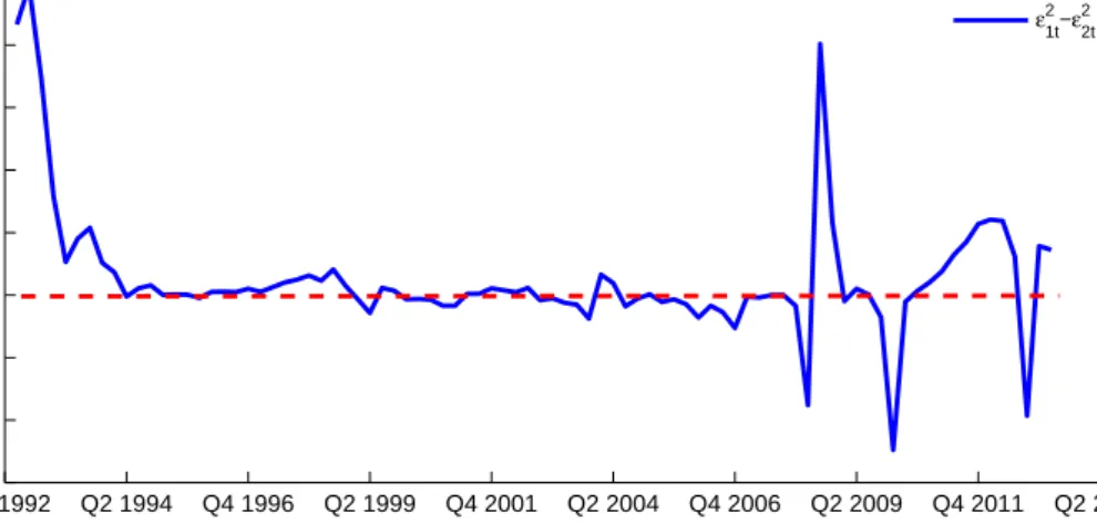
In order to see whether the Bank of England follows a threshold process or tends to behave based on an opportunistic strategy, it is necessary to compare the performance of the two models. Figure 2.4 shows the differences between the threshold model and
the opportunistic model. Let {ε2
1t} represents the sequence of squared variances from the
threshold model and let{ε22t} be the sequence of squared variance from the opportunistic model. Figure 2.4 showsε2
1t−ε22t during the period of 1992 to 2013 second quarter. Figure 2.4: Differences of the squared residuals between the threshold and opportunistic model Q1 1992 Q2 1994 Q4 1996 Q2 1999 Q4 2001 Q2 2004 Q4 2006 Q2 2009 Q4 2011 Q2 2013 −15 −10 −5 0 5 10 15 20 25 ε1t2 −ε2t2
Positive numbers occur in the period before 1994 and after 2008, indicating that the behaviour of the Bank of England is better described using an opportunistic model. After that, it is quite consistent for the two models until 2008. After 2008, it is complicated but the opportunistic model is better for most periods, which is also supported by the R-squared estimates in both models. Moreover, the opportunistic model seems more realistic as the policymakers will not take any action to inflation as long as inflation is stable even it stays beyond the band, which is quite consistent with the experience in the UK since 2008.
2.6
Conclusion
This chapter discusses ways of modelling the Bank of England’s behaviour using different Taylor-type rules. We estimate a standard linear Taylor rule for the whole period, which
shows strong evidence of a structural break. Due to the instability existing in the parameters, non-linear rules are taken into account. First, a non-linear Taylor rule has been estimated using structural approach. The significant results show that the Bank of England put more attention to output rather than inflation after the severe shock.
Instead of assuming Central Banks will change their attitude towards the reaction to inflation and output gap based on some structural point, we use the threshold model which allows the policy rule to switch depending on some threshold. Two threshold models have been estimated with a fixed threshold value using the inflation gap and output gap. Strong evidence of threshold behaviour has been found no matter which threshold is chosen. There is a clear sign of changing behaviour when the inflation gap is above the threshold or the output gap is below the threshold. This period happens to be the post-crisis period which is suggested by structural model, indicating further that the Bank of England cared more about output even when inflation was high after the crisis.
As the UK inflation keeps consistently high after the global financial crisis, it seems that the Bank of England accommodates the high inflation, which might indicate the Bank is implementing with an opportunistic disinflation strategy. Therefore, we estimate the non-linear Taylor rule using the opportunistic model and find that the Bank of England seems assign more weights on output rather than inflation even if inflation was relatively high.
To summarise, the estimated results of the three different models suggest that the Bank of England cares more about output rather than inflation after experiencing the severe financial crisis shock, indicating that a non-linear Taylor rule could be a better method to describe and model the behaviour of the Bank of England.
Chapter 3
Endogenous-switching Rules: An
Evaluation
3.1
Introduction
After the financial crisis in 2007, the world has experienced the largest recession since 1930s. The slow recovery sparked a huge debate about optimal policy responses, and in particular, about how monetary policy should be conducted when facing severe shocks. This Chapter investigates the consequences of changing monetary policy regimes in a New Keynesian model where Central Banks switch between different Taylor rules as the output gap breaches some threshold level following an exogenous shock.
Many studies examined the response of US monetary authorities to the crisis (Clarida et al., 2000; Lubik and Schorfheide, 2004; van Binsbergen et al., 2008; Sims and Zha, 2006; Lo and Piger, 2005), showing that some parameters in the assumed policy rules are not stable and vary across periods. For example, Lo and Piger (2005) have found that monetary policy reacted significantly to negative variations in output in the US. Similar results have been found for the Euro area by Peersman and Smets (2001) and for the UK by Nelson (2001). In general, the robust finding of this empirical literature is that Central
Banks change their behaviour when facing severe crises. The theoretical literature began to address this issue only recently. A first strand of contributions focuses on monetary policy rules with time-varying coefficients that obey Markov processes (Valente, 2003; Chung et al., 2007; Liu et al., 2009; Farmer et al., 2011 and Davig and Doh, 2014). This modelling strategy does not however capture the link between changing economic conditions and the response of monetary authorities: policy changes occur randomly and are thus not related to the macroeconomic environment. Building on these critical considerations, Davig and Leeper (2008) provide a first analysis of “endogenous regime change” by adopting a flexible policy rule in which parameter changes are triggered when certain endogenous variables cross specified thresholds. This approach rationalizes the idea that a regime switch is indeed a calibrated policy response to changing economic conditions. The analysis in this Chapter exploits the framework built by Davig and Leeper (2008) using a New Keynesian model. More precisely, we assume that the Central Bank adopts an endogenous-switching rule, which contains two Taylor rules with different weights on inflation and output gap. The Taylor rule that is actually implemented in a give period depends on the size of the output gap, as determined by demand shocks and equilibrium conditions, in that period. Given a benchmark measure of “normal output gap”, the relevant Taylor rule changes from the “normal times regime” to the “crisis regime” when the lagged output gap breaches specified threshold. In this framework, we conduct numerical simulations to assess the consequences of such endogenous-switching rule in dynamic general equilibrium. The simulations show that the endogenous-switching rule improves welfare in the event of a large negative demand shock comparing with the “original” Taylor rule which takes the weights suggested by Taylor (1993), but shows lower welfare comparing with the linear Taylor rule with higher weights on inflation and output gap. The results indicate that higher welfare could be achieved if Central Banks were to permanently adopt higher weights in the linear Taylor rule.
3.2
Literature Review
In a seminal contribution, Taylor (1993) proposed to model the behaviour of Central Banks as a “policy rule” whereby the monetary authority sets the level of the nominal interest rate in response to output gap and inflation. The Taylor rule has since been considered a standard way to model the monetary policy in the specialized literature (e.g. Taylor, 1999a,b; Rudebusch and Svensson, 1999; Levin et al., 1999; Woodford, 2001 and Orphanides, 2003). The benchmark Taylor rule takes the form
it=hπt+b(yt−ytT) (3.1)
whereitis the nominal interest rate,ytT is the output target. Parametershandbrepresent
the weights that the Central Bank put on controlling inflation or stabilising output.
In general, the Taylor rule should not be regarded as a “welfare-maximizing” rule adopted by benevolent policymakers. There are specific environments in which the Taylor rule may be labelled as “optimal” according to several underlying notions of social desirability (see e.g. Woodford, 2003a; Giannoni and Woodford, 2003a,b). But the conventional, perhaps most general legitimation is that Taylor Rules can be derived from the solution of an optimization problem in which the Central Bank minimises a loss function that depends on the joint deviations of inflation and output from specified target levels (see e.g. Carlin and Soskice, 2014). In this interpretation, the weights attached to inflation and output gap would represent the Central Bank’s preferences towards the two objectives of stabilizing inflation and stabilizing output. Beyond the pros and cons of this justification for the use of Taylor rules, what is relevant to the present analysis is that expression (3.1) postulates that the weights attached to inflation and output gaps are constant over time. In other words, the simple Taylor Rule (3.1) excludes the possibility of regime changes when Central Banks face unexpected events such as demand shocks of large magnitude.
Schorfheide, 2004; van Binsbergen et al., 2008; Sims and Zha, 2006; Lo and Piger, 2005), argue that the behaviour of Central Banks is typically not stable over time. Sims and Zha (2006) estimate different structural VAR models using US data from 1959 to 2003, and conclude that the best-fit model is one that allows the coefficients of monetary policy to change. Valente (2003) employs Markov-switching models to identify the existence of non-linearity in the nominal interest rate movements during 1979 and 1997 for G3 and E3 countries, and provides strong evidence that the Markov-switching VAR models fit the data better than a linear VAR. These results are relevant not least because they suggest new ways to model monetary policy as “modified Taylor rules” in which the coefficients can change according to Markov processes. For example, Davig and Leeper (2007) extended the New Keynesian model to include a Markov process that allows for monetary policy regimes change. In Davig and Leeper (2007), the monetary policy reads:
it=h(St)πt+b(St)(yt−ytT) (3.2)
where πt = pt−pt−1 is the rate of inflation between period t and t−1 (having defined pt = logPt) and yt and yTt are the real output and the natural output respectively
(similarly,yt=logYt). The state of nature Stis a random variable following a two-regime
Markov chain, which takes values St ∈ (1,2) depending on a list of predetermined –
i.e., exogenously given – probabilities that appear in the associated transition matrix. Therefore, in this framework, the nominal interest rate it is determined by a Taylor rule
whose weights take different values depending on which regime,St= 1 orSt= 2, prevails
at time t. Davig and Leeper (2007) assume that the active, or more aggressive regime, where the nominal interest rate is changed more than one percentage point to a change of expected inflation, corresponds to St= 1, while the passive, less aggressive regime where
the interest rate is changed less than one percent, corresponds toSt= 2.
The shortcoming of this approach is that, by assuming an exogenous transition matrix for variable St, the switching of the policy rule occurs randomly and is not determined
by economic conditions – which is at odds with the idea that the monetary rule should capture Central Banks’ behaviour in an economically meaningful way. Building on this observation, Davig and Leeper (2008) develop a monetary rule with endogenous switching regimes, where the weights associated to inflation and output gaps adjust automatically to the macroeconomic environment. Davig and Leeper (2008) use a simple threshold-style method for endogenising regime change and report the impulse responses of key variables when the lagged inflation breaches the inflation threshold. The results indicate that the endogenous-switching rule improves the effectiveness of monetary policy compared to the simple rule with fixed weights. In this Chapter, we will implement the approach of Davig and Leeper (2008) to define an “endogenous-switching rule” in the New Keynesian model and then perform numerical simulations to evaluate the welfare consequences of such monetary policy, drawing comparisons with the “original” Taylor rule with fixed weights. The specific form taken by the “endogenous-switching rule” will be discussed in detail in section 3.3.3.
3.3
The Model
We employ the New Keynesian model of dynamic general equilibrium proposed by Gal´ı (2009). In this framework, firms produce differentiated goods and earn monopoly rents under Calvo pricing (Calvo, 1983). Random demand shocks introduce uncertainty in future inflation and give rise to the so-called New Keynesian Phillips Curve – where equilibrium employment depends on the level of labour supply chosen by homogeneous utility-maximizing households. In general, this framework postulates that monetary policy is a rule that establishes the level of the nominal interest rate. In the present context, we represent monetary policy according to the endogenous switching rule proposed by Davig and Leeper (2008). The following subsections describe various parts of the model in detail.
3.3.1 Households
The representative infinitely-lived household chooses consumption, Ct, and the level of
labour supply,Nt, in order to maximise lifetime utility,
Et
∞
X
t=0
βtU(Ct, Nt) (3.3)
where β ∈ (0,1) is discount factor. Assume a continuum of firms indexed by j ∈ [0,1]. Each firm produces a different variety of consumption goods using labour supplied by households as an input. In view of these assumptions, the consumption index and the labour index are respectively given by
Ct= Z 1 0 Ct(j) ε−1 ε dj ε−ε1 (3.4) Nt= Z 1 0 Nt(j)dj (3.5)
whereCt(j) is consumption for goodj,εis elasticity of substitution between goods,Nt(j)
is the amount of labour services supplied to the j firm.
Household choices are subject to the intertemporal budget constraint
PtCt+QtDt=Dt−1+WtNt+Tt (3.6)
wherePt represents the aggregate price level, Dt is the purchased quantity of one-period
riskless discount bonds maturing in periodt+ 1. Each of these bonds is purchased at price
Qt= 1+1it, where it is the nominal interest rate in period t. Wt is the nominal wage and
Tt is additions to income in the form of dividends.
The paths of consumption and labour supply levels are chosen by maximizing lifetime utility. This problem can be solved by means of the Lagrangian function
L=Et ∞ X t=0 βtUt(Ct, Nt)−λt(PtCt+QtDt−Dt−1−WtNt−Tt) (3.7)
whereλt is the Lagrangian multiplier. The utility function takes the specific form
Et[U] =
Ct1−σ
1−σ − Nt1+ϕ
1 +ϕ (3.8)
whereσ is intertemporal elasticity of substitution andϕis the elasticity of labour supply. The first order conditions for the consumer are given by
1 =β(1 +it)Et " Pt Pt+1 Ct+1 Ct −σ# (3.9) Wt Pt = N ϕ t Ct−σ (3.10) 3.3.2 Firms
Each firm produces a differentiated good according to the production function
Yt(j) =AtNt(j)1−α (3.11)
where A is an exogenous measure of technology, assumed to be the same for all firms, 1−α represents the production elasticity of labour.
Price stickiness is modelled as in Calvo (1983). A firm changes its price when a price-change signal is received but not all firms receive the same signal in a given period. The fraction of firms that do not receive the signal and, hence, keep their prices unchanged, is denoted by θ. The remaining 1−θ firms, instead, receive the signal and change their prices. The aggregate price dynamics may thus be written as
Π1t−ε=θ+ (1−θ) P˜t
Pt−1
!1−ε
where Πt= PPt−t1 is the gross inflation rate, ˜Pt is the re-optimised price set by firms that
received the price-change signal in periodt.
Firms choose prices each period to maximise their current profit. Because of price stickiness, firms realise that the price they decide now will affect profits over the nextkperiods. Firms re-optimising the price in period t will choose ˜Pt so as to maximise the current market
value of the profits for the next k periods given a probability “θ” that the chosen price indeed remains effective over that horizon. Formally, the firm’s maximisation problem is
M ax ∞ X k=0 θkEt h Qt,t+k ˜ PtYt+k|t(j)−Ψt+k(Yt+k|t(j)) i (3.13)
subject to the constraints represented by the demand schedule
Yt+k|t(j) = ˜ Pt Pt+k !−ε Ct+k (3.14)
where Qt,t+k = βk UUc,tc,t+kPPt+tk, is stochastic discount factor for nominal payoffs over the
interval [t, t+k], Yt+k|t(j) is output in periodt+k for a firm re-optimise price in period
t, Ψt+k(Yt+k|t(j)) is cost function.
Substituting the firm’s demand curve (3.14) and the stochastic discount factor in expression (3.13), the objuective function to be maximized becomes:
L= ∞ X k=0 θkEt " βk Ct+k Ct −σ Pt Pt+k ˜ PtYt+k|t(j)−Ψt+k ˜ Pt Pt+k !−σ Ct+k !# (3.15)
The first order condition with respect to ˜Ptreads
∞ X k=0 θkEt Qt,t+kYt+k|t(j) ˜ Pt− ε ε−1ψt+k|t(j) = 0 (3.16) whereψt+k|t(j) = Ψ ′ t+k Yt+k|t(j)
in periodt.
Result (3.16) yields the following expression for the optimal price set by the firm:
˜ Pt= ε ε−1 P∞ k=0θkEt Qt,t+kψt+k|t(j)Yt+k|t(j) P∞ k=0θkEt Qt,t+kYt+k|t(j) (3.17)
The next subsection shows that, imposing the conditions of symmetric equilibrium across firms, the price setting strategy of firms combined with the labour supply choices of households gives rise to the so-called New Keynesian Phillips Curve.
3.3.3 Macroeconomic Equilibrium: Key Equations
The New Keynesian Phillips Curve
The first equation that we will use to characterize the macroeconomic equilibrium is the New Keynesian Phillips Curve. In a closed economy, the equilibrium in the goods market must satisfy
Yt(j) =Ct(j) (3.18)
For allj∈[0,1] for allt. Since aggregate output isYt= R1 0 Yt(j) ε−1 ε dj ε−ε1 , the aggregate resource constraint of the economy is:
Yt=Ct (3.19)
We now exploit the notion of symmetric equilibrium across firms in order to reformulate the price-setting strategy of each firm – represented by equation (3.17) above – in terms of “relative optimal price”, establishing a simple link between individual firms’ prices and the general price level.
Nt(j) by means of the production function (3.11), and using the market clearing condition
(3.19), the marginal cost of firmj can be written as
M Ct(j) = 1 At 1+1−ϕ α 1 1−α Pt(j) Pt −1αε− α Yσ+ ϕ+α 1−α t (3.20)
Substituting the marginal cost function (3.20) in the price equation (3.17), we can define the equilibrium relative priceZt=
˜
Pt
Pt and write it as:
Zt= ε (1−α)(ε−1) EtP∞k=0θkQt,t+k 1 Qk j=1Πt+j −1αε−α−ε Y(σ+ ϕ+α 1−α+1) t+k EtP∞k=0θkQt,t+k 1 Qk j=1Πt+j 1−ε Yt+k 1 αε 1−α+1 (3.21)
where we have denoted Pt
Pt+k =
1
Qk
j=1Πt+j. The equilibrium relative price given by expression (3.21) allows us to derive the crucial relationship between inflation and output as a dynamic equilibrium condition. Linearizing equation (3.21) around zero inflation ˜Pt = Pt−1 = Pt
and substituting equation (3.12), we obtain the New Keynesian Phillips Curve:
πt=βEtπt+1+κyt (3.22)
whereκ= (1−θ)(1θ−βθ)1−1α−+ααε(σ+ϕ1−+αα). Further details about the derivation of expression (3.22) are reported in Appendix A.1.
The Dynamic IS Curve
The second equation that we will use to characterize the macroeconomic equilibrium is the dynamic IS curve implied by households’ intertemporal choices. Recalling the aggregate constraint in equation (3.19), the equality between aggregate consumption and output allows us to rewrite the Euler condition for consumption growth in terms of output levels: taking logarithms and substituting the def