Macroeconomic Regimes

NBER WORKING PAPER SERIES MACROECONOMIC REGIMES Lieven Baele Geert Bekaert Seonghoon Cho Koen Inghelbrecht Antonio Moreno Working Paper 17090 http://www.nber.org/papers/w17090

NATIONAL BUREAU OF ECONOMIC RESEARCH 1050 Massachusetts Avenue

Cambridge, MA 02138 May 2011

We appreciate the comments and suggestions of seminar participants at Fordham University and Columbia University. The views expressed herein are those of the authors and do not necessarily reflect the views of the National Bureau of Economic Research.

NBER working papers are circulated for discussion and comment purposes. They have not been peer-reviewed or been subject to the review by the NBER Board of Directors that accompanies official NBER publications.

Macroeconomic Regimes

Lieven Baele, Geert Bekaert, Seonghoon Cho, Koen Inghelbrecht, and Antonio Moreno NBER Working Paper No. 17090

May 2011

JEL No. C42,C53,E31,E32,E52,E58

ABSTRACT

We estimate a New-Keynesian macro model accommodating regime-switching behavior in monetary policy and in macro shocks. Key to our estimation strategy is the use of survey-based expectations for inflation and output. We identify accommodating monetary policy before 1980, with activist monetary policy prevailing most but not 100% of the time thereafter. Systematic monetary policy switched to the activist regime in the 2000-2005 period through an aggressive lowering of interest rates. Discretionary policy spells became less frequent since 1985, but the Volcker period is identified as a discretionary period. Output shocks shift to the low volatility regime around 1985 whereas inflation shocks do so only around 1990, suggesting active monetary policy may have played role in anchoring inflation expectations. Shocks and policy regimes jointly drive the volatility of the macro variables. We provide new estimates of the onset and demise of the Great Moderation and the relative role played by macro-shocks and monetary policy. Lieven Baele Tilburg University 5000 LE Tilburg The Netherlands [email protected] Geert Bekaert

Graduate School of Business Columbia University

3022 Broadway, 411 Uris Hall New York, NY 10027 and NBER [email protected] Seonghoon Cho School of Economics Yonsei University Seoul 120-749, Korea [email protected] Koen Inghelbrecht Department Finance

Faculty of Business Administration and Public Administration

University College Ghent Voskenslaan 270 B-9000 Gent, Belgium [email protected] Antonio Moreno Department of Economics University of Navarra [email protected]

1

Introduction

The Great Moderation, the reduction in volatility observed in most macro variables since the mid-1980s, makes it difficult to explain macroeconomic dynamics in the US over the last 40 years within a linear homoskedastic framework. There is still no consensus on whether the Great Moderation represents a structural break or rather a persistent but temporary change in regime. The causes also remain the subject of much debate. Was the Great Moderation the result of a reduction in the volatility of economic shocks, or was it brought about by a change in the propagation of shocks, for instance through a more aggressive monetary policy? Articles in favor of the “shock explanation” include McConnell and Perez-Quiros (2000), Sims and Zha (2006), Liu, Waggoner, and Zha (2010); articles in favor of the policy channel include Clarida, Gal´ı, and Gertler (1999) and Gal´ı and Gambetti (2008). Nevertheless, there is empirical evidence of both changes in the variance of economic shocks (Sims and Zha (2006)) and persistent changes in monetary policy (see Cogley and Sargent (2005), Boivin (2006), and Lubik and Schorfheide (2004)), necessitating an empirical framework that can accommodate both.

In this article, we estimate a standard New-Keynesian model accommodating regime changes in systematic monetary policy, in the variance of discretionary monetary policy shocks and in the variance of economic shocks. Whereas the model implies the presence of recurring regimes, it can also produce near permanent changes in regime. With the structural model, we can revisit the timing of the onset of the Great Moderation, and it so happens, also its demise. Moreover, we can then trace the sources of changes in the volatility of macroeco-nomic outcomes to changes in the volatility of demand, supply and discretionary monetary policy shocks, and to changes in systematic monetary policy. We find that output and in-flation shocks moved to a lower variability regime in 1985 and 1990, respectively, but move back to the higher variability regime towards the end of 2008. Systematic monetary policy became more active after 1980, whereas discretionary monetary policy shocks were much less frequent after 19851_{. The aggressive lowering of interest rates in the 2000-2005 period}

preceding the recent financial crisis is characterized as an activist regime. Put together, we identify the 1980-2005 period as a period with substantially lower output and inflation vari-ability. From several perspectives, including counterfactual analysis, monetary policy was a critical driver of the Great Moderation.

The estimation of a New-Keynesian (NK) model accommodating regime switches is com-1_{Throughout the article we use active or activist policy to indicate the monetary policy regime where the}

plicated. In these models, as in most macro models, agents exhibit Rational Expectations, using all the variables, parameters and structure present in the model to form their expec-tations. While we retain the elegance of the theoretical Rational Expectations model, we make use of survey forecasts for inflation and GDP in the estimation. Ang, Bekaert, and Wei (2007) show that survey expectations beat any other model in forecasting future infla-tion out of sample. The use of survey forecasts not only brings addiinfla-tional informainfla-tion to bear on a complex estimation problem, but also simplifies the identification of the regimes under certain assumptions. In the extant literature, survey forecasts have mostly been used to provide alternative estimates of the Phillips curve (see Roberts (1995) and Adam and Padula (2003)). Instead, we study the role of survey expectations in shaping macroeconomic dynamics in the context of a standard NK model, accommodating regime switches.

There are only a handful of DSGE models that incorporate regime-switching and time variation of structural parameters, including Bikbov and Chernov (2008), Bianchi (2010), and Fern´andez-Villaverde, Guerr´on-Quintana, and Rubio-Ram´ırez (2010). These articles use very different identification strategies, and do not make use of survey expectations. Apart from our modelling differences, which we discuss further in the model section, our analysis of the rational expectations equilibrium in a Markov-switching New-Keynesian model extends Davig and Leeper (2007) to an empirically more realistic setting.

Section 2 describes the New-Keynesian model, detailing the role of regime-switching and expectations formation. Section 3 discusses the data used and describes the estima-tion method employed. Secestima-tion 4 presents the empirical results, emphasizing the parameter estimates and the identified regimes. Section 5 concludes.

2

The Model

2.1

The basic New-Keynesian model

While our methodology is more generally useful, we focus attention on the following three-variable-three-equation New-Keynesian macro model, a benchmark of much recent monetary policy and macroeconomic analysis:

πt = δEtπt+1+ (1−δ)πt−1+λyt+²π,t, ²π,t∼N(0, σ2π) (1) yt = µEtyt+1+ (1−µ)yt−1−φ(it−Etπt+1) +²y,t, ²y,t∼N(0, σ2y) (2) it = ρit−1+ (1−ρ)[βEtπt+1+γyt] +²i,t, ²i,t,∼N(0, σ2i) (3)

where πt is the inflation rate, yt is the output gap and it is the nominal interest rate. Et is the conditional expectations operator. The three equations are subject to aggregate

supply (AS), aggregate demand (IS) and monetary policy shocks, respectively. We denote these shocks by²π,t (AS-shock),²y,t (IS-shock), and²i,t (monetary policy shock). The δ and µ parameters represent the degree of forward-looking behavior in the AS and IS equation, respectively, and if they are not equal to one the model features endogenous persistence. The

φ parameter measures the impact of changes in real interest rates on output andλ the effect of output on inflation. The monetary policy reaction function is a forward-looking Taylor rule with smoothing parameterρ. While policy rules featuring contemporaneous rather than expected inflation are still popular (see e.g. Fern´andez-Villaverde, Guerr´on-Quintana, and Rubio-Ram´ırez (2010)), it is well accepted that policy makers consider expected measures of inflation in their policy decisions (see Bernanke (2010), Boivin and Giannoni (2006)). Policy should not react to temporary shocks that affect the contemporaneous rate of inflation, but not the future path of inflation.

The model is a simple example of a Dynamic Stochastic General Equilibrium (DSGE) macro model, characterized by a set of difference equations where today’s decisions are a function of expected future macro variables as well as lags of the endogenous variables. These equations represent the log-linearized first-order conditions of the optimizing problems faced by a representative agent, firms, and the monetary authority. In matrix form, the model can be expressed as:

AXt=BEtXt+1+DXt−1+²t ²t∼N(0,Σ) (4)

where Xt is the vector of macro variables and ²t is the vector of structural macro shocks. A, B,andDare matrices of structural parameters and Σ is the diagonal variance matrix of²t.

Throughout this article, we focus on a rational expectations equilibrium (REE, henceforth) that depends only on the minimum state variables following McCallum (1983), also referred to as a fundamental solution. The solution to model (4) then follows a VAR(1) law of motion:

Xt= ΩXt−1+ Γ²t (5)

where Ω and Γ are highly non-linear functions of the structural parameters, which can be solved following Klein (2000), Sims (2002), or Cho and Moreno (2011). We postpone discussion of the characterization of the rational expectations equilibria to Section 2.3.

The vast majority of structural macro models are rejected on the basis of formal likelihood-ratio tests. While there are many potential reasons for these rejections, we focus on two. First, there is considerable evidence of parameter instability. As noted by Clarida, Gal´ı, and Gertler

(1999), the monetary authority may have learned over time to react more aggressively to inflation deviations from target in order to tame output and inflation fluctuations, leading to instability in the systematic monetary policy parameters. In addition, the Great Modera-tion literature (McConnell and Perez-Quiros (2000), Cogley and Sargent (2005), Fern´andez-Villaverde and Rubio-Ram´ırez (2007), and Sims and Zha (2006)) shows that the output shocks identified in both reduced-form and structural models are heteroskedastic, displaying a pronounced decline after the mid 1980s. As a result, econometricians have tried to accom-modate these parameter changes through subsample analysis (Clarida, Gal´ı, and Gertler (1999), Moreno (2004), and Boivin and Giannoni (2006)), time varying structural parameter and volatility estimation (Kim and Nelson (2006), Fern´andez-Villaverde and Rubio-Ram´ırez (2007), Ang, Boivin, Dong, and Loo-Kung (2010)) or through regime-switching models (Bik-bov and Chernov (2008) and Sims and Zha (2006)). We incorporate regime-switching be-havior in both systematic monetary policy and the variances of the structural shocks. The other parameters are assumed time invariant because they arise from micro-founded models. Second, the rational expectations assumption may constrain the ability of the current generation of macro models to characterize macro dynamics. Chief among these shortcom-ings is the fact that agents only employ the variables used to construct the model in forming expectations of future macro variables. Given that most macro models only use a limited number of variables, the information sets used by RE agents seem to be unrealistically con-strained2_{. There are a number of potential avenues to overcome this problem. The generalized}

method of moments (GMM) allows researchers to condition the estimation of model param-eters on information sets which include additional variables to those implied by the model (see, for instance, Clarida, Gal´ı, and Gertler (1999)). Boivin and Giannoni (2008) estimate a DSGE RE macro model, enhancing the information set available to agents for decision making purposes with a large number of macro variables governed by a factor structure. Bekaert, Cho, and Moreno (2010), Bikbov and Chernov (2008), and Rudebusch and Wu (2008) use term structure data to help identify a New-Keynesian macro model. The work of Bikbov and Chernov (2008) is most closely related to ours, as they also allow regime shifts in

2_{Moreover, RE imply that all agents have a perfect knowledge of the model and only adjust their}

ex-pectations in reaction to the model dynamics in order to reach the equilibrium, leaving no room for any alternative perceptions or mechanisms which in practice would likely alter their decisions. According to Solow (2004) and Phelps (2007), this tight endogeneity of the RE framework may impair its ability to ex-plain macro dynamics. On the theoretical side, De Grauwe (2008) develops a DSGE model where agents exhibit bounded rationality, whereas Sims (2005) introduces the rational inattention concept, relaxing some of the RE assumptions. In addition, Onatski and Stock (2002), among others, develop techniques to per-form policy analysis in the presence of model, parameter and shock uncertainty around a reference model, thus leaving some room for macro realizations to deviate from a benchmark model with perfectly known parameters and forcing processes.

the shock variances and systematic monetary policy. However, their identification strategy is very different, as they use term structure data and an exogenous pricing kernel (inconsistent with the IS curve) to price the term structure.

Instead, we use survey-based expectations (SBE) to help identify the parameters of a DSGE macro model. SBE reflect the direct answers of a large number of economic agents to questions about the expected future path of macroeconomic variables. Unlike RE, SBE are thus not model conditioned and naturally reflect the different perceptions of economic agents based on a potentially very rich information set. Recently, several authors (Roberts (1995), Adam and Padula (2003) and Nunes (2007)) have estimated New-Keynesian Phillips curves using SBE. The results of these efforts have overall been positive, as the estimate of the important Phillips curve parameter, linking inflation to the output gap, becomes statistically significant under SBE, in contrast to the results produced by most RE models. Nevertheless, the use of SBE in DSGE macro models has been limited to date and restricted to single-equation estimation. Of course, there is much skepticism about SBE: agents may not be truth-telling or may omit important information in forming forecasts of future macro variables. However, Ang, Bekaert, and Wei (2007) show that SBE of inflation predict inflation out-of-sample better than a large number of the standard structural and reduced-form inflation models proposed in the literature3_{. Consequently, SBE likely contain important information}

about future macro variables. We show below that incorporating SBE greatly facilitates the computation of the likelihood function and thus the identification of the regime shifts.

2.2

Introducing regime switches

We postulate the presence of 4 regime variables, to model regime shifts in the nature of sys-tematic monetary policy and in the variances of the structural shocks. The first variablesmp_t

switches β and γ in equation (3), which represent the systematic monetary policy parame-ters. The second variable sπ

t shifts the volatility of the aggregate supply shocks. The third

variable sy_t shifts the volatility of the IS shocks. The fourth variable si

t affects the volatility

of the monetary policy shock. These variables can take on two values and follow Markov chains with constant transition probabilities in the Hamilton (1989) tradition. The agents are assumed to know the regime at each point in time so that learning issues are dispensed with. In particular, agents rationally account for potential future regime shifts in monetary policy, when taking expectations. We assume that the regime variables are independent. For 3_{Boivin (2006), for instance, uses the Greenbook forecasts employed before each FOMC meeting by the}

Fed in order to identify changes in its stance against inflation. These forecasts include information from a wide range of sources, including forecasters’ opinions.

future reference, let St= (smpt , sπt, syt, sit).

The regime-dependent volatility model for the three shocks in equation (4) simply allows for two different values of the conditional variance, as a function of the regime variable. For example, for the AS equation, we have:

V ar(²π,t|Xt−1, St) = σ2π(sπt) = exp (απ,0+απ,1sπt) (6)

with sπ

t = 1,2 and the exponential function guaranteeing non-negative volatilities. To help

identification, we impose σ2

π(sπt = 1) > σ2π(sπt = 2), σ2y(syt = 1) > σ2y(syt = 2), σ2i (sit= 1) > σ2

i (sit= 2).

The regime variablesmp_t accommodates potential persistent shifts in the systematic policy parameters β and γ. In particular, we expect to find an activist regime with β larger than 1 and a passive regime with β smaller than 1. A number of economists (Clarida, Gal´ı, and Gertler (1999), Boivin and Giannoni (2006)) suggest that β experienced a structural break around 1980, with β being lower than 1 before and larger thereafter. While we find such a model ex ante implausible, it can still be approximated by our regime-switching model if the regimes are very persistent with very small transition probabilities. Nevertheless, in our model, a switch to a new regime is never viewed as permanent. If regime classification yields a passive regime 100% of the time before 1980, and an activist regime 100% of the time afterwards, the permanent break hypothesis surely gains credence relative to a model of persistent but non-permanent changes in policy. It is also possible that the influential 1979-1982 Volcker period affects inference substantially. Was this period the first switch into a more active regime or is it best viewed as a period of discretionary contractionary policy? By letting the variablesi

t affect the variability of the monetary policy shock, we also

accommodate the latter possibility.

Incorporating the regime variables, equation (4) becomes:

A(St)Xt=B(St)EtXt+1+DXt−1+²t ²t∼N(0,Σ(St)) (7)

whereA(St) andB(St) capture the regime-switching behavior of the central bank and Σ(St)

governs the time-varying volatilities of the structural shocks. With regimes affecting both systematic monetary policy and the variance of shocks, we can use the model to revisit the question of what drove down inflation and output growth variability during the 1980s and 1990s: was it policy or luck (see e.g. Stock and Watson (2002) and Blanchard and Simon (2001))? A large literature has examined this issue from both reduced-form (Cogley and

Sargent (2005), McConnell and Perez-Quiros (2000), Sims and Zha (2006)) and structural (Moreno (2004), Lubik and Schorfheide (2004), Boivin and Giannoni (2006)) perspectives. Disagreement remains. For instance, Benati and Surico (2009) show that the results of Sims and Zha (2006), suggesting a prominent role for heteroskedasticity, may be biased against finding a role for policy changes. The combination of a structural New-Keynesian model with regime shifts in both monetary policy parameters and shock variables can provide novel evidence on the sources of macroeconomic dynamics.

Our model fits into a rapidly growing body of work incorporating policy changes and/or heteroskedasticity into New-Keynesian models. Part of this literature is more theoretical in nature, considering issues of equilibrium existence and stability, in models that are not likely to be empirically successful. We discuss this important literature in Section 2.3. The empirical literature on DSGEs with time-varying parameter and shock distribution is very recent. Some authors, such as Fern´andez-Villaverde and Rubio-Ram´ırez (2007) and Justini-ano and Primiceri (2008), postulate heteroskedastic variances and fixed structural parame-ters in their DSGEs, whereas Davig and Doh (2008) develop a New-Keynesian model with regime-switching parameters but constant shock variances. Fern´andez-Villaverde, Guerr´on-Quintana, and Rubio-Ram´ırez (2010), Bianchi (2010) and Bikbov and Chernov (2008) allow for time variation in both the structural shock variances and the systematic part of their RE New-Keynesian macro models, and are thus closest to our framework. Bianchi (2010) has a three equation - three variable model, such as ours, but uses only one regime variable to accomodate heteroskedasticity. We show below that this is overly restrictive. Our use of SBE also allows for a much simpler estimation method than is possible in Bianchi (2010).

2.3

The rational expectations equilibrium under regime-switching

A linear rational expectations model (4) is said to be determinate if it has a unique and stable (non-explosive) equilibrium, which takes the form of a fundamental REE as in equa-tion (5). In case of indeterminacy, the models generally have multiple fundamental and non-fundamental (“sunspot”) equilibria. It is also now well-understood that a violation of the Taylor principle, typically identified as β being less than 1 in equation (3), leads to indeterminate equilibria in the prototypical New-Keynesian model. Intuitively, raising the short-term nominal interest rate less than one for one to an increase in (expected) inflation actually lowers the real rate, fueling inflation even more through output gap expansion and the Phillips curve mechanism. However, the US data seem to suggest a structural break in

β, with β lower than 1 (“passive policy’) before 1980 and higher than 1 (“active policy”) afterwards (Clarida, Gal´ı, and Gertler (1999), Boivin and Giannoni (2006)). From the

per-spective of a standard New-Keynesian model, this implies that the propagation system was not uniquely determined before 1980 and/or that non-fundamental (sunspot) equilibria may have played a role before 1980 (see Lubik and Schorfheide (2004)).

Recently, Davig and Leeper (2007) generalized the Taylor principle to a baseline New-Keynesian macro model with regime-switching in monetary policy, which is nested in the model of equation (7). Specifically, they show that the model can have a unique bounded equilibrium even when the central bank is temporarily passive as long as there is a positive probability that the passive regime switches to the active regime, and the structural shocks are bounded. Consequently, a Markov-switching rational expectations model (MSRE for short), apart from being more economically reasonable than a permanent break model, offers the potential to explain US macro-dynamics, even before 1980, in the context of a model with a unique and stable equilibrium.

It should be stressed that determinacy for MSRE models has not been completely char-acterized. The debate between Davig and Leeper (2007) and Farmer, Waggoner, and Zha (2009), for example, shows that standard determinacy conditions do not always easily gen-eralize to MSRE models. The main reason is that, in contrast to linear models, boundedness in mean and boundedness in variance represent different stability concepts in MSRE mod-els. Moreover, the extant work on determinacy does not apply to our model, as our model features predetermined variables, which are absent in the MSRE models analyzed thus far in the literature.

Instead, our approach circumvents this debate by focusing on the “forward solution,” introduced by Cho and Moreno (2011). In a nutshell, the forward solution results from solving a linear RE model recursively forward. If a forward solution exists, the parameters multiplying the state variables converge, and hence, the recursion also yields the actual fun-damental equilibrium. Cho and Moreno (2011) show that the forward solution is the unique fundamental solution that satisfies the no-bubble (or transversality) condition; the condition that makes expectations of future endogenous variables converge to zero. Consequently, the forward solution selects an economically reasonable fundamental equilibrium, irrespective of determinacy and delivers the numerical solution in one step. Importantly, Cho (2010) shows that this logic carries over to MSRE models. In particular, the forward solution to the Markov-switching model (7) follows the law of motion:

Xt= Ω(St)Xt−1+ Γ(St)²t ²t∼N(0,Σ(St)), (8)

fashion. Hence, there are as many “different” reduced-form solutions as there are combina-tions of regimes. This is the methodology we follow to both compute and select the REE for our model. Consequently, our analysis excludes non-fundamental equilibrium solutions and fundamental solutions that violate the transversality condition.

Because REE in MSRE models as general as ours have not been examined before (and to aid our practical estimation), we conducted an extensive study of the existence of REE for different parameter configurations. The analysis is described in more detail in Appendix A, but we provide a short summary of the major findings here. Essentially, we conduct a grid search over an extensive parameter range, and verify whether we can characterize the set of parameters for which a fundamental forward solution exists. This proved a non-trivial task and no simple characterization is possible. However, the most critical parameters in driving the existence of a REE clearly are (δ, µ, β₁, β₂). Recall that β₁ > β₂, identifying the first regime as the “active” regime. Not surprisingly, given Davig and Leeper’s work, an equilibrium can still exist with β₂ smaller than 1, and β₁ larger than 1. Values of µ and δ

smaller than 0.5 will lead to non-existence, but equilibrium may exist if only one of the two is smaller than 0.5 (and the other one relatively high).

We use this information to consider a restricted parameter space in estimation (see more below). Nevertheless, estimating the model in Equations (7)-(8) remains difficult. In order to construct the likelihood function, we must not only integrate across all combinations of potential (unobserved) regimes, but also numerically compute the highly non-linear reduced-form coefficient matrices (Ω(St) and Γ(St)) for all combinations of potential regimes. We

circumvent this problem and simultaneously bring additional information to bear on the estimation by incorporating survey forecasts, as we show in the next subsection.

2.4

Introducing survey expectations

Undoubtedly, the information used by professional forecasters greatly exceeds the informa-tion set spanned by the variables present in the simple model in equainforma-tions (1)-(3). Given that survey expectations outperform empirical and theoretical models predicting inflation, they can also prove useful in estimating macroeconomic parameters and dynamics. To in-corporate SBE into the model, we assume that survey expectations of inflation and output obey the following law of motion:

πf_t = αEtπt+1+ (1−α)πft−1+wtπ (9)

with wπ t ∼ N ¡ 0, σπ f ¢

and wy_t ∼ N¡0, σy_f¢. Consequently, survey expectations potentially react to true rational expectations one for one if α equals 1, but may also slowly adjust to true rational expectations and depend on past survey expectations. This is reminiscent of Mankiw and Reis (2002)’s model of the Phillips curve, in which information dissiminates slowly throughout the population.

In our model, we combine the determination of SBE with the regime-switching counter-parts of equations (1)-(3). That is, we retain the assumption of rational expectations, and simply use additional information to identify both the structural parameters and the regimes in a 5 variable system. Nevertheless, the estimation remains complex as we still need to solve the rational expectations equilibrium at each step in the optimization and for all possible regime combinations. If we let the variance of the shocks in equations (9)-(10) go to zero, so that SBE are an exact function of past SBE and current RE, we can greatly simplify estimation. In this case, we can infer the RE of inflation and output from equations (9) and (10) and substitute them into the main model equations to obtain:

πt = δ α(π f t −(1−α)πft−1) + (1−δ)πt−1+λyt+²π,t ²π,t ∼N(0, σ2π(sπt)) (11) yt = µ α(y f t −(1−α)ytf−1) + (1−µ)yt−1−φit+ φ α(π f t −(1−α)πft−1) +²y,t ²y,t∼N(0, σ2y(syt)) (12) it = ρit−1+ (1−ρ)[ β(smp_t ) α (π f t −(1−α)πft−1) +γ(smpt )yt] +²i,t (13) ²i,t ∼N(0, σ2i(sit)) (14)

Note that whenα = 1, the RE are assumed equivalent with SBE. The parameterαgenerally measures the relative weight of RE and past SBE in expectation formation for professional forecasters.

Let X_tf = h

πf_t y_tf

i₀

. In matrix form, the regime-switching New-Keynesian model be-comes: A(St)Xt=B(St)Xtf +D(St)Xtf−1+F Xt−1+²t ²t∼N(0,Σ(St)) (15) with: A(St) =    1 −λ 0 0 1 φ 0 −(1−ρ)γ(smp_t ) 1   , B(St) =    δ α 0 φ α µ α (1−ρ) α β(s mp t ) 0   ,

D(St) =    −δ(1_α−α) 0 −φ(1_α−α) −µ(1_α−α) −(1−ρ)(1−α) α β(s mp t ) 0   , F =    (1−δ) 0 0 0 (1−µ) 0 0 0 ρ   , and conditional on α 6= 0, Σ(St) =    σAS(sπt) 0 0 0 σIS(syt) 0 0 0 σM P(sit)   .

This model leads to the following reduced-form:

Xt = Ω1(St)Xtf−1+ Ω2(St)Xtf + Ω3(St)Xt−1+ Γ(St)²t ²t∼N(0,Σ(St)), (16)

with Ω1(St) = A(St)−1B(St), Ω2(St) = A(St)−1D(St), Ω3(St) =A(St)−1F and Γ(St) = A(St)−1. A major advantage of this approach is that the matrices determining the law of

motion of Xt are simple analytical functions of the structural parameters, thus making the

likelihood function much easier to compute, simplifying estimation. There is no need to compute the REE at each step in the optimization of the likelihood, and the regimes can be inferred as in the standard reduced-form multivariate models (see Hamilton (1989) and Sims and Zha (2006)). Importantly, SBE adds new information, absent in the variables and structure of the New-Keynesian model, to aid parameter estimation.

3

Data and Estimation

The model requires analogs for five variables: inflation, the output gap, the short-term in-terest rate, and survey-based estimates of expected inflation and the expected output gap. Inflation is measured as the log-difference of the chain-type Gross Domestic Product (GDP) deflator price index. The output measure is real GDP and we employ a quadratic trend to measure potential output. We report results for the output gap measure computed using a quadratic trend. We retrieve both the GDP and GDP deflator data from the Bureau of Economic Analysis database. Expected inflation is the median survey responses of expected GDP inflation over the next quarter. To construct the expected output gap, we use current GDP and expected GDP growth over the next quarter. We again use the median survey response to proxy for expected GDP growth. The series is then appropriately detrended. Both expected inflation and output are from the Survey of Professional Forecasters (SPF)

published by the Federal Reserve Bank of Philadelphia. Finally, the short-term interest rate is the 3-month treasury bill (secondary market rate). The data frequency is quarterly and our sample period goes from the fourth quarter of 1968 to the second quarter of 2008. Appendix B has more details on the data.

The model in (16) is estimated via limited information maximum likelihood, given that we do not use theπf_t and y_tf equations. The information set It−1 consists of all the available

information up to time t −1: It−1 = {Qt−1, Qt−2, . . . , Q0}, where Qt = [Xt Xtf]0.

The full dataset is thus ˜QT = [QT, QT−1, . . . , Q0]. We denote the parameters to be

estimated asθ, so that the aim is to maximize the density functionf( ˜QT;θ). While agents in

the economy observe the regime variables,St,the econometrician does not and only has data

onQt. Therefore, we maximize the likelihood function for ˜QT, integrating out the dependence

onSt, as is typical in the regime-switching literature4.

We would like the estimation to produce parameters for which a fundamental rational expectations equilibrium exists. To do so, we proceed in two steps. First, we use the analysis of Section 2.3 to construct a compact parameter space that attempts to exclude regions where REE are unlikely to exist. Because of the non-convexity of the set, we use a rather wide parameter space (details are available upon request), that encompasses the parameter values yielding a REE. Second, at each step in the optimization, we verify whether the forward solution exists. If not, the likelihood function is penalized, steering optimization away from such regions in the parameter space.

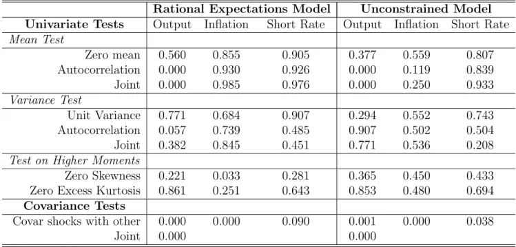
Appendix C describes the different specification tests that we perform on the residuals of the model. First, for each equation, we test the hypotheses of a zero mean and zero serial correlation (up to two lags) of the residuals (the “mean test”); unit mean and zero serial correlation (two lags) for the squared standardized residuals (the “variance test”); zero skewness, and appropriate kurtosis. In performing these tests, we recognize that the test statistics may be biased in small samples, especially if the data generating process is as non-linear as the model is above. Therefore, we use critical values from a small Monte Carlo analysis also described in Appendix C. Second, the economic model should also capture the correlation between the various variables. We test for each residual whether its joint covariances with all other residuals are indeed zero. We also perform a joint test for all covariances. As in the first set of tests, we obtain critical values from a small Monte Carlo analysis.

4_{We sacrifice full efficiency by ignoringf(X}f

t|It−1;θ) in the estimation. Technically, this requires assuming f(Xtf|St =st, It−1;θ) =f(Xtf|It−1;θ).While not very palatable at first, in our model, the regimes can in

Table 1 reports Monte Carlo p-values of all these tests for our main model, on the left hand side. The residual levels and variances are well behaved, with the exception of the output gap, where the test uncovers some remaining autocorrelation in the residuals. The regime-switching model is able to capture most skewness and kurtosis in the data, only failing the zero skewness test for inflation. The model’s weakest point appears to be the fit of covariances between the three shocks. The last two lines in Table 1 reveal that the model fails to fully capture the correlation structure between the various economic variables.

4

Empirical Results

4.1

Parameter estimates

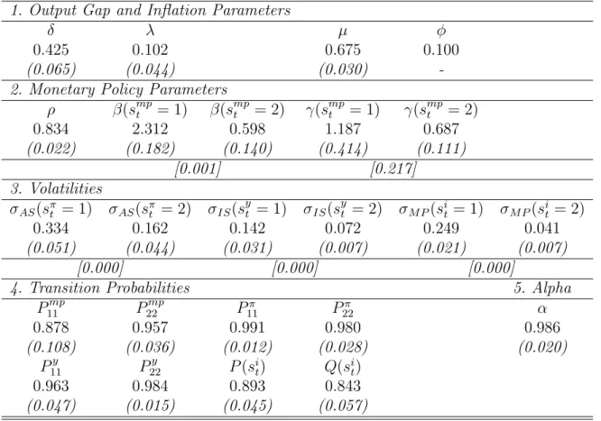
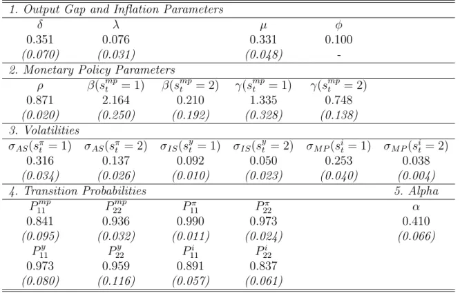
Table 2 presents the parameter estimates of the RS DSGE New-Keynesian macro model yielding a stable and determinate RE equilibrium, as described in Section 2.3. It also shows a number of statistical tests of parameter equality. All parameters have the right sign and are statistically significant, but we did constrain the φ coefficient to a positive value of 0.1. As is common in maximum likelihood estimation of this class of New-Keynesian models, unconstrained estimation yields either negative or very small and insignificant estimates of

φ (see Ireland (2001), Fuhrer and Rudebusch (2004) and Cho and Moreno (2006)).

In the AS equation, δ is 0.425, implying a similar weight on the forward-looking and endogenous persistence terms. The IS equation is more forward looking, since µ is 0.675. Given the small standard errors of these parameters, our estimation reveals strong evidence in favor of endogenous persistence.

The Phillips curve parameter λ is large at 0.102, implying a strong transmission mecha-nism from output to inflation and thus a strong monetary policy transmission mechamecha-nism. Previous estimations of rational expectations models fail to obtain reasonable and significant estimates ofλwith quarterly data (Fuhrer and Moore (1995)). Some alternative estimations have yielded significant estimates, such as Gal´ı and Gertler (1999) who use a measure for marginal cost replacing the output gap; Bekaert, Cho, and Moreno (2010) who identify a natural rate of output process from term structure data; or Roberts (1995) and Adam and Padula (2003) who use SBE but in a single equation context with fixed regimes. However, our estimate is even larger than the coefficients reported in these articles. We conjecture that the introduction of slow moving SBE of inflation generates additional correlation between (expected) inflation and the output gap.

agree-ment with most studies in the literature (Clarida, Gal´ı and Gertler (1999), Bekaert, Cho and Moreno (2010), among others). Our estimation allows for regime switches in the key monetary policy parameters, β, the response to expected inflation, and γ, the response to the output gap. In the “activist” regime, β is 2.312, well above 1 statistically, whereas in the passive regime,β is 0.598, significantly below 1. Thus, our estimation clearly identifies a sharp economic and statistical difference in the response to inflation across monetary policy regimes. In their single equation monetary policy rule estimation, Davig and Leeper (2005) also estimate a significant difference betweenβ’s across regimes, but of a smaller magnitude than our estimates. The contemporaneous articles of Bikbov and Chernov (2008) and Bianchi (2010), estimating Markov Switching RE New-Keynesian models, also identify a large differ-ence in β across regimes. The interest rate response to the output gap, γ, is higher than in the aforementioned estimations (1.187 and 0.687, respectively), and it is larger in the more “activist” regime, although not in a statistically significant way.

Finally, α, the parameter governing the law of motion for the survey-based expectations, is 0.986, meaning that SBE adjust almost completely to RE. We examine below whether this finding is the result of imposing rational expectations on the estimation. Because the other parameters are directly related to the identification of the regimes, we discuss them in the next sub-section.

4.2

Macroeconomic regimes

Perhaps the key output of our model is the identification of macroeconomic regimes. The volatility parameters imply strong evidence of time-varying variances in macroeconomic shocks. For the output gap and inflation shocks, volatility in the high volatility regime is around double that in the low volatility regime. However, for interest rates, the high volatil-ity regime features volatilvolatil-ity that is about 6 times as high as in quiet times, suggesting a potentially important role for discretionary monetary policy. Because interest rates are mea-sured in quarterly percent, the volatility of interest rate shocks in the low volatility state is very small (0.04%), implying a strict commitment to the monetary policy rule.

The transition probability coefficients imply overall quite persistent regimes. For inflation, the expected duration of the high variance regime is very high at 100 quarters, but the low variance regime is persistent as well. Output gap regimes are somewhat less persistent, with the high variance regime expected to last about 27 quarters, while discretionary interest rate regimes are much less persistent, with the high interest rate variability regime expected to last about 8 quarters. Accommodating monetary policy regimes last on average longer than

activist regimes, which are short-lived lasting on average 7 quarters.

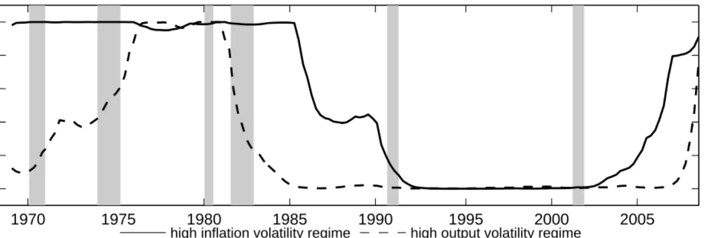
These transition probabilities are important inputs in the identification of the time path of the regimes. Figure 1 plots the smoothed probabilities for the four independent regime variables. Panel A shows the smoothed probabilities of respectively the high inflation shock volatility regime and the high output shock volatility regime. Note that the regime proba-bilities tend to be either close to one or zero, indicating adequate regime identification. We observe a sudden drop in output shock volatility starting in 1981 and fully materializing in 1985. The decreased volatility persists until 2007, coinciding with the onset of the credit crisis. The variability of inflation shocks starts to decrease later, with the smoothed proba-bility going below 0.5 at the beginning of 1986, and going toward zero just before the 1990 recession. Signs of a reversal in the low variability regime are already visible in 2003, with its probability reaching less than 50 percent in the third quarter of 2006 already. Our evidence in favor of a switch towards a higher variability regime is stronger and its timing earlier than in Bikbov and Chernov (2008).

Panel B shows the smoothed probabilities of respectively the active monetary policy regime in which the Fed aggressively stabilizes inflation, and the high volatility regime for interest rate shocks. The high interest rate volatility regime occurs quite frequently and is always on during recessions, including during the 1980-1982 Volcker period. This implies that in times of recession, the Fed is more willing to deviate from the interest rate rule. Bikbov and Chernov (2008) also categorize the Volcker period as a period of discretionary monetary policy. Unlike their results, we also find systematic monetary policy to be activist during this period. Interestingly, our model shows that activist monetary policy spells generally became more frequent from 1980 onwards. We identify the 1993-2000 period as an accommodating monetary policy stance. Because this period is characterized by relatively low inflation, a passive monetary policy stance implies relatively high interest rates. One interpretation is that inflation expectations were firmly anchored, due to the more aggressive stance of the Fed during the previous decade. In addition, the possibility of switching back to the stabilizing regime, as captured by our regime switching DSGE, may also anchor inflation expectations. Notice that this regime identification is quite different from the permanent shift in monetary policy around 1980, put forward in earlier studies such as Clarida, Gal´ı, and Gertler (1999) and Lubik and Schorfheide (2004), but consistent with contemporaneous results in Bianchi (2010) and Fern´andez-Villaverde, Guerr´on-Quintana, and Rubio-Ram´ırez (2010).

In 2000 there is a switch to the activist regime, as interest rates rapidly declined following the beginning of the 2000 recession, while inflation stayed low. Hence, according to our analysis, interest rates in the first 5 years of the previous decade were lower than what

was prescribed by the Taylor rule (see Taylor (2009)). Bernanke (2010) ascribes this to the “jobless recovery” experienced at the time, but some may surmise that this aggresive monetary policy was one of the root causes of the recent credit crisis (see Rajan (2006)). The recent credit crisis starting in 2007 is preceded by a passive monetary policy regime which, given the low inflation environment, implies that interest rates increased. In the beginning of the credit crunch, our model identifies a switch towards both systematic stabilizing and (expansionary) discretionary monetary policy, leading to a sharp decline of interest rates.

4.3

Impulse responses

A nice feature of our model is that the impulse responses are regime-dependent, and should differ across regimes. Because agents are assumed to know the regime, we compute the impulse responses using an information set that incorporates both data and the regime; they follow from calculatingE[Xt+k|It, smpt =i], fori= 1,2. Appendix D describes a simple

procedure to compute these impulse responses recursively. Note that this computation takes into account the expectations of agents regarding future switches in the monetary policy regime.

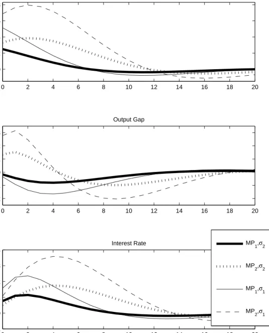
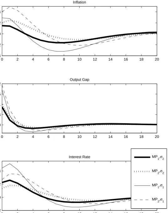
Figures 2 to 4 produce these regime dependent impulse responses of all three macro-variables to one-standard deviation shocks, focusing on, respectively, AS, IS and mone-tary policy shocks. In each figure, there are three panels corresponding to the three macro-variables. We show 4 different impulse responses, depending on the monetary policy regime and the shock volatility regime. While the volatility regimes only affect the initial size of the shock, the relative magnitude of the impulse responses helps us interpret macroeconomic dynamics in different time periods.

Figure 2 focuses on AS shocks. This is of considerable interest as there is a lively debate on whether the stagflations of the seventies were partially policy driven. The figure shows that following an AS shock, inflation is highest in the high volatility passive monetary pol-icy regime, as was observed in the 1970s, and lowest in the low volatility-activist monetary policy regime, as observed throughout the 90s. It is especially activist monetary policy that contributes to a lower inflation response. Investigating output gap responses, a positive AS shock drives down the output gap in a protracted way under an activist monetary policy response, because the real interest rate increases. However, the output gap increases when monetary policy is accommodating as then the real interest rate decreases following a positive AS shock. However, after about 6-7 quarters, the output gap is lower under an accommodat-ing regime than it is under an activist regime. The effect of AS shocks on nominal interest

rates is also strikingly regime-dependent. Except for the initial periods, the accommodating regime yields higher nominal interest rate responses than the activist regime. This is because under accommodating monetary policy, it takes time for inflation to decrease - both through the direct effect of monetary policy and through expectations -, so that interest rates must be kept high for a long time. The regime-dependent responses therefore provide simultane-ously an interesting interpretation of the historical record on the macroeconomic response to the negative aggregate supply shocks in the seventies and a counter-factual analysis. The accommodating policy regime implied (excessively) high interest rates, high inflation and high inflation variability and a substantial long term loss in output. The responses under an activist regime show that an aggressive Fed could have likely lowered the magnitude of the inflation response, reduced inflation volatility, kept interest rates overall lower and avoided the longer-term output loss, at the cost of a short-term loss over the first 5 quarters.

Figure 3 shows the responses to the IS shock. The inflation responses are similar across monetary policy regimes, but move over a wider range under the accommodating regime. In that regime, inflation rates move substantially below their mean during some periods, simultaneously with the interest rate undershooting its mean. The output gap responses are also quite similar across regimes. The similarity of the responses may have something to do with the fact that monetary policy reacts similarly to demand shocks across both regimes. While Panel C shows that the interest response to a demand shock is higher in the activist regime, the response differences are both in absolute and relative terms multiple times smaller than the responses to supply shocks, observed in Figure 2.

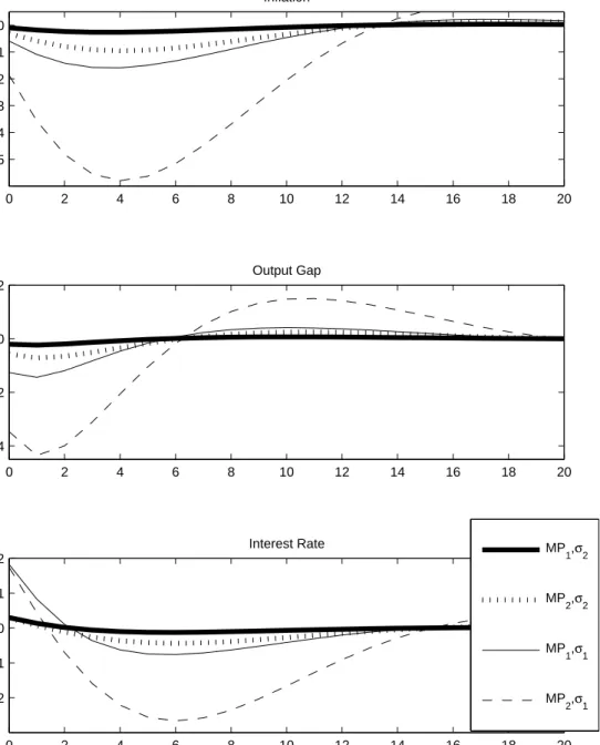
Finally, Figure 4 shows the responses to the monetary policy shock. Clearly, the activist monetary policy regime implies (much) more stable inflation and output dynamics than the passive regime. The macroeconomic volatility under the accommodating regime is especially dramatic when the interest rate shock is in the high volatility regime (recall that the interest rate shock volatility is multiple times higher in that case). A contractionary monetary policy shock lowers inflation and the output gap in both regimes, but, as the third panel shows, this is not only accommodated with less macroeconomic but also less interest rate volatility in the activist regime.

4.4

Macro-variability and its Sources

US economic history has witnessed profound changes in the volatility of macroeconomic variables over time, as evidenced by the literature on the Great Moderation. In the context of our model, this time variation in macroeconomic variability is driven by changing regimes in

the variability of macroeconomic shocks (driven bysπ

t, syt, sit) and regime dependent feedback

parameters, which also depend on the monetary policy regime, smp_t . In this section, we derive the unconditional and regime–dependent variances of our macro variables, and provide different decompositions to shed light on the sources of macroeconomic variability.

4.4.1 A Variance Decomposition

The regime variableStcontains 16 different regimes, as each of the four independent regimes, smp_t ,sπ

t, syt and sit has two states. Appendix E shows in detail how to compute the

uncondi-tional variance as a sum of regime-dependent variances:

V ar(Xt) = S

X

i=1

V ar(Xt|St =i)·Pi (17)

wherePi = Pr(St =i) is the unconditional, ergodic regime probability, andS = 16.Appendix

E also derives closed-form expressions for the regime-dependent variances. We then compute the contribution of a particular regime of a particular regime to the total variance as:

rx(St=i) =

V ar(xt|St=i)Pi V ar(xt)

(18) where xt represents πt, yt orit.

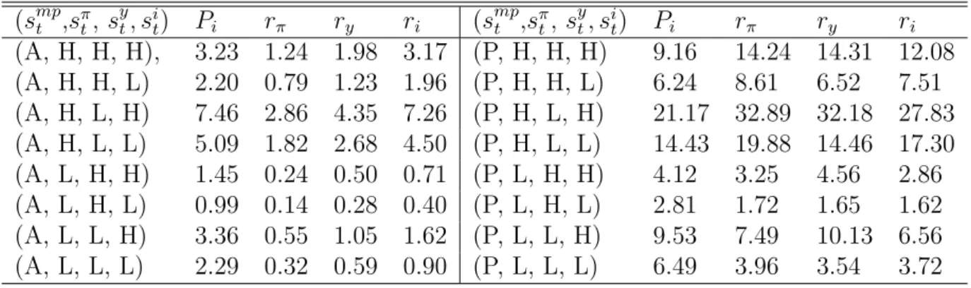
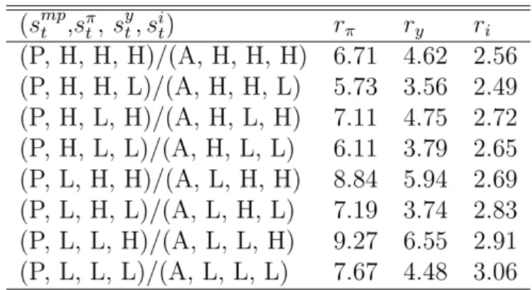
Table 3 reports these ratios together with the long run, ergodic distribution (Pi). For

instance, the regime combination of an active monetary policy and high shock volatility across all three equations contributes 1.24, 1.98 and 3.17% to the total variance of inflation, the output gap and the interest rate, respectively. The regimes contributing the most to the unconditional variance reflect passive monetary policy, the high variability regime for inflation shocks and the low variability regime for output shocks. The latter is true because the low variability regime for output occurs more frequently than the high variability regime (69.81% versus 30.19% in fact), whereas the opposite is true for inflation shocks, where the high variability regime occurs 68.97% of the time and also for interest rate shocks where the high variability regime occurs 59.47% of the time.

The most noticeable result is that in all cases, the contribution to total variance of any variable is much smaller under the active monetary regime than it is under the passive regime. For instance, when the economy is in the high volatility regime for all shocks, the active regime contributes only 1.98% to the total variance of the output gap, whereas the

passive regime contributes 14.31%, about 7.23 times more. Of course, the contribution could simply be low because the active regime has a much lower probability of occurring. In the high volatility regimes, the ergodic probability of the active regime is 3.23% while it is 9.16% under the passive regime, about three times higher. Therefore, even after controlling for differences in ergodic probatilities, the volatility of the output gap under the active regime is much smaller than that under the passive regime. This is generally true for all regime combinations and all the macro-variables.

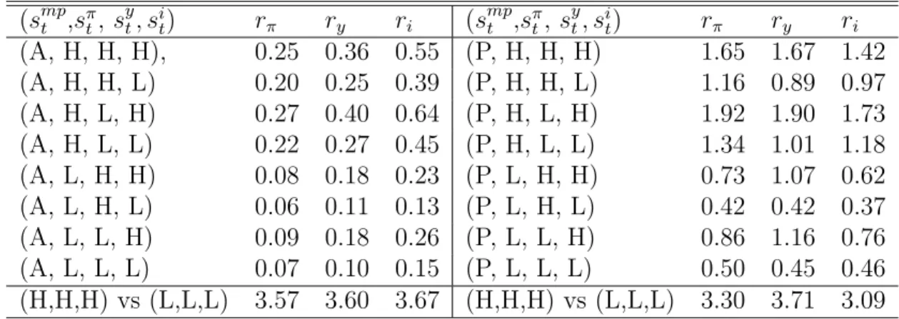
To see this more explicitly, Table 4 shows variance ratios for the various regimes, that is the variance in that particular regime relative to the unconditional variance. Strikingly, the variance ratios for output and inflation variability in the active regime when all the shocks are in the high variability regime is lower than the variance ratio for the output and inflation variability in the passive regime when all the shocks are in the low variability regime. This suggests that the monetary policy regime has a rather important impact on macro-variability and perhaps an impact that exceeds the impact of the variability of macro shocks.

To compare the relative effect on variability of shocks versus policy, the last line shows the ratio of the variance in a regime where all macro shocks are in the high variability regime versus the variance of a regime where all the macro shocks are in the low variability regime. These ratios obviously depend on the macro variable and the policy regime, but their range is rather narrow varying between 3.09 and 3.71. To compare this to the effect of monetary policy, Table 5 shows the ratio of the passive versus active variances, controlling for the shock variability regimes. It is obvious that policy has a relatively larger effect on output and inflation variances than do macro shocks. In terms of volatilities (standard deviations), the passive monetary policy regime leads to macro standard deviations that are about two to three times as large as macro standard deviations in the active regime.

4.4.2 The Great Moderation

The above computations can also help us identify the start and the end of the Great Mod-eration. In terms of our covariance stationary model, the Great Moderation is a period in which the regime-dependent variance is substantially below its unconditional counterpart. Figure 5 graphs the ratio of an estimate of the regime-dependent variance over time relative to the unconditional variance for inflation, the output gap and interest rates. To estimate regime dependent variances, we use the smoothed regime probabilities. That is,

V ar[Xt|IT] = S

X

i=1

If regime classification is perfect (that is, the smoothed probabilities are zero or 1), the summation simply selects one of the 16 regime-dependent variances. Visually, the graph clearly identifies the Great Moderation lasting from the third quarter of 1980 to the third quarter of 2004, with inflation and output variability being substantially below the 1 line, often even being less than 50% of the unconditional variance. Do note that there are short episodes during the Great Moderation where inflation and particularly output variability briefly spike up.

Our previous computations suggest that policy played a rather important role in the Great Moderation. For example, it is striking that we identify the Great Moderation to start before the shock variabilities move to a higher variability regime. This is, of course, due to a switch from a passive to active monetary policy regime around 1980. To visualize the effect of policy on macro-variances, we run a counterfactual analysis. In Figure 6, we graph a volatility ratio, namely the volatility of the three macro variables, conditional on the monetary policy regime always being in the passive regime versus the unconditional volatility. That is, when computing the counterfactual volatility, the underlying variances computation transfers mass from states where S_tmp = 1 to the corresponding state (and its variance) where S_tmp = 2. Figure 7 does the opposite computation, it computes the volatility assuming the monetary policy regime is always activist, and graphs the actual over the activist volatility.

With these two graphs in hand, we can reinterpret the historical evolution of macro-volatility as generated by our model. In the seventies, macro-macro-volatility was around twice as high as it could have been, had monetary policy been active (see Figure 7). From 1981 to 1993, active monetary policy managed to reduce macro-volatility substantially - it would have been 50% to 200% higher otherwise (Figure 6). The relatively subdued macro-variability after 1993 to around 2000 was due to low variability in the macro shocks, as monetary policy was passive. Of course, as we have argued before, the earlier aggressive policy stance may have helped anchor expectations during a rather mild macroeconomic climate. Taking our model literally, monetary policy could have further reduced macro-volatility by continuing to be aggressive. Because inflation was low at that time, an active monetary policy would have meantlower interest rates. The jump in counterfactual volatility around 2000 in Figure 6 is the more dramatic of the two graphs. In other words, if monetary policy had remained passive, macro-volatilities would have increased substantially. Bernanke’s (2010) speech ex-plicitly discusses this episode as the Federal Reserve reacting aggressively to a deflation scare, reducing the interest rate way below what a standard Taylor rule would predict. The period also witnessed a number of macroeconomic shocks that could have caused macro-volatility to increase and augmented recession risk, such as the events of September 11, 2001.

4.5

Robustness checks

To ensure that our results are robust, we consider a few alternative specifications. We sum-marize some major features of these alternative estimations in Table 6, repeating the main estimation results in the left column. The first two estimations we consider simply putφequal to a different number than the current value of 0.10, namely 0.01 and 0.20. The Phillips curve parameter,λ, remains large in both cases, and the stark contrast between the expected infla-tion response parameters in the active and passive monetary policy regimes is preserved. We also report the start and end of the Great Moderation for the variability of both output and inflation shocks under the various models. For output, the end of the low volatility regime is always in the first or second quarter of 2008, but the alternative estimations time the beginning of the low output shock volatility regime a bit later than our main estimation did. For inflation, using a smaller φ gives very similar results to the main estimation, but using

φ= 0.20 delays the start of the low volatility regime from the second quarter of 1986 to the second quarter of 1990, and speeds up its demise by three quarters (from the third quarter in 2006 to the last one in 2005). Do note that our cut-off for regime classification is 0.5: that is, as soon the shock volatility regime has a larger than 50% smoothed probability of being in either regime it is classified as being in that regime. However, when inflation transitions to a lower volatility regime, the regime probabilities in the models for φ= 0.10 andφ = 0.01 hover around 0.5 for a while, meaning that classification is uncertain. When we use a more stringent classification of the probability being in either regime being 70%, the start of the low inflation shock volatility regime is in early 1990 in all three cases. Finally, the last two rows report the probability of activist spells before and after 1980. For all three model spec-ifications we find no activist spells before 1980 and an elevated occurrence of activist spells post 1980.

The second set of columns report the three previous estimations but making γ regime invariant. The results are very robust, with the remarks about the start of the Great Mod-eration for inflation shocks being the same as before.

4.6

Rational expectations versus survey expectations

Our estimation imposes a parameter space that ensures the existence of a fundamental rational expectations equilibrium. What happens if this assumption is relaxed? Table 7 shows the results for the unconstrained estimation. In Table 1, the right-hand side panel also produces specification tests for this model. The model only performs marginally better than the constrained model. Moreover, the resulting estimates imply explosive dynamics for

the RE model. Nevertheless, it is noteworthy that the parameter estimates are very similar to those obtained in the constrained estimation. The only significant difference is thatµ, the forward-looking parameter in the IS equation, is now significantly smaller, 0.331, relative to 0.675 before. This is similar to the values obtained by Fuhrer and Rudebusch (2004), in their systematic single equation estimation in a fixed regime context. Bekaert, Cho, and Moreno (2010) also estimate a lower value for µ, namely 0.422, but this is coupled with a high estimate for the degree of forward-looking behavior in the AS equation (δ in our model). As we have verified through simulation exercises, the combination of lowδ and low

µ–maintaining standard values for other parameters - implies the non-existence of a stable RE equilibrium, both in a fixed regime and in a multiple regime context. In economic terms, stable RE dynamics require AS and IS equations with a sufficient degree of forward looking behavior, such that shocks are rapidly absorbed.

Finally, α, the parameter governing the law of motion for the survey-based expectations, is 0.410 in the unconstrained case, whereas it was 0.986 in the constrained estimation. This is an important difference. When we enforce a stable RE, RE appear indistinguishable from SBE, whereas in the unconstrained estimation, SBE slowly adjust to RE, being heavily influenced by past expectations. In fact, α is statistically indistinguishable from 0.5, im-plying that rational expectations and past survey-based expectations obtain similar relative weigths in the expectations formation process. In other words, viewed through the lens of this macroeconomic model, survey expectations only slowly adjust to rational expectations, being heavily influenced by past expectations. This is consistent with Mankiw, Reis, and Wolfers (2003), who show that the adjustment of SBE to the macro environment is grad-ual. Conversely, the dependence on rational expectations is highly significant, implying that survey expectations likely convey much information, useful in estimating macroeconomic parameters and dynamics.

Figure 8 shows the regime probabilities for the unconstrained model, which should be compared to Figure 1 for the RE model. Focusing first on Panel B, the monetary policy regime identification, both for systematic and discretionary policy is very similar, qualitatively and quantitatively, to that in the constrained estimation. In Panel A, we observe some differences in terms of output shock regime identification. First, the high output volatility prevails from the beginning of the sample, whereas in the unconstrained estimation this regime appears more gradually. In addition, the Great Moderation in terms of output volatility shocks starts abruptly around 1986, which is a few years later than in the constrained estimation. Second, the low volatility output shock regime already ends in 2000, much earlier than in the constrained optimization. These differences can be easily understood examining the transition probabilities of the IS shock regime variable across estimations (see Tables

2 and 6). The unconstrained estimation shows much more persistence in the high variance regime and less persistence in the low volatility regime than the constained estimation.

5

Conclusions

In this article, we indentified macroeconomic regimes through the lens of a simple New-Keynesian model accommodating regime switches in macroeconomic shocks and systematic monetary policy. We demonstrate that monetary policy has witnessed several spells of activist policy, which have become more frequent post 1980. Nevertheless, we do not see a permanant switch from accommodating to activist policy around 1980, but rather occasional switches back and forth between the two regimes. One reason is that the data suggest an important and time-varying role for discretionary monetary policy. For example, the Volcker period is characterized by both activist systematic policy and discretionary active policy. We also document important changes in the variances of output and volatility shocks. It is no surprise that we find strong evidence of a “shock variability moderation” occuring around 1985 for output, whereas for inflation the timing is somewhere between 1985 and 1990. What is new is that we find strong evidence of this volatility reduction having ended, for output at the onset of the recent economic crisis (more precisely in 2007), for inflation, earlier in 2005. The variability of shocks is not the only determinant of macro-variability however. Our model implies that the effect of monetary policy regimes on macro variability is relatively larger than the effect of the variability of shocks. When we investigate the time path of the overall variability of inflation and the output gap, we find that the Great Moderation starts around 1980 and ends in about 2005. During that period, a predominantly active monetary policy and low variability economic shocks combined to make output and inflation substantially less variable than unconditional averages would suggest.

Estimating a rational expectations New-Keynesian model with regime switches is very difficult from a numerical perspective. Our innovation was to expand the information set with survey expectations on inflation and output growth. By formulating a simple law of motion for these expectations as a function of the true rational expectations, we could greatly simplify the likelihood construction. Constraining the parameter space to those parameters that yield a stable rational expectations equilibrium, we find survey expectations to be almost equivalent to rational expectations. However, when we relax these constraints, we find survey expectations to only gradually adjust to rational expectations and the parameters to be outside the rational expectations equilibrium space. Fortunately, the identification of regimes remains similar to that obtained in the rational expectations model, except that the

Great Moderation in terms of output volatility ends much earlier (in 2000!) when identified from the unconstrained model.

There are two possible interpretations to these different estimation results. One possi-bility is that agents truly have rational expectations but that our New-Keynesian model is mis-specified. Perhaps, we need a more intricate natural rate of output process or we must add investment equations as in Smets and Wouters (2007) to better fit the data. We did experiment with slightly more complex specifications (e.g. three monetary policy regimes, state-dependent transition probabilities, correlated regimes) within the confines of the styl-ized New-Keynesian model, finding little improvement in fit, and no noteworthy new results. Perhaps some of the parameters we now assume to be time-invariant may also be unsta-ble. Hofmann, Peersman, and Straub (2010), for instance, indicate that the degree of wage indexation may vary through time, causing instability in the AS equation. An alternative possibility is that the assumption of rational expectations is too rigid, and we must build a model that accommodates the presence of agents with not fully rational expectations. In any case, we hope this article stimulates the use of survey expectations in building and estimating macroeconomic models.

References

Adam, K., and M. Padula, 2003, “Inflation Dynamics and Subjective Expectations in the United States,”ECB Working Paper, No. 222.

Ang, A., G. Bekaert, and M. Wei, 2007, “Do Macro Variables, Asset Markets or Surveys Forecast Inflation Better?,”Journal of Monetary Economics, 54, 1163–1212.

Ang, A., G. Bekaert, and M. Wei, 2008, “The term structure of real rates and expected inflation,”The Journal of Finance, 63(2), 797–849.

Ang, A., J. Boivin, S. Dong, and R. Loo-Kung, 2010, “Monetary Policy Shifts and the Term Structure,”Review of Economic Studies, Forthcoming.

Bekaert, G., S. Cho, and A. Moreno, 2010, “New-Keynesian Macroeconomics and the Term Structure,”Journal of Money, Credit, and Banking, 42(1), 33–62.

Benati, L., and P. Surico, 2009, “VAR Analysis and the Great Moderation,” American Eco-nomic Review, 99, 1636–52.

Bernanke, B., 2010, “Monetary Policy and the Housing Bubble,”Speech at the Annual Meet-ing of the American Economic Association, Atlanta (Georgia).

Bianchi, F., 2010, “Regime Switches, Agent’s Beliefs, and Post-World War II U.S.,” Duke University Working Paper.

Bikbov, R., and M. Chernov, 2008, “Monetary Policy Regimes and The Term Structure of Interest Rates,” Working Paper, Columbia University.

Blanchard, O., and J. Simon, 2001, “The long and large decline in US output volatility,” Brookings Papers on Economic Activity, (1), 135–174.

Boivin, J., 2006, “Has US Monetary Policy Changed? Evidence from Drifting Coefficients and Real-Time Data,”Journal of Money, Credit and Banking, 38(5), 1149–1173.

Boivin, J., and M. P. Giannoni, 2006, “Has Monetary Policy Become More Effective?,” Review of Economics and Statistics, 88(3), 445–462.

, 2008, “Optimal Monetary Policy in a Data-Rich Environment,”Working Paper. Cho, S., 2010, “Characterizing Markov-Switching Rational Expectations Models,” Working