Improving Naïve Bayes classifier using conditional probabilities paper
presented at Conferences in Research and Practice in Information
Technology Series, Ballarat, 2010
Copyright Australian Computer Society, Inc
COPYRIGHT NOTICE
UB ResearchOnline
Improving Naive Bayes Classifier
Using Conditional Probabilities
SONA TAHERI
1MUSA MAMMADOV
1,2ADIL M. BAGIROV
11Centre for Informatics and Applied Optimization, School of Science, Information Technology and Engineering, University of Ballarat, Victoria 3353, Australia
2 National Information and Communications Technology Australia (NICTA) Emails: [email protected],
[email protected], [email protected]
Abstract
Naive Bayes classifier is the simplest among Bayesian Network classifiers. It has shown to be very efficient on a variety of data classification problems. However, the strong assumption that all features are condition-ally independent given the class is often violated on many real world applications. Therefore, improve-ment of the Naive Bayes classifier by alleviating the feature independence assumption has attracted much attention. In this paper, we develop a new version of the Naive Bayes classifier without assuming inde-pendence of features. The proposed algorithm ap-proximates the interactions between features by using conditional probabilities. We present results of nu-merical experiments on several real world data sets, where continuous features are discretized by apply-ing two different methods. These results demonstrate that the proposed algorithm significantly improve the performance of the Naive Bayes classifier, yet at the same time maintains its robustness.
Keywords: Bayesian Networks, Naive Bayes, Semi Naive Bayes, Correlation
1 Introduction
Classification is the task to identify the class labels for instances based on a set of features, that is, a function that assigns a class label to instances de-scribed by a set of features. Learning accurate clas-sifiers from pre classified data is an important re-search topic in machine learning and data mining. One of the most effective classifiers is Bayesian Net-works (Shafer 1990, Heckerman 1995, Jensen 1996, Pearl 1996, Castillo 1997). A Bayesian Network (BN) is composed of a network structure and its conditional probabilities. The structure is a directed acyclic graph where the nodes correspond to domain vari-ables and the arcs between nodes represent direct de-pendencies between the variables. Considering an in-stance X = (X1, X2, ..., Xn) and a class C, the clas-sifier represented by BN is defined as
arg max c∈C P(c|x1, x2, ..., xn)∝arg max c∈C P(c)P(x1, x2, ..., xn|c), (1) where xi, care the values of Xi, C respectively.
Copyright c2011, Australian Computer Society, Inc. This pa-per appeared at the 9th Australasian Data Mining Conference (AusDM 2011), Ballarat, Australia, December 2011. Confer-ences in Research and Practice in Information Technology (CR-PIT), Vol. 121, Peter Vamplew, Andrew Stranieri, Kok-Leong Ong, Peter Christen and Paul Kennedy, Ed. Reproduction for academic, not-for-profit purposes permitted provided this text is included.
However, accurate estimation ofP(x1, x2, ..., xn|c) is non trivial. It has been proved that learning an op-timal BN is NP-hard problem (Chickering 1996, Heck-erman 2004). In order to avoid the intractable com-plexity for learning BN, the Naive Bayes classifier has been used. In the Naive Bayes (NB) (Langley 1992, Domingos 1997), features are conditionally indepen-dent given the class. The simplicity of the NB has led to its wide use, and to many attempts to extend it (Domingos 1997). Since NB assumes the strong assumption of independency between features, learn-ing semi Naive Bayes has attracted much attention from researchers (Langley 1994, Kohavi 1996, Paz-zani 1996, Friedman 1997, Kittler 1986, Zheng 2000, Webb 2005). The semi Naive Bayes classifiers are based on the structure of NB, requiring that the class variable be a parent of every feature. However, they allow additional edges between features that capture correlation among them. The main aim in this area of research has involved maximizing the accuracy of classifier predictions.
In this paper, we propose a new version of the Naive Bayes classifier (semi Naive Bayes) without as-suming independence of features. The proposed algo-rithm finds dependencies between features using con-ditional probabilities. This algorithm is a new al-gorithm and different from the existing semi Naive Bayes methods (Langley 1994, Kohavi 1996, Pazzani 1996, Friedman 1997, Kittler 1986, Zheng 2000, Webb 2005).
Most of data sets in real world applications often involve continuous features. Therefore, continuous features are usually discretized (Lu 2006, Wang 2009, Ying 2009, Yatsko 2010). The main reason is that the classification with discretization tend to achieve lower error than the original one (Dougherty 1995). We apply two different methods to discretize continu-ous features. The first one, which is also the simplest one, transforms the values of features to{0,1} using their mean values. We also apply the discretization algorithm using sub-optimal agglomerative clustering algorithm from (Yatsko 2010) which allows us to get more than two values for discretized features. This leads to the design of a classifier with higher testing accuracy in most data sets used in this paper.
We organize the rest of the paper as follows. We give a brief review to the Naive Bayes and some semi Naive Bayes classifiers in Section 2. In Section 3, we present the proposed algorithm. Section 4 presents an overview of the discretization algorithm using sub-optimal agglomerative clustering. The numerical ex-periments are given in Section 5. Section 6 concludes the paper.
2 Naive Bayes and Semi Naive Bayes Classi-fiers
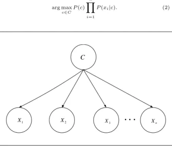
The Naive Bayes (NB) assumes that the features are independent given the class, it means that all features have only the class as a parent (Kononenko 1990, Lan-gley 1992, Domingos 1997, Mitchell 1997). A sample of the NB withnfeatures is depicted in Figure 1. The NB, classifies an instanceX = (X1, X2, ..., Xn) using Bayes rule, by selecting
arg max c∈C P(c) n Y i=1 P(xi|c). (2) C 1 X X2 X3 Xn
Figure 1: Naive Bayes
NB has been used as an effective classifier for many years. Unlike many other classifiers, it is easy to con-struct, as the structure is given a priori. Although the independence assumption is obviously problem-atic, NB has surprisingly outperformed many sophis-ticated classifiers, especially where the features are not strongly correlated (Domingos 1997). In spite of NB’s simplicity, the strong independency assumption harms the classification performance of NB when it is violated. On the other hand, learning BN requires searching the space of all possible combinations of edges which is NP-hard problem (Chickering 1996, Heckerman 2004).
In order to relax the independence assumption of NB, a lot of effort has focussed on improving NB. The improved NB classifiers use exhaustive search to join features based on statistical methods. There are some improved algorithms of the NB. Langley and Sage (Langley 1994) considered Backwards Sequen-tial Elimination (BSE) and Forward SequenSequen-tial Se-lection (FSS) in which their methods select a subset of features using leave-one-out cross validation error as a selection criterion and establish a NB with these features. Starting from the full set of features, BSE successively eliminates the features whose elimination most improves accuracy, until there is no further ac-curacy improvement. FSS uses the reverse search di-rection, that is iteratively adding the features whose addition most improves accuracy, starting with the empty set of features. The work of Pazzani (Paz-zani 1996) introduces Backward Sequential Elimina-tion and Joining (BSEJ). It uses predictive accuracy as a merging criterion to create new Cartesian prod-uct features. The value set of a new compound fea-tures is the Cartesian product of the value sets of the two original features. As well as joining features, BSEJ also considers deleting features. BSEJ repeat-edly joins the pair of features or deletes the features
that most improves predictive accuracy using leave-one-out cross validation. This process terminates if there is no accuracy improvement. Kohavi (Kohavi 1996) proposed the NB Tree, a strategy that is a hy-brid approach combining NB and decision tree learn-ing. It partitions the training data using a tree struc-ture and establishes a local NB in each leaf. It uses 5-fold cross validation accuracy estimate as the split-ting criterion. A split is defined to be significant if the relative error reduction is greater than 5 percent and the splitting node has at least 30 instances. When there is no significant improvement, NB Tree stops the growth of the tree. As the number of splitting features is greater than or equals one, NB Tree is an x-dependence classifier. The classical decision tree predicts the same class for all the instances that reach a leaf. In NB Tree, these instances are classified us-ing a local NB in the leaf, which only considers those non tested features. Friedman et al. (Friedman 1997) introduced Tree Augment Naive Bayes (TAN) based on tree structure. It approximates the interactions between features by using a tree structure imposed on the NB structure. In TAN, each feature has the class and at most one other feature as parents. Super Parent algorithm is proposed by Keogh and Pazzani (Keogh 1999). This algorithm uses the same represen-tation as the Tree Augment Naive Bayes, but utilizes leave-one-out cross validation error as a criterion to add a link. The Super Parent is the feature that is the parent of all the other orphans, the features with-out a non-class parent. There are two steps to add a link: first selecting the best Super Parent that im-proves accuracy the most, and then selecting the best child of the Super Parent from orphans. This method stops adding links when there is no accuracy improve-ment. Zheng and Webb (Zheng 2000) developed Lazy Bayesian Rules (LBR), which adopts a lazy approach, and generates a new Bayesian rule for each test exam-ple. The antecedent of a Bayesian rule is a conjunc-tion of feature-value pairs, and the consequent of the rule is a local NB, which uses those features that do not appear in the antecedent to classify. LBR stops adding feature value pairs into the antecedent if the outcome of a one tailed pairwise sign test of error dif-ference is not better than 0.05. As the number of the feature value pairs in the antecedent is greater than or equals one, LBR is anx-dependence classifier. Webb et al. (Webb 2005) proposed Averaged One Depen-dence Estimators (AODE), which averages the pre-dictions of all qualified 1-dependence classifiers. In each 1-dependence classifier, all features depend on the class and a single feature.
In the next section, we introduce a new version of the Naive Bayes classifier (semi Naive Bayes) with-out assuming independence of features. The proposed algorithm approximates the interactions between fea-tures by using conditional probabilities.
3 The Proposed Algorithm
In this section, we present a new algorithm that main-tains the basic structure of the NB, and thus ensure that the class C is the parent of all features. The proposed algorithm, however, removes the strong as-sumption of independence in the NB by finding corre-lation between features, while also capturing much of the computational efficiency of the NB. In this algo-rithm, the class has no parents and each feature has the class and at most one other feature as parents. Therefore, each feature can have one augmenting edge pointing to it. The procedure for learning these edges is based on the Pearson’s correlation and conditional
probabilities. First, we construct a basic structure of the NB with n features X1, X2, ..., Xn from the set
X and the classC. After that, we find the Pearson’s correlations between each feature Xi and the class
C using the formula (3), Corr(Xi, C). Then we re-order the setX as a setX∗ in a descending order of |Corr(Xi, C)|. In the ordered setX∗, an arc from the first feature is added to the second one. Finally, for all remain features, we find the conditional probabil-ities of each feature with the previous features given the class values in the ordered set X∗, formula (4). The highest value of these conditional probabilities between features is used to recognize the parent of each feature. The conditional probabilities described in (4), first introduced by Quinn et al. (Quinn 2009) and called influence weights, have been used directly for data classification. However, here, we used them for finding the dependencies between features.
The correlation coefficient (Graham 2008) between two random variables Xi andXj is defined as :
Corr(Xi, Xj) = N N P i,j=1 XiXj− N P i=1 Xi N P j=1 Xj s (N N P i=1 X2 i−( N P i=1 Xi)2)(N N P j=1 X2 j −( N P j=1 Xj)2) , (3) whereN is the number of data points. This measure has the property of |Corr(Xi, Xj)| ≤ 1. When this value is close to 1, it denotes the perfect linear cor-relation between Xi and Xj, and Corr(Xi, Xj) = 0 stands for no linear correlation.
The proposed algorithm consists of six main steps:
Algorithm. Proposed Algorithm
Step 1. Construct a basic structure of the Naive Bayes withnfeatures,
X={X1, X2, ..., Xn}, and the classC. Step 2. Compute the correlation between each featureXi, i= 1, ..., nand the classC using the formula (3),Corr(Xi, C).
Step 3. ReorderX as a set
X∗={X1∗, X2∗, ..., Xn∗}in a descending order of|Corr(Xi, C)|, i= 1, ..., n.
Step 4. Add an arc fromX1∗ toX2∗.
Step 5. Forj= 3, ..., n:
5.1 FindXi∗that has the highest value of
N
X
k=1
|P(X∗ki, X∗kj|C)−P(Xki∗, Xkj∗|C)|, i < j, (4)
whereXi∗= (X1∗i, X2∗i, ..., XN i∗ )T,N is the number of instances andC=−C.
5.2 Add an arc fromXi∗ toXj∗.
Step 6. Compute the conditional probability tables inferred by the new structure.
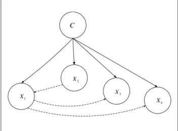
Figure 2 shows the structure of Svmguide1 data set, taken from LIBSVM, with four features (see Ta-ble 1) using the proposed algorithm. The solid lines are those edges required by the Naive Bayes classi-fier. The dashed lines are correlation edges between features found by our algorithm.
C 1 X 2 X 3 X 4 X
Figure 2: Proposed algorithm, Svmguide1
4 Discretization Algorithm Using
Sub-Optimal Agglomerative Clustering
(SOAC)
Discretization is a process which transform continu-ous numeric values into discrete ones. In this paper, we apply two different methods to discretize continu-ous features. The first one, which is also the simplest one, transforms the values of features to 0,1 using their mean values. We also apply the discretization algorithm using sub-optimal agglomerative clustering algorithm which allows us to get more than two values for discretized features. In this section, we introduce discretization algorithm SOAC which is an efficient discretization method for the NB learning. Details of this algorithm can be found in (Yatsko 2010).
Consider a finite set of points A in the n di-mensional space Rn, that is A = {a1, ..., am},
where ai ∈ Rn, i = 1, ..., m. Assume that the sets
Aj, j = 1, ..., k be clusters, and each clusterAj can be identified by its centroid xj ∈ Rn, j = 1, ..., k.
The discretization algorithm SOAC proceeds as follows.
Algorithm. Discretization Algorithm SOAC
Step 1. Setk=m,and a small value of parameterθ,0< θ <1. Sort values of the current feature in the ascending order. Each feature requiring discretization is treated in turn.
Step 2. Calculate the center of each cluster:
xj= X
a∈Aj
a
|Aj|, j= 1, ..., k
and the errorEk of the cluster system approximating setA: Ek= k X j=1 X a∈Aj kxj−ak2.
Step 3. Merge in turn each cluster with the next tentatively. Calculate the error increase after each mergeEk−1−Ek and choose the pair of clusters giving the least increase. Merge these two clusters permanently. Set
Step 4. Once the error of the current cluster sys-tem is over the set fraction of the maximum error corresponding to the single cluster Ek ≥ θE1 stop, otherwise go to Step 2.
5 Numerical Experiments
To verify the efficiency of the proposed algorithm, nu-merical experiments with a number of real world data sets have been carried out. We use 10 real world data sets. The detailed description of the data sets used in this experiments can be found in the UCI machine learning repository, with the exception of “Fourclass”, “Svmguide1” and “Svmguide3”. These three data sets are downloadable on tools page of LIBSVM. A brief description of data sets is given in Table 1. We discritize the values of features in data sets using two different methods. In the first one, we apply a mean value of each feature variable to discritize the values to{0,1}. The second one is the discrization algorithm SOAC (Yatsko 2010) which is presented in Section 4. We conduct empirical comparison for the NB and the proposed algorithm in terms of test set accuracy using two different discritization methods. The re-sults of the NB and the new algorithm on each data set were obtained via 1 run of 10-fold cross valida-tion. Runs were carried out on the same training sets and evaluated on the same test sets. In particular, the cross validation folds were the same for all exper-iments on each data set.
The test set accuracy obtained by the NB and the proposed algorithm on 10 data sets using mean values for discretization summarized in Table 2. The results presented in this table demonstrate that the test set accuracy of the new algorithm is much better than that of the NB. The proposed algorithm works well in that it yields good classifier compared to the NB. Its performance was further improved by introducing some additional edges in the NB, using conditional probabilities. Improvement is noticed mainly in large data sets. In 8 cases out of 10, the new algorithm has higher accuracy than the NB. The accuracy of this algorithm is same with the NB in data sets Fourclass and Svmguide1.
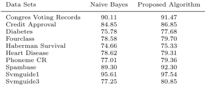
Table 3 presents the test set accuracy obtained by the NB and the proposed algorithm on 10 data sets using discretization algorithm SOAC. The results from this table show that the accuracy obtained by the new algorithm in all data sets are higher than those obtained by the NB.
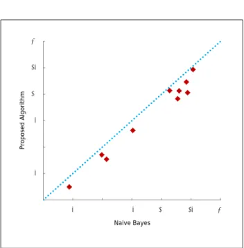
Figures 3 to 4 show the scatter plot comparing the proposed algorithm with the NB, using two different discritization methods. In these plots, each point rep-resents a data set, where thexcoordinate of a point is the percentage of miss classifications according to the NB and the y coordinate is the percentage of miss classification according the proposed algorithm. Therefore, points above the diagonal line correspond to data sets where the NB performs better, and points below the diagonal line correspond to data sets where the proposed algorithm performs better.
According to the results explained above, the pro-posed algorithm outperforms the NB, yet at the same time maintains its robustness. However, the proposed algorithm requires more computational effort than the NB since we need to compute conditional prob-abilities between features to recognize the parent of each feature in our algorithm.
Table 1: A brief description of data sets Data sets # Features # Instances
Congres Voting Records 16 435 Credit Approval 14 690 Diabetes 8 768 Fourclass 2 862 Haberman Survival 3 306 Heart Disease 13 270 Phoneme CR 5 5404 Spambase 57 4601 Svmguide1 4 7089 Svmguide3 21 1284
Table 2: Test set accuracy of NB and the proposed algorithm using mean value for discretization
Data Sets Naive Bayes Proposed Algorithm
Congres Voting Records 90.11 91.47 Credit Approval 84.85 86.85 Diabetes 75.78 77.68 Fourclass 76.82 76.82 Haberman Survival 74.51 75.66 Heart Disease 84.14 85.18 Phoneme CR 75.96 78.30 Spambase 90.13 93.45 Svmguide1 92.17 92.17 Svmguide3 80.61 87.18
Table 3: Test set accuracy of NB and the proposed algorithm using discretization algorithm SOAC
Data Sets Naive Bayes Proposed Algorithm
Congres Voting Records 90.11 91.47 Credit Approval 84.85 86.85 Diabetes 75.78 77.68 Fourclass 78.58 79.70 Haberman Survival 74.66 75.33 Heart Disease 78.62 79.31 Phoneme CR 77.01 79.36 Spambase 89.30 92.30 Svmguide1 95.61 97.54 Svmguide3 77.25 80.85 6 Conclusion
In this paper, we have developed the new version of the Naive Bayes classifier without assuming indepen-dence of features. An important step in this algorithm is adding edges between features that capture correla-tion among them. The proposed algorithm finds de-pendencies between features using conditional prob-abilities. We have presented the results of numeri-cal experiments on 10 data sets from UCI machine learning repository and LIBSVM. The values of fea-tures in data sets are discritized by using mean value of each feature and applying discretization algorithm SOAC. We have presented results of numerical exper-iments. These results clearly demonstrate that the proposed algorithm significantly improve the perfor-mance of the Naive Bayes classifier, yet at the same time maintains its robustness. Furthermore, this im-provement becomes even more substantial as the size of the data sets increases.
7 References References
Castillo, E., Gutierrez, J.M & Hadi, A.S. (1997), Ex-pert Systems and Probabilistic Network Models, Springer Verlag, New York.
Chang, C., & Lin, C. (2001), A library for support vector machines, Software available at http://www.csie.ntu.edu.tw/cjlin/libsvm.
Charniak, E. (1991), E. Bayesian Networks Without Tears. AI Magazine, 12 (4).
Chickering, D.M. (1996), Learning Bayesian Net-works is NP-complete. In: Fisher, D., Lenz, H. Learning from data: Artificial Intelligence and statistics V, Springer, pp. 121–130.
Domingos, P., & Pazzani, M. (1997), On the optimal-ity of the simple Bayesian classifier under zero-one loss. Mach Learn 29, pp. 103–130.
Dougherty, J., Kohavi, R., & Sahami, M., (1995), Su-pervised and unsuSu-pervised discretization of contin-uous features. In Proceedings of the 12th Interna-tional Conference on Machine Learning, pp. 194– 202.
Friedman, N., Geiger, D., & Goldszmidt, M. (1997), Bayesian network classifiers. Machine Learning 29 , pp. 131–163.
Graham, E., (2008), CIMA Official Learning System Fundamentals of Business Maths. Burlington : El-sevier Science and Technology.
Heckerman, D., Geiger, D., & Chickering, D.M. (1995), Learning Bayesian Networks: the Combi-nation of Knowledge and Statistical Data. Machine Learning, 20, pp. 197–243.
Heckerman, D., Chickering, D.M., & Meek.C. (2004), Large-Sample Learning of Bayesian Networks is NP-Hard. Journal of Machine Learning Research, pp. 1287–1330.
Jensen, F. (1996), An Introduction to Bayesian Net-works. Springer, New York.
Kohavi, R. (1996), Scaling up the accuracy of naive-Bayes classifiers: a decision-tree hybrid. In: Proc. 2nd ACM SIGKDD Int. Conf. Knowledge Discov-ery and Data Mining, pp. 202–207.
Keogh, E.J., & Pazzani, M.J., (1999), Learning augmented Bayesian classifers: A comparison of distribution-based and classification-based ap-proaches. In: Proc. Int. Workshop on Artificial In-telligence and Statistics, pp. 225–230.
Kittler, J. (1986), Feature selection and extraction. In Young, T.Y., Fu, K.S., eds.: Handbook of Pat-tern Recognition and Image Processing. Academic Press, New York.
Kononenko, I. (1990), Comparison of Inductive and Naive Bayesian Learning Approaches to Autpmatic Knowledge Acquisition. In Wielinga, B., Boose, J., B.Gaines, Schreiber, G., van Someren, M., eds. Current Trends in Knowledge Acquisition. Amster-dam: IOS Press.
Langley, P., Iba, W., & Thompson, K. (1992), An Analysis of Bayesian Classifiers. In 10th Inter-national Conference Artificial Intelligence, AAAI Press and MIT Presspp, pp. 223–228.
Langley, P., & Saga, S. (1994), Induction of selective Bayesian classifiers. In: Proc. Tenth Conf. Uncer-tainty in Artificial Intelligence, Morgan Kaufmann , pp. 399–406.
Lu, J., Yang, Y., & Webb, G. I. (2006), Incremental Discretization for Naive-Bayes Classifier, Springer, Heidelberg, vol. 4093, pp. 223–238.
Mitchell, T.M. (1997), Machine Learning. McGraw-Hill, New York.
Pazzani, M.J. (1996), Constructive induction of Cartesian product attributes. ISIS: In- formation, Statistics and Induction in Science, pp. 66–77. Pearl, J. (1988), Probabilistic Reasoning in Intelligent
Systems: Networks of Plausible Inference. Morgan Kaufmann.
Quinn, A., Stranieri, A., Yearwood, J., & Hafen, G. (2009), A classification algorithm that derives weighted sum scores for insight into disease, Proc. of 3rd Australasian Workshop on Health Informat-ics and Knowledge Management, Wellington, New Zealand.
Shafer, G., & Pearl, J. (1990), Readings in Uncertain Reasoning. Morgan Kaufmann, San Mateo, CA. Wang, S, Min, Z., Cao, T., Boughton, J., & Wang,
Z. (2009), OFFD: Optimal Flexible Frequency Dis-cretization for Naive Bayes Classification, Springer, Heidelberg, pp. 704–712.
Webb, G.I, Boughton, J., & Wang, Z. (2005), Not so naive Bayes: Aggregating one- dependence estima-tors. Machine Learning 58, pp. 5–24.
Yatsko, A., Bagirov, A. M., & Stranieri, A. (2010), On the Discretization of Continu-ous Features for Classification. School of Information Technology and Mathematical Sciences, University of Ballarat Conference, http://researchonline.ballarat.edu.au:8080/vital/ access/manager/Repository.
Ying, Y., & Geoffrey, I., (2009), Discretization For Naive-Bayes Learning: Managing Discretization Bias And Variance, In Machine Learning, 74(1): pp. 39–74.
Ying, Y., (2009), Discretization for Naive-Bayes Learning, PhD thesis, school of Computer Science and Software Engineering of Monash University. Zheng, Z., & Webb, G.I. (2000), Lazy learning of
Bayesian rules. Machine Learning 41, pp. 53–84. UCI repositary of machine learning databases
15 20 25 30 opo se d Al g orit h m 0 5 10 15 20 25 30 0 5 10 15 20 25 30 Pr op os ed A lgo ri th m Naive Bayes
Figure 3: Scatter plot comparing miss classifications of the proposed algorithm (y coordinate) with Naive Bayes (xcoordinate); using mean value for discritiza-tion 15 20 25 30 opo se d Al g orit h m 0 5 10 15 20 25 30 0 5 10 15 20 25 30 Pr op os ed A lgo ri th m Naive Bayes
Figure 4: Scatter plot comparing miss classifications of the proposed algorithm (y coordinate) with Naive Bayes (xcoordinate); using Algorithm SOAC for dis-critization