Model-Based Reliability and Diagnostic:
A Common Framework
for Reliability and Diagnostics
∗
Bernhard Anrig and J¨
urg Kohlas
Department of Informatics, University of Fribourg,
CH–1700 Fribourg, Switzerland
{
Bernhard.Anrig,Juerg.Kohlas
}
@unifr.ch
Abstract. Technical systems are in general not guaranteed to work correctly. They are more or less reliable. One main problem for technical systems is the computation of the reli-ability of a system. A second main problem is the problem of diagnostic. In fact, these problems are in some sense dual to each other.
In this paper, we will use the concept of probabilistic ar-gumentation systems PAS for modeling the system descrip-tion as well as observadescrip-tion and specificadescrip-tions of behaviour in one common framework. We show that PAS are a framework which allows to formulate both main problems easily and all concepts for these two problems can clearly be defined therein. Using PAS, reliability and diagnostic can be considered as dual problems. PAS allows to consider one common strategy for computing answers to the questions in the different situa-tions.
1 Introduction and Overview
One main problem for technical systems is the computation of the reliability of a system. This is studied in reliability theory (see for example [7, 8]). The reliability depends on various factors like the quality and the age of components, complexity of the system, etc. The reliability of a system con-veys some information about the behavior of the system in the future, based on information about the components, for example probabilistic information about the reliability over time.
A second main problem for technical systems is the prob-lem of diagnostic. Here, the probprob-lem is to explain the behavior of the system, usually based on measurements and observa-tions of some parts of the system, together with the system description in some framework. The actual observations and the description of the system are the only ingredients for the computation of the diagnoses. Additionally, if probabilistic knowledge is available about the different operating modes of the components, then the likelihood of the system states can be defined and prior as well as posterior probabilities can be computed for the set of possible system states.
∗ Research supported by grant No. 2000-061454.00 of the Swiss
National Foundation for Research.
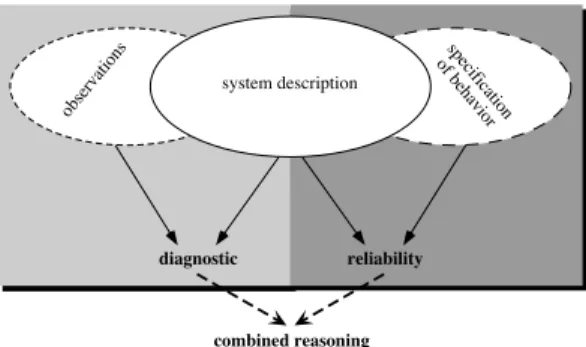
system description obs erva tions spe cifica tion of be ha vior diagnostic reliability combined reasoning
Figure 1. Reliability versus Diagnostic.
The two main problems depend both on a formalization of the system in some framework together with either observa-tions, measurements, or requirements (Fig. 1). Here, we will use the concept of probabilistic argumentation systems PAS for modeling the system description as well as observation and specifications of behaviour in one common framework. The goal of a PAS is to derive arguments in favor and against the hypothesis of interest. An argument is a defeasible proof built on uncertain assumptions, i.e. a chain of deductions based on assumptions that makes the hypothesis true. If probabilis-tic information is available, a quantitative judgement of the situation is obtained by considering the probabilities that the arguments are valid. The resulting degrees of support and pos-sibility correspond to belief and plaupos-sibility, respectively, in the Dempster-Shafer theory of evidence [24, 20]. In fact, PAS combines the strengths of logic and probability in one frame-work. In this paper we show that probabilistic argumentation systems are a framework which allows to formulate both main problems, i.e. reliability and diagnostic, easily and all concepts therefore can clearly be defined therein. The framework will especially allow to consider one common strategy for comput-ing answers to the questions in the different situations. Some work in this direction but without using PAS has been done by Provan [22].
The main information for both problems is the description of the system in some formalism; we will focus here on a
for-malization using logic. In the case of reliability, we may have a specification which describes the goals which have to be ful-filled by the system. This information will be used to compute the structure function from the system description. Different specifications may lead to different structure functions. Even in the absence of an explicit specification of a reliability re-quirement, we may deduce a structure function by assuming that the system should be functioning at least if all compo-nents are working.
On the other hand, in the case of diagnostic, some obser-vations of the system may indicate that the system is not working as it is supposed to be. This information — together with the system description — allows then to compute the di-agnoses of the system, i.e. minimal sets of components whose malfunctioning “explains” the wrong behaviour of the whole system.
2 Reliability
2.1 Combinatorial Reliability
In binary combinatorial reliability, a system is assumed to be composed of a number of different components. Each com-ponent is either intact or it is down, and so is the whole system itself, depending on the states of its components. In order to formulate this, binary variablesxiare associated to components i = 1,2, . . . , n of the system, where xi = ! if the component numberiworks andxi=⊥otherwise. Letx be the vector (x1, x2, . . . , xn) of the component states. This state-vector has 2n possible values. These values can be de-composed into two disjoint subsets, the set S" of working states, for which the system as a whole is assumed to be func-tioning, and the setS⊥of down-states, for which the system is supposed to not work properly. The corresponding system state is denoted byx. Its dependence on the state-vectorxis described by a Boolean functionφ, defined as
x = φ(x) =
!
! ifx∈S",
⊥ ifx∈S⊥. (1) The Boolean functionφis called thestructure functionof the system. In combinatorial reliability it is assumed to be given and it forms the base for reliability analysis.
The structure function φis usually assumed to be mono-tone. That is, ifx1≤x2, thenφ(x1)≤φ(x2). For a monotone structure function, a subsetP ⊆ {1,2, . . . , n}of components is called apath, ifφ(x) =!for all state-vectorsxfor which the components of the setP are working,xi=!for alli∈P. That is, the elements of a path are sufficient to guarantee the functioning of the system, regardless of the state of the com-ponents outside the path. We assume that the set{1,2, . . . , n}
of all components is a path (otherwise the system would never be functioning). A pathP is calledminimal, if no proper sub-set ofP is still a path. Since the paths are upwards closed it is sufficient to know all minimal paths. LetP denote the set of minimal paths. This set determines the structure function,
φ(x) = "
P∈P
# i∈P
xi. (2)
This logical formula expresses the fact, the system is working, if all components of at least one minimal path are working.
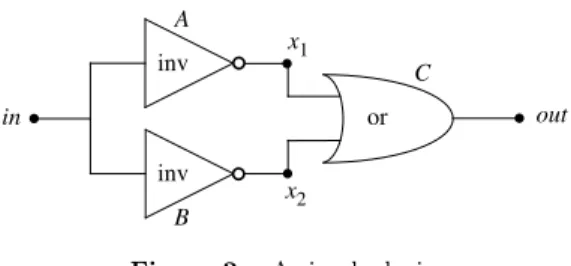
or in out inv inv A B C x1 x2
Figure 2. A simple device
Dually, the notion of acut is defined andCdenotes the set of all minimal cuts.
If for every componenti= 1,2, . . . , n its respective prob-ability pi of functioning correctly is defined, then the prob-ability that the system is functioning can be computed (as-suming the components to be stochastically independent). In fact,φ(x) is a random variable, and the probabilitypthat the system is functioning is
p=E(φ(x)) =h(p). (3)
Here, p denotes the vector (p1, p2, . . . , pn) of probabilities. h(p) is called the reliability function and its computation is a nontrivial task [1, 16, 5].
2.2 Model-Based Reliability
The structure function describes the conditions under which a system is functioning, depending on the states of its com-ponents. It is already a compilation of knowledge about the system and its structure. In this section we shall illustrate an-other approach, where a more physical description of a system is given. Additionally, a specification of the desired behavior of the system is given. These two elements will then allow the deduction of a structure function and its associated reliability function. The discussion in this section will be informal. Example 1: Detector of Power Failure
(Example adapted from [22])
Consider a simple device which watches a Boolean valuein
and reports an outputoutequal to!, if the value vanishes (becomes⊥). A simple version of such a device is depicted in Figure 2. The functionality of this device can be described with propositional logic. Letinandoutbe the variables which denote the state of the in- and output respectively. Both vari-ables are binary, i.e. represent the boolean values true or false respectively. Further, there are two internal variablesx1 and x2, also binary. For every componentA,B or C, there is a respective binary variableokA,okB, andokC which describes the working mode of the component.
Consider the inverterA: if it works correctly (okA is true), then its input is the negation of its output,outis true if and onlyinis false. We express this by the formulain↔ ¬x1. So the entire information is modeled as the logical implication
okA → (in ↔ ¬x1). Note that so far nothing is said about the behavior of the component, if it is down (okA is false). There are several possibilities. One is that in this case the output of the component is always false, i.e.¬okA→ ¬x1.
For the component B, the same specification can be ap-plied. For the or-gate, if it works correctly, then the output is
true if at least one of its inputs is. So the whole information about the device is modeled by a set of six implications:
Σ = okA→(in↔ ¬x1), ¬okA→ ¬x1, okB→(in↔ ¬x2), ¬okB→ ¬x2, okC→(out↔x1∨x2), ¬okC→ ¬out (4)
This is thesystem description. We add now a specification of what we expect from the system to this physical description of the system. We expect, that negative (false) input is detected, i.e. the output is true. This could be expressed by¬in→out. However, this is a weak requirement. It does not exclude that
outbecomes true, even ifinis true. More stringent would be the specification¬in↔out. This asks that there is an alarm (out) if, and only if,inis false.
We may now ask under which states, described by the vari-ables okA,okB, andokC, each one of these specifications is fulfilled. This defines thestructure function of the system as-sociated with the corresponding specification of desired sys-tem behavior. We shall see in the next section, that it is a well-defined problem of propositional logic to deduce these structure functions from the system description and the spec-ifications of desired behavior. )
This example shows how the physical behavior of systems and the required behavior can be described in the language of propositional logic. We shall examine this structure in the following section in a general context.
3 Probabilistic Argumentation Systems
Probabilistic argumentation systems have been developed as general formalisms for expressing uncertain and partial know-ledge and information in artificial intelligence. They combine in an original way logic and probability. Logic is used to derive arguments and probability serves to compute the reliability or likelihood of these arguments. These systems can be used for model-based diagnostics as has been demonstrated in [2, 19]. Here we shall show how they relate to reliability theory.In this section we give a short introduction into proposi-tional probabilistic argumentation systems. For a more de-tailed presentation of the subject we refer to [15]. We remark also that such systems have been implemented in a system called ABEL which is available on the internet (cf. [14] for further information).
3.1 Propositional Logic
Propositional logic deals with declarative statements, called called propositions, that can be either true or false. Let
P = {p1, . . . , pn} be a finite set of propositions. The sym-bolspi ∈P together with!(tautology) and⊥(falsity), are called atoms. Compound formulas are built by the following syntactic rules:
• atoms;
• ifγis a formula, then¬γis a formula;
• ifγ andδare formulas, then (γ∧δ), (γ∨δ), (γ→δ), and (γ↔δ) are formulas.
By assigning priority in decreasing ordering to ¬,∧, ∨, →, some parentheses can be eliminated. The setLP of all formu-las generated by the above recursive rules is called
proposi-tional language overP.
A literal is either an atompi or the negation of an atom
¬pi. A term is either ! or a conjunction of literals where every atom occurs at most once (but none of⊥and!), and
aclause is either ⊥or a disjunction of literals where every
atom occurs at most once (but none of⊥and!).CP ⊆ LP denotes the set of all terms, andDP the set of all clauses.
NP ={0,1}n denotes the set of all 2n different interpreta-tions forP. Ifγ∈ LP evaluates to 1 underx∈NP, thenxis called amodel ofγ. The set of all models ofγ is denoted by
NP(γ)⊆NP.
A propositional sentenceγentails another sentence δ (de-noted byγ |=δ) if and only ifNP(γ)⊆NP(δ). Sometimes, it is convenient to writex |= γ instead of x ∈NP(γ). Also we writeγ|=⊥ifγ is not satisfiable. Furthermore, two sen-tencesγ andδ arelogically equivalent (denoted byγ≡δ), if and only ifNP(γ) =NP(δ).
3.2 Basic Concepts of Argumentation
Systems
Consider two finite sets P = {p1, . . . , pm} and A =
{a1, . . . , an}of propositional variables withA∩P =∅, the ele-ments ofP are called propositions, the elements ofA assump-tions. We consider a fixed set of formulas Σ⊆ LA∪Pcalled the
knowledge base, which models the information available; sets
of formulas are interpreted conjunctively, i.e. Σ =*{ξ∈Σ}. We assume that this knowledge base is satisfiable. A triple (Σ, A, P) is called apropositional argumentation system PAS. The elements ofNAare calledscenarios(orsystem states). A scenario represents a specification of all values of the as-sumptions inA. Define now:
Inconsistent Scenarios: CSA(Σ) :={s∈NA:s,Σ|=⊥},
Quasi-Supporting Scenarios ofh∈ LN:
QSA(h,Σ) :={s∈NA:s,Σ|=h},
Supporting Scenarios ofh∈ LN:
SPA(h,Σ) :=QSA(h,Σ)−CSA(Σ),
Possible Scenarios forh∈ LN:
PLA(h,Σ) :=SPAc(¬h,Σ). Inconsistent scenarios are in contradiction with the know-ledge base and therefore to be considered as excluded by the knowledge. Supporting scenarios for a formulahare scenar-ios, which, together with the knowledge base imply h and are consistent with the knowledge. So, under supporting sce-narios, the hypothesishis true. Possible scenarios forhare scenarios, which do not imply¬hand thereby do not refuteh. Quasi-supporting scenarios forhare the union of supporting scenarios and inconsistent scenarios.
Scenarios are the basic concepts of assumption-based rea-soning. However, sets of inconsistent, quasi-supporting, sup-porting and possible scenarios may become very large. There-fore, more economical, logical representations of these sets are needed. For this purpose, the following concepts are defined:
Set of Supporting Argument forh:
SP(h,Σ) ={α∈CA:NA(α)⊆SPA(h,Σ)}, The sets of quasi-supporting and of possible arguments are defined analogously. Remark that supporting arguments are similar to paths for structure functions in reliability the-ory. This similarity will be exploited later. These sets are
all upward closed. Hence the sets of arguments are al-ready determined by their minimal elements. We denote by
µQS(h,Σ), µSP(h,Σ) and µPL(h,Σ) the sets of minimal quasi-supporting, supporting and possible arguments. Fur-ther, Conflict: conf(Σ) := " α∈µQS(⊥,Σ) α, Support ofh: sp(h,Σ) := " α∈µSP(h,Σ) α,
Quasi-support qs(h,Σ) and possibility pl(h,Σ) are defined analogously. Clearly, any formula which is logically equivalent to logical representations above can be used as a representa-tion.
Example 2: (Cont. of Example 1)
The information of Example 1 is modeled in an argu-mentation system as follows: A = {okA, okB, okC}, P =
{in, x1, x2, out} and Σ as in (4). There are no incon-sistent scenarios and for h = ¬in → out we have
QSA(h,Σ) = {(0,1,1),(1,0,1),(1,1,1)} and PLA(h,Σ) = NA. As CSA(Σ) =∅, we have QSA =SPA in this situation and there are some arguments in favor of the hypothesis, but none against it. Hence,qs(h,Σ) = (okA∧okC)∨(okB∧okC)
andpl(h,Σ) =!. )
3.3 Probabilistic Information
On top of the structure of a propositional argumentation sys-tems, we may easily add a probability structure. Assume that there is a probabilityp(ai) =pifor every assumptionai∈A given. Assuming stochastic independence between assump-tions, a scenarios= (s1, . . . , sn) gets the probability
p(s) = n + i=1 psi i (1−pi) 1−si. (5)
This induces a probability measureponLA,
p(f) = ,
s∈NA(f) p(s)
forf∈ LA. A quadruple (Σ, A, P,Π) with Π = (p1, . . . , pn) is then called aprobabilistic (propositional) argumentation
sys-tem PAS.
The problem of computing the probabilityp(f) is similar to the problem of computing the reliability of a structure func-tion, except, that monotonicity cannot be assumed in general; for algorithms for efficiently computing the probability p(f) see [20, 9, 13].
Once we have such a probability structure on top of a propositional argumentation system, we can exploit it to com-pute likelihoods (or in fact, reliabilities) of supporting and possible arguments for hypothese h. First, we note, that Σ imposes that we eliminate the inconsistent scenarios and con-dition the probability on the consistent ones. In other words, Σ is an event that restricts the possible scenarios to the set
NA−CSA(Σ), hence their probability has to be conditioned on the event Σ. This conditional probability is defined by
p'(s) = p(s) 1−p(qs(⊥,Σ)).
for consistent scenarioss.p(qs(h,Σ)) =dqs(h) is the so-called degree of quasi-support forh. Now, the degree of supportdsp
for hypotheseshis defined by
dsp(h) =p'(sp(h,Σ)) = dqs(h,Σ)−dqs(⊥,Σ) 1−dqs(⊥,Σ) .
This result explains the importance of quasi-support. It is sufficient to compute degrees of quasi-supports. Further, we obtain the degree of plausibility ofh,
dpl(h) =p'(pl(h,Σ)) = 1−dqs(¬h,Σ)
1−dqs(⊥,Σ) = 1−dsp(¬h). Degree of quasi-supportdqs(h) and of supportdsp(h) corre-spond in fact to unnormalized and normalized belief in the Dempster-Shafer theory of evidence [24, 20, 15].
3.4 Computational Theory
Computing quasi-supports is the basic operation in PAS. It can be based on resolution and variable elimination (forget-ting) [15, 12, 13]. In the sequel, we will sketch some of the main concepts for computation.
First, note that the computation ofqs(h) can be reduced to the computation of the conflicts with respect to an updated knowledge base: qs(h,Σ) = qs(⊥,Σ∪ {¬h}). So for any hy-pothesish, the quasi-supporting arguments qs(h,Σ) can be determined by computing the conflicts with respect to the knowledge base Σ∪ {¬h}. Hence in the sequel, we focus on the computation of the conflicts with respect to a general knowledge base.
The ideas presented in the sequel are based on representa-tions of knowledge in conjunctive normal form (CNF), i.e. a conjunction of clauses. The main step is based on the princi-ple of resolution. Letx∈A∪P. A disjoint decomposition of Σ is then defined as follows:
Σ+x = {ξ∈Σ :x∈Lit(ξ)} Σ−x = {ξ∈Σ :¬x∈Lit(ξ)}
Σ0x = {ξ∈Σ :x /∈Lit(ξ) and¬x /∈Lit(ξ)} Lit(Σ) denotes the set of all literals occurring in Σ. A literal is either a (positive) atom or a negated atom.
Consider two clausesξ+=x∨δ+andξ−=¬x∨δ−in Σ+ x and Σ−
x respectively. The clauseρ(ξ+, ξ−) =δ+∨δ−is called the resolvent; note that we simplify implicitly the resolvent so thatρ(ξ+, ξ−) is again a clause, i.e. double occurrences of atoms etc. are simplified.
Eliminating a variable x ∈ P ∪A from Σ means now to compute
Elimx(Σ) =µ(Σ0x∪ {ρ(ξ+, ξ−) :ξ+∈Σ+x, ξ−∈Σ−x}) Consider a setQ⊆P∪A. We define now, forQ={q1, . . . , qr},
ElimQ(Σ) =Elimqr(. . .(Elimq2(Elimq1(Σ))). . .)
The result does not depend on the very order of the elimina-tion of atoms; yet note that the computaelimina-tions depend criti-callyon a “good” ordering, see [15] for a discussion as well as relations to the theory of local computation (in the sense of Shenoy & Shafer [25]).
This allows then to compute the quasi-supporting argu-ments of a knowledge base Σ as follows:
Theorem 1 ([15])
QSA(h,Σ) =NAc(ElimP(Σ∪ {¬h})) In other words, this theorem asserts that
qs(h,Σ)≡ ¬#ElimP(Σ∪ {¬h}).
The concept of elimination allows to compute quasi-supporting and therefore also quasi-supporting as well as possible arguments for hypotheses. This notation connects the con-cepts presented here to the more general theory of valuation algebras, a general theory for representing, combining and fo-cusing pieces of information [18, 21].
4 Reliability Analysis Using Probabilistic
Argumentation Systems
4.1 Reliability based on Requirement
Specification
We discuss now how probabilistic argumentation systems can be used to formulate and solve reliability problem. The ba-sic idea is simple: The system behavior is described in terms of the states of its components. In addition the desired or re-quired behavior of the system is specified. The system descrip-tion forms a probabilistic argumentadescrip-tion system. The ques-tion is then: how likely (probable) is it, that the specified requirement is satisfied? In order to answer this question, the specification of required behavior is taken as a hypothesis.
Thesupport of this specification determines then essentially
the structure function of this reliability problem, and the de-gree of support of the specified requirement is the reliability of the system with respect to the required behavior. Note that — depending on different goals a system should attain, or services it should provide — different requirements may be formulated. So the corresponding reliability analysis has to be differentiated, but can be carried out within the same framework of probabilistic argumentation systems.
Example 3: (Cont. of Example 1)
We have already formulated Σ and two different specifications
δ1 =¬in →out andδ2 =¬in ↔out. We can compute the supports of these two specifications. It turns out, that both are the same,
sp(δ1,Σ) =sp(δ2,Σ) = (okA∧okC)∨(okB∧okC). Note that this is just the path representation of the expected structure function. In fact this structure function could be reformulated as (okA∨okB)∧okC, which shows that it is a series system composed of componentCand a parallel module of the componentsAandB. The remarkable fact is, that this structure function has been automatically deduced from the system description and the specification of requirements.
The system description is an essential element for this anal-ysis. If it is changed, then this may influence the results of the analysis. Suppose that, in contrast to the model above, we do not know how the faulty components behave. The knowledge base becomes now
Σ'=
!
okA→(in↔ ¬x1), okB→(in↔ ¬x2), okC→(out↔x1∨x2).
-With this less complete model, the structure function of the two specifications above become different,
sp(δ1,Σ') = (okA∧okC)∨(okB∧okC), sp(δ2,Σ') = okA∧okB∧okC.
Now, the stronger requirementδ2 can only be guaranteed if all three components work correctly (a series system), whereas the weaker one still has the same redundancy as before. )
In the general case, we have a PAS (Σ, A, P), where the assumable symbols inAcorrespond to the components of the system. Positive assumptions correspond to working compo-nents. Accordingly in the context of reliability analysis, we shall call the scenarios of this argumentation systemsystem
states. The propositional symbols inP are needed to describe
the system behavior. We assume that the system descrip-tion Σ excludes no system states, that is there are no con-flicts, QSA(⊥,Σ) = ∅. A knowledge base Σ which satisfies this is calledA-consistent.
The required behavior is specified by a formulaδ. Usuallyδ
will not contain assumptions, but there is no reason to exclude this in general.δ formulates a reliability goal. There may be several such goals.
The set of system statesSPA(δ,Σ) supportingδcontains all states guaranteeing the required specification from the sys-tem description. Its complement SPAc(δ,Σ) = PLA(¬δ,Σ) contains the system states where this guarantee is no more assured. These are the unreliable states. SoSPA(δ,Σ) defines
thestructure function associated with the specificationδ
s = φδ,Σ(s) =
!
! ifs∈SPA(δ,Σ),
⊥ ifs∈/SPA(δ,Σ). (6) The index Σ inφδ,Σwill be omitted if Σ is clear from the con-text. Here,sdenotes the “system state”, which is!, when the reliability specification is assured and⊥otherwise. Since the setSPA(δ,Σ) has a logical representation based on minimal arguments, the same holds for the structure functionφδ,
φδ= " α∈µSP(δ,Σ)
α =sp(δ,Σ) (7)
In the same way, based on minimal possible arguments
P L(¬δ,Σ), we obtain
¬φδ= " β∈µPL(¬δ,Σ)
β =pl(¬δ,Σ).
By de Morgan laws this transforms into
φδ= # β∈µPL(¬δ,Σ)
¬β. (8)
Note that¬β, the negation of a term, is a clause. This is a second logical representation ofφδ.
A comparison with the minimal path and minimal cut rep-resentation of monotone structure functions (2) shows that minimal supporting argumentsαfor δand minimal possible argumentsβfor ¬δplay a role similar to minimal paths and minimal cuts.
According to our assumption of A-consistency, we have
QSA(⊥,Σ) =∅. Thus
On the other hand, we have also
PLA(¬δ,Σ) =QSA c
(⊥,Σ∪ {¬δ}). (10) This shows, that a reliability analysis of a system Σ relative to a requirement specificationδ, requires essentially the com-putation of the conflict statesQSA(⊥,Σ∪ {¬δ}). We shall see below, that this is exactly also what is required for diagnosis. This is a first hint to the duality between the problems of reliability and diagnosis.
Once probabilities for the assumptions, i.e. component availabilities or reliabilities are defined, system reliability rel-ative to a specificationδis simply the degree of support ofδ, (sinceQSA(⊥,Σ) =∅), i.e.
pδ,Σ=dsp(δ,Σ) =dqs(δ,Σ) =p(QSA(⊥,Σ∪ {¬δ})).
4.2 Implicitly Defined Reliability
A specificationδis calledconsistent with the system descrip-tion Σ, if the system state1belongs toSPA(δ,Σ). In this sec-tion we only consider specificasec-tions consistent with the system description.
A system description Σ often contains, besides assumptions, another set O of special propositional atoms, namely those which are observable. Then specifications δ can be assumed to be formulated with observables only,δ∈ LO. Observables are typically input and output variables of some system.
Assume now, that in a system description (Σ, P, A) a set of observable variables Ois singled out. Usually, O⊆P, i.e. component states can not be observed directly. But it does no harm to assume more generally O⊆P ∪A. Then we define an implicit specification
ˆ
δ=Elim(A∪P)−O(Σ∪ {a1∧a2∧ · · · ∧an}).
That is, ˆδ represents all the functionality of the system in terms of observables which can be obtained from a system with all components working. We call this theimplicit relia-bility specification with respect toO. Now, the system may be — with respect to this specification — as good as “new” also for some states including faulty components. Therefore we define the implicit structure function by the set of up-states relative to ˆδ, i.e.SPA(ˆδ,Σ). Hence, we obtain
φˆδ= " α∈µSP(ˆδ,Σ) α, or φδˆ= # β∈µPL(¬δ,Σ)ˆ ¬β.
Accordingly, the implicit reliability of such a system can be obtained as the degree of support dsp(ˆδ,Σ). This approach helps to decide whether a system has some implicit redun-dancy, namely, whetherφˆδrepresents simply a series system, i.e.µSP(ˆδ,Σ) has only the set of all assumptions as minimal supporting argument for ˆδ.
Lemma 2 Ifδ∈ LO is a consistent specification with respect toΣ, thenˆδ|=δ.1
This shows that ˆδ is the most stringent, consistent speci-fication over observablesO. For all specifications overOthe implicit specification has least reliability:
1 For proofs see [6].
Lemma 3 Ifδ∈ LOis a consistent specification with respect toΣ, then SPA(ˆδ,Σ)⊆SPA(δ,Σ).
Corollary 4 Ifδ∈ LO is a consistent specification with re-spect toΣ, thenpˆδ≤pδ.
5 Model-Based Diagnostic
5.1 Duality Between Reliability and
Diagnostics
A problem of diagnostics arises if an observation indicates that a requirement specificationδis violated. Then the ques-tion is: how can the required funcques-tionality be recovered? That is, one would like to find out those components whose fail-ure caused the system failfail-ure and which have to be fixed or replaced. This analysis will be based on the system descrip-tion Σ and on the specificadescrip-tionδwhich is violated.
In fact, we ask, which system states are compatible or con-sistent with the system description Σ and the violation of the specificationδ, expressed by¬δ. Well, these are of course all states which are consistent with Σ∪ {¬δ}, that is the set
QSA c
(⊥,Σ∪ {¬δ}) =PLA(¬δ,Σ). (11) Remark that this is exactly the set of down states relative to the specificationδ (see (10)). Here we have the basicduality
between reliability analysis relative to a requirement speci-fication δ and the diagnostic problem relative to the same specification. The conflict setQSA(⊥,Σ∪ {¬δ}) is the com-putational key to both reliability analysis and diagnostics. It gives the up-states which define reliability and its complement gives the possible states explaining the violation of the relia-bility specification, i.e. possible diagnostics. It is well known in model-based diagnostics that such conflict sets play a key role [23, 10, 19]. The duality implies that they play an equally important role for model-based reliability.
If the structure functionφδ,Σismonotone, then to the min-imal possible argumentsβ∈µPL(¬δ,Σ) correspond the min-imal cuts¬β. They represent minimal sets of failed compo-nents, which explain the violation of the specificationδ, inde-pendently on the state of the other components.
Minimal cuts correspond to kernel diagnoses in model-based diagnostics [23]. Usually model-model-based diagnostics goes not beyond such concepts of diagnostics. It neglects the im-portant role of probability.2 The observation of the violation of the specification¬δ in fact defines the eventQSAc(⊥,Σ∪
{¬δ}) in the sample spaceNA. That is, the prior probabilities p(s) defined on the states have now to be conditioned on this event. This gives us theposterior probabilities
p(s|¬δ) = p(s)
1−p(QSA(⊥,Σ∪ {¬δ}))
= p(s)
dpl(¬δ,Σ), (12) for diagnostic statess∈ QSA(⊥,Σ∪ {¬δ}). This underlines once more the key role of the conflict setQSA(⊥,Σ∪{¬δ}). Its prior probability is sufficient to compute the posterior proba-bilities of the possible diagnostic states explaining the viola-tion ofδ.
2 See however [19, 3] for a discussion of this subject, and
es-pecially [19] for the problems of the approach of De Kleer & Williams [11]. Other approches focus for example on minimal entropy [26] or on restricting the device to have a Bayesian net-work model [17].
These posterior probabilities represent important adtional diagnostic information. For example we may look for di-agnostic states with maximal posterior probability. ˜sis called amaximal likelihood state, if
p(˜s|¬δ) = max
s∈QSAc(⊥,Σ∪{¬δ})p(s|¬δ). (13) There may be several such states. They represent most likely states explaining the violation ofδ.
Reiter [23] proposed to look especially at possible diagnos-tic states with a minimal number of faulty components. In-tuitively this makes sense: The failure should be explained with a minimal number of down components. Ifsis a state, we define s− to be the set of its negative (down) compo-nents. Then we define a partial order between states: s' ≤s ifs'−⊆s−.Reiter diagnosesare now those diagnostic states
s ∈ QSAc(⊥,Σ∪ {¬δ}), which are minimal with respect to this partial order. We make the reasonable assumption that for every componentiwe havepi>0.5 such thatpi>1−pi. I.e. it is more probable that a component works than that it is down. Then s' <s implies that p(s'|¬δ) > p(s|¬δ). So maximum likelihood states are Reiter diagnoses. The inverse of course does not hold necessarily. Also, if the structure func-tionφδis monotone, thes−of Reiter diagnoses correspond to minimal cuts relative to the specificationδ.
The posterior fault probabilities of the components,
p(¬ai|¬δ), are also of interest. The larger this probability, the more critical is componentifor the requirement specifi-cation δ. So this is a possible importance measure for com-ponent i relative to the specification (for other importance measures see [4]).
Example 4: (Cont. of Example 1)
Suppose we observe that, although ¬in, we have also ¬out, i.e. a power system failure is not detected. Note that¬in∧ ¬out≡ ¬δ1 (cf. Example 3). So we consult the minimal cuts relative to the specification¬δ1. There are two minimal cuts:
{¬okC}and{¬okA,¬okB}. To any minimal cut corresponds a Reiter diagnosis, namely,{okA, okB,¬okC}to the first cut, and {¬okA,¬okB, okC}to the second one. One of these two diagnoses must be the maximum likelihood state. The first one has prior probability 0.99×0.99×0.05 = 0.049, the second one 0.01×0.01×0.95 = 0.000095. So clearly, the first one is by far the most likely state. The posterior probability is obtained by dividing the prior probability by the unreliability 0.05 relative toδ1. We obtain for the maximum likelihood state a posterior
probability of 0.98. )
5.2 Diagnostics Based on Observations of
System Behavior
The actual observation is not necessarily the negation of a sys-tem requirement, but may be something stronger, which im-plies the violation of a specification. Indeed, as we saw in Ex-ample 4 we observed¬in∧¬out≡ ¬δ1, but¬in∧¬out|=¬δ2. So, we should reconsider the duality between reliability and diagnostics. In fact, assume that we make some observation of the system behavior, expressed in a formulaωover observ-ables. Then we may test whetherω|=¬δˆΣ. If this is the case, then we have a diagnostic problem, in the sense that at least one component must be down.
The solution of this diagnostic problem is found along sim-ilar lines as in the previous section. Possible states are those, which are consistent with the system description and the ob-servation. Or, in other words, the states in the conflict set
QSA(⊥,Σ∪ {ω}) are those which are excluded by the obser-vation. So, the possible diagnostic states are those of the set
PLA(ω,Σ) =QSAc(⊥,Σ∪ {ω}). We see that this diagnostic problem is dual to a (fictitious) reliability problem with a “re-quirement” specification¬ω. Note that the specification¬ωis always consistent with Σ, since ˆδΣis consistent andω|=¬ˆδΣ. Of course, we get a much sharper diagnostic with an ob-servationω|=¬δˆ, than with the information of¬ˆδonly. This follows, because according to Lemma 3, we havePLA(ω,Σ)⊆ PLA(ˆδ,Σ). So, the more precise the observation, the more states are eliminated. A mere statement that a given reliabil-ity specification is violated is less informative than a precise observation implying a violation of a requirement specifica-tion.
6 Combining Diagnostic and Reliability
We conclude this discussion of duality between reliability and diagnostics by remarking that we may have an observation of the system behavior which does neither entail a specificationδnor its violation¬δ. But still this observation is information and we can use it to improve reliability analysis and also to perform a preventive diagnostic analysis (see [6]). For relia-bility as well as for diagnostic, additional measurements — or more generally any additional information — can be taken into account in the framework presented above and helps to focus the reasoning.
7 Conclusions
In this paper we have shown how closely reliability and model-based diagnostic are connected. The framework of probabilis-tic argumentation system appears to be a framework which covers both approaches. Therefore the generic structure of PAS can be used for solving problems in both domains. The approaches can even be combined and the information spec-ified can be used in the common framework. Further, from the system description of an argumentation system, we can derive the appropriate structure function and — if desirable — take into consideration a reliability requirement. PAS al-lows to use local computation architectures and approxima-tion techniques [25, 15]. This complements the computaapproxima-tional theory of reliability theory.
REFERENCES
[1] J. A. Abraham, ‘An improved algorithm for network reliabil-ity’,IEEE Transactions on Reliability,28, 58–61, (1979). [2] B. Anrig, ‘Probabilistic argumentation systems and
model-based diagnostics’, in DX’00, Eleventh Intl. Workshop on Principles of Diagnosis, Morelia, Mexico, eds., A. Darwiche and G. M. Provan, pp. 1–8, (2000).
[3] B. Anrig,Probabilistic Model-Based Diagnostics, Ph.D. dis-sertation, University of Fribourg, Institute of Informatics, 2000.
[4] B. Anrig, ‘Importance measures from reliability theory for probabilistic assumption-based reasoning’, inEuropean Conf. ECSQARU’01, Toulouse, eds., S. Benferhat and P. Besnard, pp. 692–703. Lecture Notes in Artif. Intell., Springer, (2001).
[5] B. Anrig and F. Beichelt, ‘Disjoint sum forms in reliability theory’,ORiON J. OR Society South Africa,16(1), 75–86, (2001).
[6] B. Anrig and J. Kohlas, ‘Model-based reliability and diag-nostic: A common framework for reliability and diagnostics’, Technical Report 02-01, Department of Informatics, Univer-sity of Fribourg, (2002).
[7] R. E. Barlow and R. Proschan,Statistical Theory of Reliabil-ity and Life Testing, New York, 1975. IAUTOM 3.9.4-10. [8] F. Beichelt, Zuverl¨assigkeits- und Instandhaltungstheorie,
Teubner, Stuttgart, 1993.
[9] R. Bertschy and P.-A. Monney, ‘A generalization of the algo-rithm of Heidtmann to non-monotone formulas’,J. of Com-putational and Applied Mathematics,76, 55–76, (1996). [10] R. Davis, ‘Diagnostic reasoning based on structure and
be-haviour’,Artif. Intell.,24, 347–410, (1984).
[11] J. De Kleer and B. C. Williams, ‘Diagnosing multiple faults’,
Artif. Intell.,32, 97–130, (1987).
[12] R. Haenni, ‘Cost-bounded argumentation’,Int. J. of Approx-imate Reasoning,26(2), 101–127, (2001).
[13] R. Haenni, ‘A query-driven anytime algorithm for assumption-based reasoning’, Technical Report 01-26, University of Fribourg, Department of Informatics, (2001). [14] R. Haenni, B. Anrig, R. Bissig, and N. Lehmann. ABEL
homepage. http://diuf.unifr.ch/tcs/abel, 2000.
[15] R. Haenni, J. Kohlas, and N. Lehmann, ‘Probabilistic ar-gumentation systems’, inHandbook of Defeasible Reasoning and Uncertainty Management Systems, eds., J. Kohlas and S. Moral, volume 5: Algorithms for Uncertainty and Defeasi-ble Reasoning, Kluwer, Dordrecht, (2000).
[16] K. D. Heidtmann, ‘Smaller sums of disjoint products by sub-product inversion’,IEEE Transactions on Reliability,38(3), 305–311, (August 1989).
[17] P. H. Ibarg¨uengoytia, L. E. Sucar, and E. Morales, ‘A probabilistic model approach for fault diagnosis’, inDX’00, Eleventh Intl. Workshop on Principles of Diagnosis, More-lia, Mexico, eds., A. Darwiche and G. M. Provan, pp. 79–86, (2000).
[18] J. Kohlas. Valuation algebras: Generic architecture for rea-soning. draft, 2002.
[19] J. Kohlas, B. Anrig, R. Haenni, and P.-A. Monney, ‘Model-based diagnostics and probabilistic assumption-‘Model-based reason-ing’,Artif. Intell.,104, 71–106, (1998).
[20] J. Kohlas and P.-A. Monney, A Mathematical Theory of Hints. An Approach to the Dempster-Shafer Theory of Evi-dence, volume 425 ofLecture Notes in Economics and Math-ematical Systems, Springer, 1995.
[21] J. Kohlas and R. F. St¨ark, ‘Information algebras and informa-tion systems’, Technical Report 96–14, University of Fribourg, Institute of Informatics, (1996).
[22] G. M. Provan, ‘An integration of model-based diagnosis and reliability theory’, in DX’00, Eleventh Intl. Workshop on Principles of Diagnosis, Morelia, Mexico, eds., A. Darwiche and G. M. Provan, pp. 193–200, (2000).
[23] R. Reiter, ‘A theory of diagnosis from first principles’,Artif. Intell.,32, 57–95, (1987).
[24] G. Shafer,The Mathematical Theory of Evidence, Princeton University Press, 1976.
[25] P. P. Shenoy and G. Shafer, ‘Axioms for probability and belief functions propagation’, inUncertainty in Artif. Intell. 4, eds., R. D. Shachter, T. S. Levitt, L. N. Kanal, and J. F. Lemmer. North Holland, (1990).
[26] P. Struss, ‘Testing for discrimination of diagnoses’, inDX’94, Fifth Intl. Workshop on Principles of Diagnosis, New Paltz, USA, (1994).