MSSD DISCUSSION PAPER NO. 49
Markets and Structural Studies Division
International Food Policy Research Institute
2033 K Street, N.W.
Washington, D.C. 20006 U.S.A.
http://www. ifpri.org
November 2002
MSSD Discussion Papers contain preliminary material and research results, and are circulated prior to a full peer review in order to stimulate discussion and critical comment. It is expected that most Discussion Papers will eventually be published in some other form, and that their content may also be revised. This paper is available at http://www.cgiar.org/ifpri/divs/mssd/dp.htm
POVERTY MAPPING WITH AGGREGATE CENSUS DATA:
WHAT IS THE LOSS IN PRECISION?
ACKNOWLEDGMENTS
We thank Phan Xuan Cam and Nguyen Van Minh for their help understanding the Vietnam Census data and Peter Lanjouw for helpful methodological discussions. We also benefited from useful comments from participants at the conference “Understanding poverty and growth in sub-Saharan Africa” at the Centre for the Study of African
Economies, St. Catherine’s College, Oxford University, 18-19 March 2002. The usual disclaimers apply.
i
ABSTRACT
Spatially disaggregated maps of the incidence of poverty can be constructed by combining household survey data and census data. In some cases, however, statistical authorities are reluctant, for reasons of confidentiality, to release household-level census data. This paper examines the loss in precision associated with using aggregated census data, such as village- or district-level means of the data. We show analytically that using aggregated census data will result in poverty rates that are biased downward (upward) if the rate is below (above) 50 percent and that the bias approaches zero as the poverty rate approaches zero, 50 percent, and 100 percent. Using data from Vietnam, we find that the average absolute error in estimating provincial poverty rates is about 2 percentage points if the data are aggregated to the enumeration-area level and around 3-4 percentage points if they are aggregated to the provincial level. Even census data aggregated to the
provincial level perform reasonably well in ranking the 61 provinces by the incidence of poverty: the average absolute error in ranking is 0.92.
ii
TABLE OF CONTENTS
1. Introduction ... 1
2. Data and Methods... 4
Data... 4
Methods ... 5
3. Results ... 10
Provincial Estimates of Poverty In Vietnam ... 10
Determinants of the Errors of Aggregation ... 14
Empirical Comparison of Alternative Methods... 16
4. Summary and Discussion ... 24
References... 27
iii
LIST OF TABLES
Table 1—Summary of alternative methods to be compared ... 9
Table 2—Semi-log regression model of per capita expenditure ... 11
Table 3—Probit regression model of poverty... 12
Table 4—Regional and national poverty estimates using different methods ... 17
Table 5—Errors in regional poverty estimated using different methods... 19
iv
LIST OF FIGURES
Figure 1—Incidence of poverty by province ... 13 Figure 2—Comparison of provincial poverty estimates using household level census data
and using enumeration area means... 22 Figure 3—Comparison of provincial poverty estimates using household level census data
POVERTY MAPPING WITH AGGREGATE CENSUS DATA: WHAT IS THE LOSS IN PRECISION?
Nicholas Minot1 and Bob Baulch2
1. INTRODUCTION
Policymakers and researchers are interested in the geographic distribution of poverty for several reasons. First, knowledge of these patterns facilitates the targeting of programs designed, at least in part, to reduce poverty. Many countries use some form of geographic targeting in government programs such as credit, food aid, input distribution, health care, and education. Second, this information is useful in monitoring progress in addressing poverty and regional disparities. Third, it may provide some insight regarding the geographic factors associated with poverty, such as access to markets, climate, or topography.
In a growing number of countries, high-resolution poverty maps are now being produced using a relatively new two-step approach. In the first step, household survey data are used to estimate econometrically the relationship between poverty (or household expenditure) and a series of household characteristics, including household size and composition, education, occupation, housing characteristics, access to utilities, and ownership of consumer goods such as radios and bicycles. In the second step, this
1 Research Fellow, Markets and Structural Studies Division, International Food Policy Research Institute.
Washington, D.C. Email: [email protected]
2
relationship is applied to census data on the same household characteristics to calculate an estimate of the incidence of poverty for some small geographic unit. In some cases, other poverty measures and indicators of income inequality can also be calculated.
In an early application of this approach, Minot (1998, 2000) combined a probit regression on data from the 1993 Vietnam Living Standards Survey and district-level means of the household characteristics from the 1994 Agricultural Census to estimate the ranking of the incidence of poverty across 543 rural districts. Hentschel et al (1998, 2000) use household survey data and household-level census data to estimate
disaggregated poverty rates for Ecuador. They show that with household-level census data it is possible to generate unbiased estimates of the poverty rate as well as estimates of the standard error of the poverty rates. In the first stage of this approach, the logarithm of per capita expenditure is regressed on household characteristics from a household survey. In the second stage, data on the same household characteristics from the Census is used to predict per capita expenditures and derive various poverty (and inequality) measures. Poverty maps that combine household survey and census data have been prepared for Guatemala, Nicaragua, Panama, Peru, South Africa, Mozambique, Malawi, Cambodia, and Vietnam (see Henninger and Snel, 2002).
Researchers, however, do not always have access to household-level census data. The national statistics agencies in many (developing and industrialised) countries are reluctant to release household-level census data to researchers and international
organizations, in part because of the issue of the confidentiality of the data. For example, China and India have each conducted a census within the past two years, but only
3
district/county level results are available to outside researchers. In addition, the computational burden of processing census data, which may contain tens or even hundreds of millions of records, can be a challenge for even the most powerful desktop computers. When data access or computational burdens are constraining factors, one alternative is to use census data that has been aggregated to a higher level (such as the commune, district or province). This approach has been used in Vietnam and Gaza and the West Bank. In other words, the researcher uses a database consisting of the (for example) district-level means of all the household characteristics. An important question, therefore, is: how much precision is lost in generating poverty maps from aggregate census data? If the errors are small, then reliable poverty maps can be produced for a wider range of countries. If the errors are large, then the use of aggregated data is not advisable and researchers should focus on getting access to household-level data.
This study uses recent household survey and census data from Vietnam to assess the loss in accuracy associated with using aggregated census data instead of the original household-level census data. The results of this analysis suggest that errors from using aggregated census data in the second stage of poverty mapping are, in the case of Vietnam, about 2 percentage points on average, if the level of aggregation is low. Furthermore, the paper shows analytically and empirically that the error is close to zero when the incidence of poverty is close to zero, close to 50 percent, or close to 100 percent. Results from using aggregated census data must be interpreted with caution, however, because this approach tends to underestimate poverty rates that are below 50
4
percent and overestimate poverty rates above 50 percent, thus exaggerating differences between poor and less poor regions. 3
The paper is divided into four sections. Section 2 describes the data and methods used to compare alternative measures of the incidence of poverty using household survey data and census data from Vietnam. Section 3 presents three types of results. First, we present an updated provincial map of poverty in Vietnam based on the best available data and methods. Then, we derive analytical results regarding the factors that affect the size and direction of errors from the use of aggregate data. Finally, we generate poverty estimates using census data that has been aggregated at different levels and compare the results to those obtained from the household-level census data. Section 4 summarizes the results and draws some implications for future research in poverty mapping.
2. DATA AND METHODS
DATA
In this study, we use the 1998 Vietnam Living Standards Survey (VLSS) and the 1999 Population and Housing Census. The VLSS was carried out by the General Statistics Office (GSO) of Vietnam with funding from the Swedish International
Development Agency and the United Nations Development Program and with technical assistance from the World Bank. It surveyed a stratified random sample of 6000
households, comprising 4270 households and 1730 urban households. The VLSS sample
3In this paper, we use “poverty rate,” denoted by P
0, to refer to the percentage of households whose per
5
was based on ten strata: the rural areas of the seven regions and three urban strata (Hanoi and Ho Chi Minh City, other cities, and towns). For this analysis, we merge “other cities” and “towns” because the census data do not distinguish between these two strata.
The 1999 Census was carried out by the GSO and refers to the situation as of April 1, 1999. It was conducted with the financial and technical support of the United Nations Population Fund and the United Nations Development Program. Unit record data from the full Census are not available, but a 3 percent sample has been released on CD-ROM and forms the basis of this study. The 3 percent sample was selected by GSO using a stratified random sample of 5287 enumeration units, containing 534,139 households.
The two surveys have a number of household variables in common: household size and composition, education of the head and spouse, housing characteristics, source of water, type of sanitation facility, ownership of three consumer goods (radios,
televisions, and bicycles), and location of residence. METHODS
We begin with a description of the method of poverty mapping when household-level census data are available. As mentioned above, the first step in implementing this approach is to use household survey data to estimate per capita expenditure as a function of a variety of household characteristics.4
4Note that some ‘household’ characteristics (e.g., education or occupation of the household head) are
based on the characteristics of individual members of the household. Some studies (for example, Bigman
6 This typically takes the following semi-log form:
e X
y)= β+
ln( (1)
where y is per capita expenditure, X is a vector of household characteristics from the household survey, B is a vector of estimated coefficients, and e is the error term5.
The second step is to apply this equation to census data on the same household characteristics. If we are using household-level census data, this generates estimates of per capita expenditure for each household in the census. Hentschel et al. (1998) show that the incidence of poverty for a group of households is estimated by taking the average value of the probability that each household is poor. Taking the percentage of households whose estimated per capita expenditure is below the poverty line, while intuitively plausible, gives a biased estimate of the poverty rate. The probability that a household i is poor (P) is given by:
− Φ = σ β µ C i i X P (2)
where Φ() is the cumulative normal function, XiC is a vector of the same household
characteristics taken from the census, ß is a vector of the coefficients estimated in the first stage, µ is the poverty line, and σ is the standard error of the regression from the first stage. If region r contains N households labeled i= 1..N, the expected value of the
5 Elbers et al. (2001) discuss a number of econometric issues related to this step, including the problems of
heteroskedasticity and spatial autocorrelation. In this analysis, we do not apply adjustments for heteroskedasticity and spatial autocorrelation. To the extent that these are problems in our data, our estimated coefficients will be still be unbiased but they will be inefficient in that they do not make use of all the information available.
7 poverty rate for the region, Pr, is simply the average of the probabilities that the
individual households are poor6:
∑
∑
− Φ = = i C i i i r X N P N P σ β µ 1 1 (3) In some cases, however, the statistics bureau of the government is not willing torelease household-level census data but is willing to release aggregated data, such as the mean values of household characteristics for each district or village. The mean values of the household characteristics in the census data are then inserted into the regression equation estimated with the household survey. If it is a semi-log regression model, then equation (3) can be applied, with Xic being replaced by the census means. If a probit
equation is used to estimate poverty, then the regression equation directly generates the estimated incidence of poverty.
As noted in Minot (2000), this is not an unbiased estimate of poverty because the probit equation is non-linear. Using aggregate data ignores the variation in the household characteristics within each aggregation unit. For this reason, Minot (2000) used the results to rank districts by the incidence of poverty rather than reporting the estimated poverty rates. Even if we adopted the semi-log functional form in the first stage, the non-linearity of the cumulative normal function in equation (3) would make it impossible to get an unbiased poverty estimate using aggregated census data.
6 To simplify the presentation, we give the expression for the estimated percentage of households below the
poverty line. For the percentage of individuals below the poverty line, the expression must be modify to
8 On the issue of functional form, probit models are less sensitive to outliers in the data and less affected the relationship between expenditure and household characteristics in the higher income groups, which is less relevant for estimating poverty. On the other hand, using a probit on data that was originally continuous (like expenditure) involves discarding a lot of useful information. Furthermore, it has not been demonstrated that the probit model generates unbiased poverty estimates even when the data are not
aggregated.
In section 3.1, we present the semi-log and probit regression models to “predict” expenditure and poverty, respectively, based on household characteristics. Then we use the semi-log model and household-level census data to generate provincial estimates of the incidence of poverty in Vietnam. In section 3.2, we use a second-order Taylor series expansion to provide an analytical expression for the error associated with using
aggregate census data instead of household-level census data. This provides some information on the factors that influence the sign and magnitude of the error.
In section 3.3, we use data from Vietnam to examine the sensitivity of the results to the choice of functional form in the first stage of the procedure and to the use of aggregate census data in the second stage. Table 1 provides a summary of the methods being compared in this paper. With regard to the functional form, we compare the results obtained from using a) a probit model where the dependent variable indicates indicating whether or not the household is poor (as used by Minot (2000)) and b) the semi-log model in which the dependent variable is the logarithm of per capita expenditure (as used by Hentschel et al (2000) and other studies). With regard to the level of aggregation of
9 the census data, we compare the estimates of the incidence of poverty (often denoted by P0) from the original household-level census data (considered the most accurate estimate)
with estimates obtained from census data aggregated to the level of a) the enumeration area, b) the province, and c) the region. The poverty estimates are calculated at three levels (provincial, regional, and national). Of course, the poverty estimates cannot be more disaggregated that the census data on which they are based.
Table 1—Summary of alternative methods to be compared
Level of aggregation of poverty estimates
Province Region National
Household Semi-log model Probit model Semi-log model Probit model Semi-log model Probit model
EA Semi-log model Probit model Semi-log model Probit model Semi-log model Probit model
Province Semi-log model Probit model Semi-log model Probit model Semi-log model Probit model
Level of aggregation of the census data
Region Semi-log model Probit model Semi-log model Probit model
10
3. RESULTS
PROVINCIAL ESTIMATES OF POVERTY IN VIETNAM
As described above, the first step in the poverty mapping procedure is to use household expenditure data to estimate per capita expenditure (or poverty) as a function of household characteristics. Table 2 provides the semi-log models of per capita
expenditure in rural and urban areas using the Vietnam Living Standards Survey. Table 3 presents the rural and urban probit models of whether or not a household is poor based on the same household characteristics. The second step is to apply the regression model to census data on the same household characteristics.
If we apply the semi-log model to the household-level census data, the provincial estimates of the incidence of poverty rates can be mapped as shown in Figure 1. The map indicates that poverty, defined as the proportion of households whose per capita
expenditure is below the poverty line, is greatest in the north, bordering on China to the north and Laos to the west. These areas are mountainous and have low population densities, poor transport infrastructure, and a high proportion of ethnic minorities. Seven of these provinces have poverty rates of over 60 percent. Many of the provinces in the North Central Coast and the Central Highlands also have relatively high poverty rates, ranging from 45 percent to 60 percent. The Mekong Delta (the 12 southern-most provinces) and the Red River Delta (the cluster of small provinces in the north) have poverty rates of 25 to 45 percent.
11
Table 2—Semi-log regression model of per capita expenditure
Rural model Urban model N 4269 1730 R-squared 0.536 0.550 Variable Coefficient t Coefficient t Size of hhsize -0.0772 -19.5*** -0.0785 -8.1*** Proportion of members over 65 yrs -0.0831 -2.4** -0.1026 -1.6 Proportion of members under 15
yrs -0.3353 -9.4*** -0.2368 -3.6*** Proportion of female members -0.1177 -3.5*** 0.0386 0.5
Ethnic minority -0.0765 -1.9* 0.0142 0.2 Head completed primary education 0.0585 3.4*** 0.0616 1.7 Head completed lower secondary 0.0883 4.5*** 0.0338 1.3 Head completed upper secondary 0.0884 3.3*** 0.1368 3.2*** Head completed adv tech degree 0.1355 4.2*** 0.1603 3.5*** Head has post-secondary education 0.2552 4.9*** 0.1843 3.7*** No spouse 0.0173 1.0 0.0344 0.8
Spouse completed primary
education 0.0049 0.3 0.0642 1.9* Spouse completed lower secondary 0.0132 0.6 0.0987 2.6** Spouse completed upper secondary 0.0107 0.3 0.1912 2.7** Spouse completed adv tech degree 0.0921 2.3** 0.1285 3.2*** Spouse has post-secondary
education 0.1571 2.7*** 0.1752 3.1*** Head is leader/manager 0.1414 3.5*** 0.2312 3.0***
Head is professional/technician 0.1350 3.3*** 0.0576 1.2 Head is clerk/service worker 0.1362 3.4*** 0.0357 0.9
Head works in ag, forestry, or
fisheries -0.0163 -0.6 -0.0093 -0.2 Head is skilled worker 0.0701 1.9* 0.0071 0.2
Head is unskilled worker -0.0586 -1.7* -0.1599 -2.9*** Permanent house -0.9228 -4.3*** -0.5194 -3.4***
Semi-permanent house -0.3120 -3.6*** -0.4001 -3.8*** Permanent house x Area of house 0.2958 5.7*** 0.2001 5.4*** Semi-permanent house x Area of
house 0.1180 5.2*** 0.1403 4.6*** Has electricity 0.0765 2.7*** -0.0026 0.0
Has tap water 0.0828 1.4 0.2289 5.3*** Has other safe source of water 0.1157 4.4*** 0.0340 0.6 Has flush toilet 0.2700 5.5*** 0.1311 2.2**
Has latrine 0.0556 2.6** 0.0049 0.1 Owns television 0.2124 15.1*** 0.2167 5.5*** Owns radio 0.1009 7.0*** 0.1599 6.2*** Red River Delta 0.0314 0.6 0.0693 0.7 North Central Coast 0.0485 0.8 0.0445 0.6 South Central Coast 0.1373 2.2** 0.1460 1.9* Central Highlands 0.1708 2.1** omitted (no urban in region 5)
Southeast 0.5424 9.4*** 0.4151 5.5*** Mekong Delta 0.3011 5.1*** 0.1895 2.1**
Constant 7.5327 108.7*** 7.7538 64.7*** Source: Regression analysis of 1998 Viet Nam Living Standards Survey.
12
Table 3—Probit regression model of poverty
Rural model Urban model N=4269 N=1730 Variable Coefficient t Coefficient t Size of hhsize -0.0772 -19.5*** -0.0785 -8.1*** Proportion of members over 65 yrs -0.0831 -2.4** -0.1026 -1.6 Proportion of members under 15 yrs -0.3353 -9.4*** -0.2368 -3.6*** Proportion of female members -0.1177 -3.5*** 0.0386 0.5 Ethnic minority -0.0765 -1.9* 0.0142 0.2 Head completed primary education 0.0585 3.4*** 0.0616 1.7 Head completed lower secondary 0.0883 4.5*** 0.0338 1.3 Head completed upper secondary 0.0884 3.3*** 0.1368 3.2*** Head completed adv tech degree 0.1355 4.2*** 0.1603 3.5*** Head has post-secondary education 0.2552 4.9*** 0.1843 3.7*** No spouse 0.0173 1.0 0.0344 0.8
Spouse completed primary education 0.0049 0.3 0.0642 1.9* Spouse completed lower secondary 0.0132 0.6 0.0987 2.6**
Spouse completed upper secondary 0.0107 0.3 0.1912 2.7** Spouse completed adv tech degree 0.0921 2.3** 0.1285 3.2***
Spouse has post-secondary education 0.1571 2.7*** 0.1752 3.1*** Head is leader/manager 0.1414 3.5*** 0.2312 3.0***
Head is professional/technician 0.1350 3.3*** 0.0576 1.2 Head is clerk/service worker 0.1362 3.4*** 0.0357 0.9
Head works in ag, forestry, or
fisheries -0.0163 -0.6 -0.0093 -0.2 Head is skilled worker 0.0701 1.9* 0.0071 0.2
Head is unskilled worker -0.0586 -1.7* -0.1599 -2.9*** Permanent house -0.9228 -4.3*** -0.5194 -3.4***
Semi-permanent house -0.3120 -3.6*** -0.4001 -3.8*** Permanent house x Area of house 0.2958 5.7*** 0.2001 5.4*** Semi-permanent house x Area of
house 0.1180 5.2*** 0.1403 4.6*** Has electricity 0.0765 2.7*** -0.0026 0.0 Has tap water 0.0828 1.4 0.2289 5.3***
Has other safe source of water 0.1157 4.4*** 0.0340 0.6 Has flush toilet 0.2700 5.5*** 0.1311 2.2**
Has latrine 0.0556 2.6** 0.0049 0.1 Owns television 0.2124 15.1*** 0.2167 5.5*** Owns radio 0.1009 7.0*** 0.1599 6.2*** Red River Delta 0.0314 0.6 0.0693 0.7 North Central Coast 0.0485 0.8 0.0445 0.6 South Central Coast 0.1373 2.2** 0.1460 1.9* Central Highlands 0.1708 2.1** omitted (no urban in region 5)
Southeast 0.5424 9.4*** 0.4151 5.5*** Mekong Delta 0.3011 5.1*** 0.1895 2.1**
Constant 7.5327 108.7*** 7.7538 64.7*** Source: Regression analysis of 1998 Viet Nam Living Standards Survey.
13
14 These areas are favored by intensive irrigation of rice, fruits, and vegetables, good transportation networks, and proximity to the largest cities, Ho Chi Minh City and Hanoi. The areas with the lowest poverty rates (below 25 percent) include the province of Hanoi in the north, Da Nang on the central coast, and the Southeast region. The Southeast region includes Ho Chi Minh City, the largest and most commercially-oriented city in Vietnam. The rural areas around Ho Chi Minh City have become an important center for commercial agriculture and agro-industry. These patterns conform closely to the results from earlier studies (see World Bank, 1995; Poverty Working Group, 1999; and Minot, 2000).
DETERMINANTS OF THE ERRORS OF AGGREGATION
Suppose that we can only obtain district-level means of the household characteristics from the census and we wish to calculate district-level poverty rates. The sign and magnitude of the error associated with using aggregate census data instead of household-level census data can be estimated using a second-order Taylor expansion as follows (the derivation can be found in Appendix A):
− Φ − + − Φ ≅ − Φ
∑
µ σ β µ σ β µ σ iCβ µ σ Cβ C i C i X X X X N 2var '' 1 1 (4)where the index i refers to households, N is the number of households in the district, and C
X is the vector of district-level means of the household characteristics. The left-hand side of this equation represents the incidence of poverty as estimated from household-level census data (XiC), as described in Section 2.2. The first term on the right-hand side
15 is the (less accurate) estimate of the incidence of poverty rate obtained from the
aggregated census data (XC). The second term on the right side is the approximate error associated with using aggregate census data rather than household-level census data. 7 This error is a function of the variance in the estimated per capita expenditure within the aggregation region and the curvature of the cumulative normal function at the means of the aggregation region. 8
This equation has three implications for the error associated with using aggregate census data in poverty mapping. First, since the variance is always positive and since the second derivative of the cumulative normal function is positive (negative) when the dependent variable is below (above) 0.5, poverty estimates based on aggregated data will underestimate poverty in regions with poverty rates below 50 percent and overestimate poverty in regions with poverty rates above 50 percent. In other words, if a country has regions with poverty rates below 50 percent and others with rates above 50 percent, using aggregate data to produce a poverty map will exaggerate the differences in poverty between the two sets of regions.
Second, since the curvature of the cumulative normal function is zero in the center of the cumulative normal curve and approaches zero at the two tails of the function, the error term approaches zero when the incidence of poverty is 0.5, when it approaches 0, and when it approaches 1.0.
7This is the approximate error because we started with the Taylor series expanded only to the second
order. A more precise estimate of the error would take into account the third and higher order terms in the series.
8Note that the poverty line (µ) and the standard error of the regression (σ) are generally constant across the
16 Third, the magnitude of the error is proportional to the variance of the estimates of per capita expenditure within the spatial unit of aggregation. In the extreme, there would be no error associated with using aggregate data in a region with no variation across households. If we assume, as is plausible, that the variance in household
characteristics declines with smaller geographic units, then aggregation over small units (such as a district) would produce smaller errors than aggregation over larger units (such as a province.
Although these results provide us with some information about the factors that determine the direction and magnitude of the errors associated with using aggregated census data in poverty mapping, they do not give us a sense of the absolute size of the errors. For example, errors of less than one percentage point would be considered negligible for most purposes, while errors of more than ten percentage points would be considered unacceptable to most users. In the next section, we use data from Vietnam to measure the actual error from using aggregated census data to produce estimates of the incidence of poverty.
EMPIRICAL COMPARISON OF ALTERNATIVE METHODS
As shown in Table 1, we can estimate the incidence of poverty at different levels of aggregation using census data aggregated to different levels (of course, the data must be at least as disaggregated as the unit for which poverty is estimated).9 For example, we
can calculate the incidence of national and regional poverty using the original
9At the time of the 1999 Census, Vietnam had 61 provinces, 622 districts and some 176,000 enumeration
17 level census data on the household characteristics, using EA-level means, using
provincial means, and using regional means. Furthermore, we can use either the probit model or the semi-log model in the first stage. This yields eight sets of estimates for national and regional poverty, as shown in Table 4.
Table 4—Regional and national poverty estimates using different methods
Household-level data EA-level means Provincial means Regional means Semi-log Probit Semi-log Probit Semi-log Probit Semi-log Probit Hanoi and HCMC 0.037 0.039 0.012 0.009 0.007 0.005 0.007 0.004 Other urban areas 0.145 0.133 0.103 0.077 0.075 0.047 0.066 0.037 Rural N Uplands 0.598 0.625 0.606 0.636 0.629 0.666 0.652 0.698 Rural Red R Delta 0.379 0.386 0.355 0.359 0.348 0.353 0.346 0.351 Rural N C Coast 0.513 0.530 0.510 0.527 0.517 0.539 0.517 0.539 Rural S C Coast 0.475 0.447 0.464 0.430 0.465 0.430 0.464 0.429 Rural C. Highlands 0.517 0.464 0.515 0.452 0.522 0.451 0.526 0.450 Rural Southeast 0.125 0.130 0.077 0.078 0.058 0.059 0.054 0.055 Rural Mekong Delta 0.397 0.406 0.369 0.379 0.358 0.370 0.356 0.368 Vietnam 0.365 0.368 0.345 0.345 0.341 0.341 0.342 0.344 Source: Estimated from 1998 VLSS and 3% sample of 1999 Population and Housing Census.
The national poverty rate, estimated using household-level census data and the semi-log model, is 36.5 percent. Using aggregate census data, the estimates are about 2 percentage points lower, ranging from 34.1 to 34.5 percent. Looking at the regional poverty estimates, when aggregated census data is used, the poverty rate is overestimated in the poorest region (the Northern Uplands) and underestimated in the least poor regions (the two urban strata, the two deltas, and the Rural Southeast). These results are
consistent with equation (4) which predicts that aggregate data will underestimate (overestimate) poverty when the rate is below (above) 50 percent. On the other hand, using the semi-log model combined with either the EA-level means or the provincial
18 means, the ranking of regions by poverty rate is the same as with the household-level data. In fact, all eight methods agree that the rural Northern Uplands region is the poorest and that Hanoi/Ho Chi Minh City is the least poor.
Table 5 compares the results from the semi-log model with household census data (column 1 in Table 4) and those of other methods (columns 2-8 in Table 4). The use of aggregate data appears to bias downward the regional poverty rates by between 2 and 4 percentage points on average, for the reasons mentioned above. As expected, the average absolute error rises with the degree of aggregation in the census data. For example, the mean absolute error associated with the semi-log model rises from around 2 percentage points for the EA-level aggregation to 3 percentage points for the provincial aggregation to almost 4 percentage points for the regional aggregation. The error associated with the probit models is slightly, but consistently, higher than that associated with the semi-log models at the same level of aggregation. The last three rows of the table show the distribution of the errors. When poverty is estimated using EA-level means and the semi-log model, the errors for all nine regions is less than 5 percentage points. Even when regional poverty rates are inferred from regional averages in the household
characteristics, the error is less than 5 percentage points for six of the nine regions. Only the crudest method (probit model with regionally aggregated data) produces any
19
Table 5—Errors in regional poverty estimated using different methods
Household-level data EA-level means Provincial means Regional means Semi-log Probit Semi-log Probit Semi-log Probit Semi-log Probit Bias - -0.003 -0.020 -0.026 -0.023 -0.030 -0.022 -0.028 Median absolute error - 0.012 0.025 0.039 0.032 0.045 0.033 0.046 Mean absolute error - 0.018 0.021 0.038 0.032 0.051 0.037 0.056 Mean squared error - 0.001 0.001 0.002 0.002 0.003 0.002 0.004 Distribution of errors 0-5 percent - 89% 100% 78% 78% 56% 67% 56% 5-10 percent - 11% 0% 22% 22% 44% 33% 22% Over 10 percent - 0% 0% 0% 0% 0% 0% 22% Source: Estimated from 1998 VLSS and 3% sample of 1999 Population and Housing Census.
Note: Errors are calculated relative to the poverty rates obtained using semi-log regression and household-level census data. Statistics are calculated giving equal weights to each region, so the bias is not equal to the difference in national poverty rates.
The ability of aggregated census data to accurately estimate regional poverty rates is interesting but perhaps less relevant than their ability to estimate provincial poverty rates. The real advantage of combining survey and census data is to be able to map poverty at the provincial level (and below10). Table 6 presents a summary of the errors in estimating the incidence of provincial poverty compared to the rates obtained by
combining the original household data with the semi-log model. Once again, the
aggregated data introduce a small downward bias in the headcount incidence of poverty. Somewhat unexpectedly, the bias remains relatively constant, at 1.5 to 2.0 percentage points, regardless of the degree of aggregation of the data. On the other hand, the mean
10We are not able to generate reliable district-level poverty estimates because of the structure of our
sample, which consists of all the households in 3 percent of the EAs. Thus, the average district in our sample has 858 households, but they are clumped together in just 8.5 EAs (the average district has 280 EAs).
20 absolute error is about 2 percentage points for the semi-log model with EA-level means and almost 4 percentage points for the semi-log model with provincial means. Again, for any given level of aggregation, the semi-log models introduce less error than the probit models. The percentage of provinces with absolute errors of less than 5 percentage points falls from 98 percent with the semi-log model and EA-level means to 57 percent with the probit model and provincial means.
Table 6—Errors in provincial poverty estimates using different methods
Household-level data EA-level means Provincial means Semi-log Probit Semi-log Probit Semi-log Probit Bias - 0.0018 -0.0167 -0.0176 -0.0170 -0.0164 Median absolute error - 0.0110 0.0207 0.0309 0.0346 0.0440 Mean absolute error - 0.0143 0.0223 0.0316 0.0366 0.0468 Mean squared error - 0.0003 0.0006 0.0013 0.0017 0.0029 Distribution of errors 0-5 percent - 98% 98% 84% 70% 57% 5-10 percent - 2% 2% 16% 30% 41% Over 10 percent - 0% 0% 0% 0% 2% Source: Estimated from 1998 VLSS and 3% sample of 1999 Population and Housing Census.
Note: Errors are calculated relative to the poverty rates obtained using semi-log regression and household-level census data. Statistics are calculated giving equal weights to each province, so the bias is not equal to the difference in national poverty rates.
Figure 2 plots the estimate of the headcount incidence of poverty using the semi-log model and the household-level census data (on the horizontal axis) against the estimated incidence using the semi-log model and EA-level means of the household characteristics (on the vertical axis). The diagonal line represent the pattern that would be followed if the two methods generated identical estimates of the poverty rate. This graph highlights the pattern predicted from equation (4) and discussed above, in which
21 aggregated data result in an underestimate of poverty for less poor regions and an
overestimate of poverty for the poorest regions. In other words, the use of EA-level means instead of household census data exaggerates the gap between the poorest and richest provinces. On the other hand, it is interesting to note how close the estimates based on EA-means are to the estimates based on the original household data. The goodness-of-fit multiple correlation coefficient (R2 ) of the two estimates is 0.998. This
implies that more than 99 percent of the variation in the provincial poverty rates can be “explained” by the EA-level means of the household characteristics in the census data.
Furthermore, the ranking of the ten poorest provinces is the same whether household-level or EA-level census data are used. In fact, across all 61 provinces, the average absolute difference between the “true” rank and the rank using the aggregated data is 0.52. No province changes more than two places in the ranking when EA-level means of the census data are used.
22 Figure 2: Comparison of provincial poverty estimates using household-level
census data and using enumeration area means
0 0.1 0.2 0.3 0.4 0.5 0.6 0.7 0.8 0.9 1 0 0.1 0.2 0.3 0.4 0.5 0.6 0.7 0.8 0.9 1
Poverty estimated from household data
P o vert y est imat ed f rom E A -level means
Figure 2—Comparison of provincial poverty estimates using household level census data and using enumeration area means
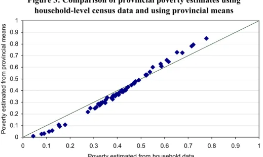
Figure 3 compares the provincial poverty estimates obtained from the semi-log model with household-level census data and provincial means from the census data. It reveals the same pattern of errors as Figure 2, in which the incidence of poverty is exaggerated for the poorest provinces and understated for the least poor provinces. As explained above, this is due to the change in sign of the curvature of the cumulative normal function when the incidence of poverty rises above 50 percent. On the other hand, the estimates in Figure 2 are noticeably less accurate, with many of the points lying more than 5 percentage points from the diagonal. Intuitively, the lower level of accuracy is due to the smaller amount of information used to generate the poverty estimates, since Figure 3 is based on provincial means of the census data rather than EA-level means. Mathematically, the lower level of accuracy is due to the fact that the variance in
23 household characteristics within provinces is greater than that within enumeration areas, so the error term in equation (4) is larger.
The margin of error in using census data aggregated to the provincial level may be too high for some uses. Nonetheless, census data aggregated to the provincial level may still be useful in ranking provinces by poverty rate. The average absolute error in ranking the 61 provinces using the aggregated data is 0.92, and only one province changes more than three places in the ranking when provincial means of the census data are used.
Figure 3: Comparison of provincial poverty estimates using household-level census data and using provincial means
0 0.1 0.2 0.3 0.4 0.5 0.6 0.7 0.8 0.9 1 0 0.1 0.2 0.3 0.4 0.5 0.6 0.7 0.8 0.9 1
Poverty estimated from household data
P o vert y est imat e d f
rom provincial means
Figure 3—Comparison of provincial poverty estimates using household level census data and using provincial means
24
4. SUMMARY AND DISCUSSION
This paper combines household expenditure survey data and census data to estimate the incidence of poverty for 61 provinces in Vietnam. The results confirm that poverty is greatest (over 60 percent) in the northern mountain regions along the border of China and Laos, followed by the provinces in the North Central Coast and Central Highlands. The least poor areas are the major cities (where less than 5 percent are poor) and the rural areas surrounding Ho Chi Minh City, followed by the intensively cultivated Red River Delta and Mekong Delta.
In addition, the paper explores the errors associated with using aggregated census data, since national statistics agencies in Vietnam and many other countries are often reluctant to release household-level census data. Our analytical results suggest that the use of aggregated data will underestimate the incidence of poverty when the rate is below 50 percent and overestimate it where the rate is above 50 percent. The magnitude of the error varies with the estimated incidence of poverty, being smallest when the poverty rate is close to zero, 50 percent, and 100 percent. Furthermore, the error is proportional to the variance in estimated per capita expenditure within the aggregated geographic units.
Empirical results using the Vietnam data indicate that, if census data are aggregated to the level of Census enumeration area (each of which has about 85 households), the errors in estimating the incidence of poverty are relatively small, averaging about 2 percentage points for national, regional, and provincial estimates of poverty. Ninety-eight percent of the provincial poverty estimates using EA-level census have errors of less than 5 percentage points. Not surprisingly, errors were larger when
25 the level of aggregation was greater. Using census data aggregated to the level of the province (of which there are 61 in Vietnam) resulted in errors of 3 to 4 percentage points, on average, with almost one-third of the provincial estimates being off by more than 5 percentage points. Using census data aggregated to the level of the region (nine regions were used in this study) was the least accurate, resulted in errors of around 4 percentage points, on average.
The study also compared the use of the semi-log regression model with that of the probit regression model. Using household census data, the incidence of poverty from the probit equation differed from that obtained from the semi-log equation by about 1.4 percentage points. Similarly, the use of the probit model added one percentage point in error when using the aggregated census data.
What are the implications of these results for other studies that combine household survey data and census data to produce high-resolution poverty maps?
Clearly, the best option is to carry out the analysis with household-level census data. Not only does this generate more accurate estimates of the incidence of poverty (P0), but it
allows the estimation of various other measures of poverty (P1 and P2) and inequality as
well as estimates of standard errors of these measures, none of which are possible with aggregated census data. Once the census data are aggregated, information about the variability of expenditure across households within the unit of aggregation is lost,
information necessary for estimating inequality and the higher-order measures of poverty (see Hentschel et al, 2000 and Elbers et al, 2001).
26 At the same time, the results presented in this paper suggest that if household-level census data are not available, as is often the case, it is possible to generate
reasonably accurate estimates of the incidence of poverty using aggregated census data. The errors associated with aggregation are more likely to be acceptable if the level of aggregation of the census data is relatively low, such as at the district or enumeration area. Furthermore,even highly aggregated census data can be used to rank provinces by poverty rate relatively accurately.
If aggregate census data are used to generate poverty estimates, the results in this paper provide information on the likely size and direction of bias. For example,
household-level data from a sub-sample of the census or a household survey could be used to estimate the variance in per capita expenditure which could be used in equation (4) to estimate the error associated with using aggregate census data.
Overall, these results suggest that, in some cases, high-resolution maps of the spatial patterns in poverty can be generated even in countries for which only aggregated census data are available. Such maps can contribute to efforts in these countries to alleviate poverty through geographically targeted policies and programs.
27
REFERENCES
Baker, J. and Grosh, M., 1994, “Poverty reduction through geographic targeting: how well does it work?’ World Development, Vol. 22, No. 7: 983-995
Bigman, D., Dercon, S., Guillaume, D., and Lambotte, M., 2000, “Community targeting for poverty reduction in Burkina Faso”, in D. Bigman and H. Fofack (eds),
Geographic Targeting for Poverty Alleviation: Methodology and Applications,
Washington DC: World Bank Regional and Sectoral Studies
Bigman, D. and Fofack, H, 2000, Geographic Targeting for Poverty Alleviation:
Methodology and Applications, Washington DC: World Bank Regional and
Sectoral Studies
Cornia, G., and Stewart, F., 1995, “Two errors of targeting” in Van de Walle, D. and Nead. K. (eds.), Public Spending and the Poor, Baltimore and London: John Hopkins University Press.
Elbers, C., Lanjouw, J. and Lanjouw, P., 2001, “Welfare in villages and towns: micro-level estimation of poverty and inequality”, The World Bank. Washington, D.C. Henninger, N. and M. Snel. 2002. Where are the poor? Experiences with the
development and use of poverty maps. World Resources Institute (Washington,
D.C.) and UNEP/GRID-Arendal (Arendal, Norway).
Hentschel, J., Lanjouw, J., Lanjouw, P. and Poggi, J., 2000, “Combining census and survey data to trace the spatial dimensions of poverty: a case study of Ecuador”,
World Bank Economic Review, Vol. 14, No. 1: 147-65
Minot, N., 1998, “Generating disaggregated poverty maps: An application to Viet Nam”. Markets and Structural Studies Division, Discussion Paper No. 25.. International Food Policy Research Institute, Washington, D.C.
Minot, N., 2000, “Generating disaggregated poverty maps: an application to Vietnam”
World Development, Vol. 28, No. 2: 319-331
Poverty Working Group, 1999, Vietnam: Attacking Poverty, A Joint Report of the Government of Vietnam-Donor-NGO Poverty Working Group presented to the Consultative Group Meeting for Vietnam
28 Ravallion, M. , “Poverty Comparisons”, Living Standard Measurement Working Paper
No. 88, Washington DC: World Bank
Statistics South Africa and the World Bank, 2000, ‘Is census income an adequate measure of household welfare: combining census and survey data to construct a poverty map of South Africa”, Mimeo
World Bank, 1999, Viet Nam: Poverty assessment and strategy. The World Bank. Washington, D.C.
World Bank, 2000, Panama Poverty Assessment: Priorities and Strategies for Poverty
29
Appendix A: Derivation of error associated with using aggregate census data
This appendix derives an expression that describes the error associated with using aggregate census data instead of household-level census data in the second step of a poverty mapping analysis. We start with the second-order Taylor expansion:
) ( '' ) ( 2 1 ) ( ' ) ( ) ( ) ( 2 0 0 1 0 0 1 0 1 f x x x f x x x f x x f ≅ + − + −
If we duplicate this expression for N values of x, labeled x1..xN, and take the sum of the N
equations, we get the following:
∑
∑
∑
∑
≅ + − + − i i i i i i i f x x x f x x x f x x f ( ) ''( ) 2 1 ) ( ' ) ( ) ( ) ( 2 0 0 0 0 0Dividing by N and setting the reference point (x0) equal to the mean value of x (x), the
result is:
( )
∑
∑
∑
≅ + − + − i i i i i i x x f x N x f x x N x f x f N 2 ( ) ''( ) 1 ) ( ' ) ( 1 ) ( 1 2But since the sum of deviations from the mean is zero, the second term on the right side drops out. Furthermore, the third term on the right side can be expressed in terms of the variance of x.
( )
var( ) ''( ) 2 1 ) ( 1 x f x x f x f N i i i + ≅∑
This equation gives us the approximate relationship between the average of a function (on the left side) and the function of an average (first term on the right side) In order to apply this general equation to the specific problem of poverty mapping with aggregate census data, we replace f(.) with Φ(.), the cumulative normal distribution, and
30 we replace xi with (µ- XiC ß)/σ, the normalized difference between the poverty line (µ)
and the estimated per capita expenditure for household i (XiCß). The result is:
− Φ − + − Φ ≅ − Φ
∑
∑
∑
i C i C i i C i i C i X N X X N X N σ β µ σ β µ σ β µ σ β µ 1 '' var 2 1 1 1If we assume that the adopted poverty line (µ) and the regression parameters (ß and σ) are constant across the unit of aggregation of the census data, which will normally be the case11, then the first term on the right-hand side can be rewritten as follows:
− Φ − + − Φ ≅ − Φ
∑
µ σ β µ σ β µ σ iCβ µ σ Cβ C i C i X X X X N 2var '' 1 1The interpretation of this equation is provided in Section 3.2 of the paper.
11Typically, the regression analysis is carried out for urban and rural sectors or for each stratum of the
household expenditure survey, so there are between 2 and 20 areas over which the regression parameters are constant. Similarly, the number of estimated poverty lines is usually relatively small (less than 20). By contrast, aggregated census data is often at the level of the district or enumeration area, of which there are generally more than 100. Thus, within a unit of aggregation, the poverty line and the regression parameters will, in most cases, be constant.
31
MSSD DISCUSSION PAPERS
1. Foodgrain Market Integration Under Market Reforms in Egypt, May 1994 by
Francesco Goletti, Ousmane Badiane, and Jayashree Sil.
2. Agricultural Market Reforms in Egypt: Initial Adjustments in Local Output
Markets, November 1994 by Ousmane Badiane.
3. Agricultural Market Reforms in Egypt: Initial Adjustments in Local Input
Markets, November 1994 by Francesco Goletti.
4. Agricultural Input Market Reforms: A Review of Selected Literature, June 1995
by Francesco Goletti and Anna Alfano.
5. The Development of Maize Seed Markets in Sub-Saharan Africa, September 1995
by Joseph Rusike.
6. Methods for Agricultural Input Market Reform Research: A Tool Kit of
Techniques, December 1995 by Francesco Goletti and Kumaresan Govindan.
7. Agricultural Transformation: The Key to Broad Based Growth and Poverty
Alleviation in Sub-Saharan Africa, December 1995 by Christopher Delgado.
8. The Impact of the CFA Devaluation on Cereal Markets in Selected CMA/WCA
Member Countries, February 1996 by Ousmane Badiane.
9. Smallholder Dairying Under Transactions Costs in East Africa, December 1996
by Steven Staal, Christopher Delgado, and Charles Nicholson.
10. Reforming and Promoting Local Agricultural Markets: A Research Approach,
February 1997 by Ousmane Badiane and Ernst-August Nuppenau.
11. Market Integration and the Long Run Adjustment of Local Markets to Changes in
Trade and Exchange Rate Regimes: Options For Market Reform and Promotion
Policies, February 1997 by Ousmane Badiane.
12. The Response of Local Maize Prices to the 1983 Currency Devaluation in Ghana,
32
MSSD DISCUSSION PAPERS
13. The Sequencing of Agricultural Market Reforms in Malawi, February 1997 by Mylène
Kherallah and Kumaresan Govindan.
14. Rice Markets, Agricultural Growth, and Policy Options in Vietnam, April 1997 by
Francesco Goletti and Nicholas Minot.
15. Marketing Constraints on Rice Exports from Vietnam, June 1997 by Francesco
Goletti, Nicholas Minot, and Philippe Berry.
16. A Sluggish Demand Could be as Potent as Technological Progress in Creating
Surplus in Staple Production: The Case of Bangladesh, June 1997 by Raisuddin
Ahmed.
17. Liberalisation et Competitivite de la Filiere Arachidiere au Senegal, October
1997 by Ousmane Badiane.
18. Changing Fish Trade and Demand Patterns in Developing Countries and Their
Significance for Policy Research, October 1997 by Christopher Delgado and
Claude Courbois.
19. The Impact of Livestock and Fisheries on Food Availability and Demand in 2020,
October 1997 by Christopher Delgado, Pierre Crosson, and Claude Courbois.
20. Rural Economy and Farm Income Diversification in Developing Countries,
October 1997 by Christopher Delgado and Ammar Siamwalla.
21. Global Food Demand and the Contribution of Livestock as We Enter the New
Millenium, February 1998 by Christopher L. Delgado, Claude B. Courbois, and
Mark W. Rosegrant.
22. Marketing Policy Reform and Competitiveness: Why Integration and Arbitrage
Costs Matter, March 1998 by Ousmane Badiane.
23. Returns to Social Capital among Traders, July 1998 by Marcel Fafchamps and
Bart Minten.
24. Relationships and Traders in Madagascar, July 1998 by M. Fafchamps and B.
33
MSSD DISCUSSION PAPERS
25. GeneratingDisaggregated Poverty Maps: An application to Viet Nam, October
1998 by Nicholas Minot.
26. Infrastructure, Market Access, and Agricultural Prices: Evidence from
Madagascar, March 1999 by Bart Minten.
27. Property Rights in a Flea Market Economy, March 1999 by Marcel Fafchamps
and Bart Minten.
28. The Growing Place of Livestock Products in World Food in the Twenty-First
Century, March 1999 by Christopher L. Delgado, Mark W. Rosegrant, Henning
Steinfeld, Simeon Ehui, and Claude Courbois.
29. The Impact of Postharvest Research, April 1999 by Francesco Goletti and
Christiane Wolff.
30. Agricultural Diversification and Rural Industrialization as a Strategy for Rural
Income Growth and Poverty Reduction in Indochina and Myanmar, June 1999 by
Francesco Goletti.
31. Transaction Costs and Market Institutions: Grain Brokers in Ethiopia, October
1999 by Eleni Z. Gabre-Madhin.
32. Adjustment of Wheat Production to Market reform in Egypt, October 1999 by
Mylene Kherallah, Nicholas Minot and Peter Gruhn.
33. Rural Growth Linkages in the Eastern Cape Province of South Africa, October
1999 by Simphiwe Ngqangweni.
34. Accelerating Africa’s Structural Transformation: Lessons from East Asia,
October 1999, by Eleni Z. Gabre-Madhin and Bruce F. Johnston.
35. Agroindustrialization Through Institutional Innovation: Transactions Costs,
Cooperatives and Milk-Market Development in the Ethiopian Highlands,
November 1999 by Garth Holloway, Charles Nicholson, Christopher Delgado, Steven Staal and Simeon Ehui.
36. Effect of Transaction Costs on Supply Response and Marketed Surplus:
Simulations Using Non-Separable Household Models, October 1999 by Nicholas
34
MSSD DISCUSSION PAPERS
37. An Empirical Investigation of Short and Long-run Agricultural Wage Formation
in Ghana, November 1999 by Awudu Abdulai and Christopher Delgado.
38. Economy-Wide Impacts of Technological Change in the Agro-food Production
and Processing Sectors in Sub-Saharan Africa, November 1999 by Simeon Ehui
and Christopher Delgado.
39. Of Markets and Middlemen: The Role of Brokers in Ethiopia, November 1999 by
Eleni Z. Gabre-Madhin.
40. Fertilizer Market Reform and the Determinants of Fertilizer Use in Benin and
Malawi, October 2000 by Nicholas Minot, Mylene Kherallah, Philippe Berry.
41. The New Institutional Economics: Applications for Agricultural Policy Research
in Developing Countries, June 2001 by Mylene Kherallah and Johann Kirsten.
42. The Spatial Distribution of Poverty in Vietnam and the Potential for Targeting,
March 2002 by Nicholas Minot and Bob Baulch.
43. Bumper Crops, Producer Incentives and Persistent Poverty: Implications for
Food Aid Programs in Bangladesh, March 2002 by Paul Dorosh, Quazi
Shahabuddin, M. Abdul Aziz and Naser Farid.
44. Dynamics of Agricultural Wage and Rice Price in Bangladesh: A Re-examination,
March 2002 by Shahidur Rashid.
45. Micro Lending for Small Farmers in Bangladesh: Does it Affect Farm
Households’ Land Allocation Decision?, September 2002 by Shahidur Rashid,
Manohar Sharma, and Manfred Zeller.
46. Rice Price Stabilization in Bangladesh: An Analysis of Policy Options, October
2002 by Paul Dorosh and Quazi Shahabuddin
47. Comparative Advantage in Bangladesh Crop Production, October 2002 by Quazi
Shahabuddin and Paul Dorosh.
48. Impact of Global Cotton Markets on Rural Poverty in Benin, November 2002 by