Poverty traps, aid, and growth

Poverty Traps, Aid, and Growth

Aart Kraay and Claudio Raddatz The World Bank

World Bank Policy Research Working Paper 3631, June 2005

The Policy Research Working Paper Series disseminates the findings of work in progress to encourage the exchange of ideas about development issues. An objective of the series is to get the findings out quickly, even if the presentations are less than fully polished. The papers carry the names of the authors and should be cited accordingly. The findings, interpretations, and conclusions expressed in this paper are entirely those of the authors. They do not necessarily represent the view of the World Bank, its Executive Directors, or the countries they represent. Policy Research Working Papers are available online at http://econ.worldbank.org.

1818 H Street N.W., Washington, DC 20433, akraay@worldbank.org, craddatz@worldbank.org. This paper was prepared as a background paper for the 2005 Global Monitoring Report. We would like to thank Andy Berg, Carlos Leite, and Zia Qureshi for helpful discussions, and Ana Margarida Fernandes for generously sharing her data on Colombian plants.

WPS3631

Public Disclosure Authorized

Public Disclosure Authorized

Public Disclosure Authorized

Abstract

This paper examines the empirical evidence in support of the poverty trap view of underdevelopment. We calibrate simple aggregate growth models in which poverty traps can arise due to either low saving or low technology at low levels of development. We then use these models to assess the empirical relevance of poverty traps and their consequences for policy. We find little evidence of the existence of poverty traps based on these two broad mechanisms. When put to the task of explaining the persistence of low income in African countries, the models require either unreasonable values for key parameters, or else generate counterfactual predictions regarding the relations between key variables. These results call into question the view that a large scaling-up of aid to the poorest countries is a necessary condition for sharp and sustained increases in growth.

1. Introduction

The idea of poverty traps has captured the imagination of development economists and policymakers alike for many years. It is not hard to see why. There are many very plausible self-reinforcing mechanisms through which countries (or individuals) who start out poor are likely to remain poor. There is also an abundance of empirical evidence that most countries that were relatively and absolutely poor in the middle of the 20th century remain so today. Recent calls for across-the-board debt relief and a major scaling up of aid to help poor countries achieve the Millennium Development Goals have been significantly influenced by the idea that these countries are stuck in poverty traps and major pushes are required to break free of these traps (see for example Sachs et. al. (2004, 2005)).

In this paper we examine the empirical evidence in support of the poverty trap view of underdevelopment. We do this by calibrating specific theoretical macroeconomic models of poverty traps in order to assess both their empirical relevance and their consequences for policy. We focus on two specific mechanisms generating poverty traps: low saving and low levels of productivity at low levels of development. It is not hard to see how either of these can generate a poverty trap. If either saving or productivity is low at low levels of development, investment will be low and countries will converge to an equilibrium with low capital and output per capita. If over some range of income levels saving and/or productivity increase sharply, then if countries can get to this point they might also be able to converge to an equilibrium with high capital and output per capita. We focus on these mechanisms because they capture some of the most popular explanations for the existence of poverty traps, and because they are often used as an explicit motivation for foreign aid to help countries escape from poverty traps.

We find little evidence of the existence of poverty traps based on these two broad mechanisms. Admittedly, both mechanisms can theoretically generate poverty traps, or at least very persistent poverty. However, when put to the task of explaining the persistence of low income in African countries, the models require either unreasonable values for key parameters, or else generate counterfactual predictions regarding the relations between key variables. These results call into question the view that a large scaling-up of aid to the poorest countries will result in sharp and sustained increases in growth.

In the case of the savings mechanism, generating a poverty trap consistent with the experience of poor African countries with a simple Solow growth model with a variable saving rate requires this rate to be a steep s-shaped function of capital per capita. Savings should be low

at low levels of capital per worker, increase significantly at some intermediate levels and level off at high levels. The actual relation between the saving rate and capital per capita observed in the data is far from meeting these conditions. Instead, saving rates seem to be increasing at low levels of capital per worker, flat at intermediate levels and increasing again at high levels.

The inability of the savings based explanation to account for the experience of African countries is not the result of the exogenous behavior of the saving rate imposed by the Solow model. Building on standard explanations for the inability of countries to save at low levels of income, we also calibrate a model of subsistence consumption with optimizing agents. We find that for this model to account for a country’s persistent low level of income, the country must be very close to the level of subsistence consumption. Given the high dispersion of consumption across countries in Sub-Saharan Africa, accounting for slow growth in these countries requires us to argue that subsistence consumption levels are country-specific and vary a lot from one country to the next. If we instead assume a common level of subsistence consumption, the model predicts that most African countries should be rapidly converging to their stable equilibrium. The model also predicts that, by rapidly relaxing the constraints that subsistence consumption imposes on capital accumulation, aid should quickly have an important impact on growth and savings. We perform a series of very simple regressions and review the existing literature to demonstrate that this prediction is not borne out by the data.

Technology based explanations of poverty traps based on aggregate models do not fare better. In a Solow framework similar to the one discussed above for the saving rate, we find that the relation between TFP and aggregate variables found in the data is significantly different than the s-shaped pattern required to induce a poverty trap. We also focus on a broad class of models of optimizing agents facing a technology with increasing returns that are external to the firm. Within these models, we show that the existence of an stable poverty trap equilibrium requires the external increasing returns to be sufficiently large relative to the diminishing returns in the production function. We find that such strong increasing returns are inconsistent with existing estimates from the vast empirical literature on the estimation of production functions, as well as some simple estimates of our own.

Based on the previous findings, we conclude that simple aggregate models of poverty traps we consider are not promising candidates to account for the experience of African countries. To the extent that these models capture some important features of reality, the results suggest that a large expansion of aid is not a necessary condition to improve the prospects of these countries. The available data suggest that, at least at the aggregate level there is not enough non-convexity

in underlying fundamentals to expect that large-scale increases in aid will be proportionately more effective than more moderate amounts of assistance. This does not mean that increasing aid to Africa (or other poor countries) is a bad idea. Rather, it suggests to us that we should not expect any disproportionate growth effects of large-scale aid.

We do not claim that this paper provides comprehensive coverage of the possible mechanisms of poverty traps, and the simple aggregate models we consider here are unable to capture some possible mechanisms mentioned in the literature. A significant fraction of this literature is based on highly stylized models, and on non-convexities at the micro-level, which are not easily amenable to calibration using aggregate data. Also, we face the standard trade-off of breadth versus depth. We have chosen to analyze a set of broad models that rely on aggregate mechanisms without delving deeply into the possible micro-mechanisms that lie behind our aggregate relations. A possible alternative approach would be to take seriously a specific micro-mechanism of poverty traps and make an effort to calibrate it using micro and macro data. Nevertheless, we consider that there are some important general lessons that can be derived from our analysis. The mechanisms that we analyze are usually mentioned in the discussion on poverty traps, and the models we use are standard in the growth literature. Also, under some conditions these models can be understood as reduced form representations of the underlying micro-mechanism.

It is important to notice that by using a representative-agent model in our analysis, we are implicitly assuming perfect factor markets, which leaves aside an important set of microeconomic models of poverty traps based on credit and labor market imperfections that result

in apparently large TFP differences across countries.1 However, despite their importance, these

types of models do not speak directly to the issue of whether large across-the-board increases in aid are likely to move poor countries out of poverty. The reason is that the low aggregate productivity associated with these types of models is related to distributional problems. A redistribution of income from rich to poor people within a country could increase measured aggregate TFP without an increase in aid. Also, modest increases in aid could have large productivity results if properly targeted, while large increases could have no effect on measured aggregate TFP if they benefit those that have already moved out of the poverty trap. Therefore, in

1

the aid context, these models speak more directly to the importance of aid targeting than to any non-linear growth effects of aid.

The rest of this paper is organized as follows. In the next section we review some of the existing evidence on poverty traps. In Section 3 we discuss saving-based poverty traps, and consider the role of foreign aid in helping countries to escape from such traps. In Section 4 we consider the evidence for technology-based poverty traps. Section 5 concludes.

2. Existing Empirical Evidence on Poverty Traps

In this section we briefly review some of the few existing empirical studies relating to poverty traps. One strand of the literature provides very reduced-form evidence based on cross-country data. If poverty traps are an important feature of growth dynamics, then over time one would expect to observe a bimodal distribution of per capita income, with a group of poor countries clustered around the low-level poverty-trap equilibrium, and a group of rich countries clustered around the high equilibrium (see Azariadis and Stachurski (2004) for details). In a series of papers Quah (1993a, 1993b, 1996, 1997) has used non-parametric methods to estimate the evolution of the distribution of per capita income across countries. His results suggest the emergence of such a bimodal distribution of income. This finding is supported by a recent paper by Bloom, Canning, and Sevilla (2003) which provides evidence that, after controlling for countries’ geographic characteristics, the evolution of income across countries is consistent with a bimodal ergodic distribution. There is some controversy, however, regarding the bimodality of the long-run income distribution: Kremer, Stock, and Onatski (2001) argue that the dynamics of the world income distribution is better characterized by a prolonged transition, during which inequality may increase, towards a single-peaked long-run distribution. A similar result is obtained in Azariadis and Stachurski (2004b), who uses a parametric model of income dynamics derived from an explicit growth model based on Azariadis and Drazen (1990). They also find that the long-run income distribution is unimodal, but that bimodality will appear during the transition. The last two papers are therefore only partly consistent with the idea of poverty traps,

in the sense that income disparities may be very persistent and appear as poverty traps, but

eventually, all countries would converge to the same equilibrium.2

On a different front, a recent paper by Feyrer (2003) raises some questions about the underlying causes behind the finding of bimodal distributions. The paper suggests that the bimodality of income distribution found by Quah results from a bimodal distribution of TFP, and therefore from productivity differences. Whether the bimodality of TFP results purely from increasing returns or from barriers to technology adoption may have different implications about the validity of the poverty traps story to account for the bimodality of the income distribution.

At a deeper level, the main drawback of this body of evidence is that, for the most part, their empirical analysis of the evolution of income distribution is non-parametric and unrelated to any underlying growth model, in particular, to any poverty trap story. The evidence is therefore at most consistent with a model of poverty traps. It does not provide proof of the validity of these models, nor does it address whether the magnitudes of the underlying mechanisms are empirically plausible. An exception is the paper by Azariadis and Stachurski (2004b) cited above, which assume the presence of increasing returns external to the firm as the underlying cause of non-convexities. While this model can generate bimodality during the transition, the parameters estimated for the production function are somewhat unreasonable, suggesting incredibly large degrees of increasing returns at some levels of income. As we will discuss in section 4, these levels of increasing returns are not supported by the data.

If poverty traps are important, one would expect also to occasionally see growth spurts as countries manage to escape from such traps. In a recent paper, Hausmann, Pritchett, and Rodrik (2004) empirically examine such “growth accelerations”, which they define as increases in growth of at least two percentage points that are sustained for at least eight years. They find that there are surprisingly many such accelerations, and that while they are in general quite difficult to predict, it is the case that they are more likely to occur in poorer countries. However, as in the previous case, this evidence is merely consistent with escapes from poverty traps and it is not conclusive. As the authors note, the standard dynamics of convergence in a growth model with shocks would also suggest that large jumps in growth rates are more likely in poor countries than in rich countries.

2 _{Of course, as pointed out by Quah (2001) the distinction whether poor countries are expected to}

Overall, this reduced-form cross-country evidence is at most suggestive of the existence of poverty traps, but it is hardly conclusive. Moreover, this type of evidence tells us little about the specific mechanisms generating the poverty trap or the policy interventions required to escape from that poverty trap. More useful in this respect is a line of microeconometric evidence that focuses on finding direct evidence of the mechanisms underlying specific models of poverty traps. For example, McKenzie and Woodruff (2004) use data from microenterprises in Mexico to search for evidence of poverty traps based on non-convexities in the production function. They take seriously the argument that poverty traps might exist if there are large fixed costs to starting a business. If capital markets are imperfect and potential entrepreneurs are credit-constrained by their lack of collateral, then a poverty trap can exist since individuals who start out with low wealth are unable to finance potentially profitable investments in new businesses. They find that the fixed costs involved in starting up a small enterprise in Mexico are typically very low, in some sectors less than half the monthly wage of a low-wage Mexican worker. They also find that the returns to capital are very high even at very low levels of the capital stock, and cannot reject the hypothesis that returns are decreasing over the entire range of observed capital stocks. They conclude that their evidence is not consistent with this particular mechanism of poverty traps.

In contrast, a number of papers have found microeconometric evidence of spillovers or other externalities that could form the basis of poverty traps. For example, Jalan and Ravallion (2004) argue for the existence of spatial or geographic poverty traps. In a panel of households from China, they find that consumption growth at the household level increases with the local availability of “geographical capital” understood as the availability of roads, the local level of literacy, etc. Their evidence suggests that these aggregate factors (at the local level) increase the returns to capital faced by households. However, the main focus of the paper is to determine the impact of locally aggregate variables on household growth. They do not spell out a feedback mechanism from household growth to the evolution of the geographical capital that could generate a poverty trap. A direct interpretation of their evidence is that it shows that the factors captured in the geographical capital are a constraint to household growth. If we assume that household growth feeds back into these variables, it might be possible to generate a poverty trap, but the degree of feedback necessary to induce such a trap is not specified. A different type of microeconometric evidence can be found in Lokshin and Ravallion (2004), who empirically estimate non-linear dynamics in household income in two transition economies. While they find that adjustment to income shocks is nonlinear, they find no evidence of non-convexities that would cause temporary adverse shocks to permanently lower household income, as would be the case in a variety of models of poverty traps.

Finally, two recent papers take a calibration approach to the study of poverty traps as we do here. Graham and Temple (2004) use a static two-sector variable-returns-to-scale model and show how, with minimal data requirements, it is possible to calibrate two steady-states for each country in the world. They then use these calibrations to document the contribution of the differences between these equilibria to cross-country income differences. Their model assumes that two different productive sectors co-exist within a country, a traditional sector (agriculture) producing under diminishing returns to all its factors, and a modern sector (non-agriculture) that exhibits increasing returns that are external to the firm. They find that, depending on the degree of increasing returns assumed for the non-agricultural sector, their model can account from between 15% and 60% of the observed inequality in income distribution across countries. The model however cannot account for the large differences in income observed between poor and rich countries. For extreme values of the increasing returns, the model predicts that output in the high equilibrium is about 3 times output in the low equilibrium, far below the fifty fold difference observed between the poorest and richest countries in the world. The model therefore can at most account for the difference between poor and middle income countries. The elegance and simplicity of the model, which allows it to determine the underlying alternative equilibrium for each country in the world with minor data requirements, comes at two costs. First, in the simplest version of the model the low equilibrium is unstable, so the authors have to resort to some ad-hoc assumptions about the presence of a fixed cost of switching sectors. Second, the model is static and focuses on the comparison of the different possible steady states of a country. So, the model is mute about how the equilibrium is selected for each country, and, most importantly, it does not allow us to analyze the dynamics of a country’s income, the impact of policy interventions, or the size or type of policies required to move a country away from its low equilibrium.

The second paper that adopts a calibration approach is Caucutt and Kumar (2004). They calibrate models with multiple equilibria that capture four main mechanisms: coordination failures, inappropriate mix of occupations, insufficient human capital accumulation, and political-economy considerations. They argue that while it is possible to find plausible parameter values that deliver multiple equilibria in these models, the existence of this multiplicity is also quite sensitive to small variations in these parameters. Based on this they caution against policy prescriptions for one-time interventions designed to jump countries from a bad equilibrium to a good one. Although both the methodological approach and the conclusions of this paper are quite similar to ours, our paper differs from theirs in two respects. First, we focus on different mechanisms generating poverty traps than they do. Second, and perhaps more important, Caucutt

existence of multiple equilibria are satisfied for plausible parameter values. They do not ask, as

we do, whether the magnitudes of the income differences attributable to these multiple equilibria are quantitatively reasonable.

3. Saving-Based Models of Poverty Traps

In this section of the paper we discuss one of the most popular models of poverty traps in which the source of the trap is inadequate saving at low levels of development. In these models, aid which augments domestic saving and finances accumulation can play a role in freeing countries from poverty traps. We first illustrate the basic mechanism using a very simple Solow growth model in which saving increases exogenously with the level of development. We next take seriously the main underlying theoretical mechanism why saving rates might increase with income: the influence of subsistence consumption. We present a Ramsey growth model with subsistence consumption and show that, while it does not have a stable low-level equilibrium like the poverty trap in the Solow model, it can exhibit poverty-trap-like features such as persistent slow growth for very long periods of time. Besides being usually cited as an explanation for poverty traps, the subsistence consumption model is representative of a class of models where multiple equilibria result only from the form of the preferences, and we speculate that the conclusions obtained in this case extend to other models of this class. Finally, we go to the data and ask whether there is any evidence that (a) saving rates exhibit the sort of nonlinear relationship with income required for the existence of a poverty trap, and (b) the historical relationship between aid, saving, and growth is consistent with escapes from poverty traps.

The Basic Mechanism

We begin by using the Solow growth model to illustrate a saving-based poverty trap and to perform some simple calibration exercises. With a Cobb-Douglas technology the familiar dynamics of the capital stock per worker in the Solow model are given by:

(1) k = s k( )⋅ ⋅A kα − + ⋅(n

δ

where k is the capital stock per capita, A is the exogenous level of technology, α is the output

elasticity of capital, and n and δ are population growth and depreciation rates. The key feature of

relax shortly. However, this assumption is very useful because it allows us to simply illustrate the existence of a saving-based poverty trap. In particular we allow the saving rate to be an exogenous function of the capital stock per capita, s(k), and assume that the saving rate is

constant at some low rate until a threshold value of the capital stock,

k

~

jumps to a constant higher rate, i.e.

(2)

( )

,

,

s

k

k

s k

s

k

k



≤



=



>



Figure 1 shows the familiar Solow diagram for this economy. There are two steady

states, indicated by kL and kH. The lower one can be thought of as a poverty trap, since if a

country starts out below kL, it will grow until it reaches the low steady state, and then remains

there forever. On the other hand, if a country starts out between

k

k

high saving rate, it will grow steadily until it reaches the high steady state. The basic intuition for the poverty trap is simple: at low levels of saving, investment is so low that it can only sustain a very small capital stock per capita.

We have calibrated Figure 1 so that it captures what we think are some key features of reality. We have drawn the low equilibrium at a capital stock per capita of $1500, which is approximately equal to the population-weighted average capital stock per capita in Sub-Saharan Africa. This is also roughly equal to output per capita in the region, implying a capital-output

ratio of around one. The capital-output ratio in the low steady state is given by

s

/(

n

+

δ

)

depreciation rate of 6% and population growth rate of 4%, this implies that the saving rate in the low steady state must be 10%, which is actually just a bit higher than the saving rate of 8% for

Sub-Saharan Africa as a whole.3 We then choose the level of technology, A, to ensure that the

steady state level of the capital stock at the low equilibrium, i.e.

1/(1 ) L L s A k n α

δ

$1500. For a benchmark value of α=0.5, this implies that A=1.22. We have drawn the high

steady state under the assumption that saving rates are twice that in the low steady state, but that there are no other changes in any of the parameters of the model. Since the ratio of the capital

3 _{Note that all calculations are done using PPP-adjusted data. Since the relative price of investment}

stocks in the high and low steady states is 1/(1 ) H H L L k s k s α −   =_{ }

  , for our benchmark value of α this

implies that the capital stock in the high steady state is four times that in the low steady state, at

H

k

Although Figure 1 shows that we can generate a growth model with a poverty trap that roughly matches Africa’s experience, it is important to note that the low poverty trap equilibrium exists only by assumption. Suppose for example that the point at which saving jumps to the higher rate occurs to the left of what is now shown as the poverty trap equilibrium. In this case, there would be no poverty trap, and a country starting out at the low capital stock would steadily grow until it reaches the high steady state. Similarly, if population growth or depreciation were slightly lower, the low equilibrium can also disappear as the diagonal line rotates downwards, leaving only a single stable high equilibrium. Moreover, if we were to introduce exogenous technical progress into the model, then the poverty trap equilibrium would also disappear,

provided that the threshold level of capital per capita

k

case, thanks to exogenous technical progress all countries will eventually cross this threshold and the poverty trap vanishes as all countries will have the high saving rates.

Suppose despite all this that the poverty trap exists, and that some countries find themselves stuck in it. How can aid help to break a country free of the poverty trap shown here? In the model, the reason countries are in a poverty trap is because their saving (and hence investment) rates are low. The role for aid in such a model is to augment saving sufficiently to allow the country to accumulate capital and grow to the point where the domestic saving rate jumps to the higher level. After the saving rate has increased, no further aid is required and the country grows steadily until it reaches the high equilibrium. To take a specific numerical example, suppose that we assume that the country in the low equilibrium receives a fixed fraction of its GDP in aid for a ten year period, and assume further that all of this aid is used to finance

capital accumulation.4 We can then calculate how large the aid inflow must be to ensure that the

country just reaches a per capita capital stock of

k

country will embark on sustained growth and eventually reach the high steady state without requiring further aid.

4

A ten-year period can be motivated by the time between now and 2015 when the Millenium Development Goals are supposed to be attained.

The results of this exercise are reported in Table 1. Clearly, the amount of aid required

depends on how far the threshold level of capital,

k

equilibrium. The columns of the table correspond to different values of

k

correspond to different assumptions on the degree of diminishing returns, α. For the benchmark

value of α=0.5, aid inflows ranging from 4 percent to 25 percent of GDP would be required for a

ten-year period in order to break the country out of the poverty trap. Obviously, the higher the threshold level of capital at which saving rates increase, the greater is the aid required. In

addition, the stronger are diminishing returns, i.e. the lower is α, the more aid is required.

This very simple example illustrates what we think are some of the main messages of the paper. First, while it is clearly possible for poverty traps to exist, the mere fact that saving increases with income is not sufficient for the existence of a poverty trap – it needs to do so in just the right way. As we will see shortly cross-country evidence is not very compelling that the required nonlinearities in saving rates exist. Second, even if a poverty trap does exist, the size of the policy intervention required to get countries out of poverty traps is very sensitive to the parameters of the specific model of poverty traps, in this case, the precise point at which saving

rates jump, as well as the extent of diminishing returns, α.

Subsistence Consumption

An important limitation of the example above is that we simply assumed that saving rates increase at some level of development. In a fully specified model, saving rates are endogenously determined by optimizing agents. The question therefore is what types of preferences can generate saving functions whose behavior is consistent with the existence of poverty traps. One important explanation offered in the literature is based on the existence of subsistence consumption (see Azariadis (1996), Ben-David (1998), Sachs (2004)). The idea behind this explanation is that poor households do not save because they have to use their income to meet basic consumptions needs, but once these needs are met households may save quite a lot of their income. We now present and calibrate a model that formalizes this intuition by explicitly introducing a minimum consumption level in the preferences of the representative consumer in an otherwise standard Ramsey model and deriving the optimal consumption and saving behavior

under these conditions.5 The model is closely related to Ben-David (1998), which analyzes the implications of a model with subsistence consumption under exogenous growth.

The representative household chooses a path for consumption to maximize its inter-temporal utility: (3) 0

( )

U

=

∫

u c e

dt

where c is the consumption per member of the household and the utility function is:

(4) 1

(

)

1

( )

1

c c

u c

θ

−

−

=

−

The minimum subsistence consumption level is captured by c . The representative

household is endowed with a constant returns production technology F K L( , ) and with an

endowment of labor that grows exogenously at rate

n

δ

Under these conditions, the evolution of the capital per worker is given by (5)

k

=

f k

( )

− − +

c

(

n

δ

)

k

where k denotes capital per worker, and f k( )=F K L( / ,1) represents the production function

in intensive form. The problem of the representative household is therefore

(6) 0

max

( )

. .

( )

(

)

U

u c e

dt

s t

k

f k

c

n

k

δ

=

=

− − +

∫

which is the standard Ramsey problem.

The first-order conditions of this problem are given by the following two differential equations:

5 _{This is of course not the only way to generate a saving rate that increases with the level of}

development. For example, Chakraborty (2004) develops a two-period overlapping generations growth model in which the probability of survival to the second period is endogenously determined as a function of public health care expenditures. The model exhibits an (unstable) low-level equilibrium in which the capital stock, income, and health spending are low. This in turn means that the probability of survival is low, and individuals rationally respond to this by saving less for their old age.

(7)

(

)

( '( )

)

( )

(

)

c c

c

f k

n

k

f k

c

n

k

δ ρ

θ

δ

−

=

− − −

=

− − +

The equations show that in contrast to the standard Ramsey model, c=c is also a stable

locus for the consumption dynamics. The implications can be seen in the phase diagram depicted in Figure 2. Compared with the standard Ramsey model, this model exhibits an additional unstable equilibrium at the point

( , )

c k

l

k

k c

,

( , )

c k

remain indefinitely at the subsistence level, and an economy that starts with capital below

k

maintain its consumption at the subsistence level and keep depleting its capital stock until eventually capital is exhausted and the economy ends up at zero consumption. Of course, even for the cases in which the high equilibrium of the standard Ramsey model is attained, the transitional dynamics of this model will differ substantially from those of the case with no subsistence consumption.

It is important to notice that this model is an example of a class of models where the multiplicity of equilibria results only from the form of the preferences. In general, the first order condition for the evolution of consumption in a Ramsey model corresponds to

( )( '( ) )

c=

σ

δ ρ

i

, where

σ

( )

c

substitution. It is clear from this equation, that, unless σ( )c =0, there is only one possible

equilibrium for the level of capital per worker, given by f’(k)=n+δ+ρ. So, the only way to obtain

multiple equilibria based only on the preferences is that they satisfy the condition

σ

( )

c

=

0

some positive value of c. Besides the Stone-Geary preferences, we are not aware of other standard specifications of the utility function that deliver this condition. We speculate therefore that the conclusions from this model apply to a much more general class of preference-based explanations for multiple equililibria. An important distinction between this model and the Solow model of the previous section is that the low equilibrium is unstable. As a result, countries cannot be “trapped” at this low equilibrium unless by some remarkable coincidence they begin just at the

low equilibrium.6 In other words, the model does not deliver a poverty trap. The reason is that, although the saving rate in the model is initially increasing with income, it does not have the s-shape (as a function of income) that is necessary to obtain multiple stable equilibria.

The failure of this model to generate a “standard” poverty trap shows how difficult it is to obtain such a trap as a result of optimizing behavior without assuming functional forms that are dangerously close to simply assuming that poverty traps exist. For example, Azariadis (1996) presents a OLG model of subsistence consumption similar to ours that delivers a poverty trap by assuming that the future level of subsistence consumption a step function of current wealth, hence making richer households effectively more patient. So, the way this model generates a poverty trap is by replacing the assumption of an shaped saving function with the assumption of an s-shaped discount factor.

Although our model does not deliver a standard poverty trap, its transitional dynamics may still generate something that looks like a poverty trap in the medium run. An economy that starts very close to the unstable equilibrium can exhibit consumption close to subsistence, low

saving rates, and low growth for a significant length of time.7 In order to take this possibility

seriously, we need to calibrate the key parameters of the model. We will assume that the

production function is Cobb-Douglas

f k

( )

=

Ak

, , , , andn

α δ

ρ

θ

α

which is larger than the value of 0.36 typically used for developed countries (e.g. Kehoe and Perri

6 _{So, this model cannot explain long run differences between countries unless we are willing to}

consider the zero consumption equilibrium as a possibility, or to assume that countries can remain indefinitely at the unstable intermediate equilibrium. Both alternatives are unsatisfactory. The zero consumption equilibrium is present in the standard Ramsey model, so it cannot be considered as the specific manner in which subsistence consumption induces a poverty trap. The only difference with the standard model in this respect is that in the model with subsistence consumption the zero equilibrium is the only possible steady state for an economy starting from very low levels of capital, which makes this equilibrium more likely. However, the model has the counterfactual implication that during the transition to the zero equilibrium an economy would exhibit negative saving rates. Also, it is hard to provide an economic intuition for an equilibrium with zero consumption in a model that explicitly includes subsistence consumption levels. Regarding the second possibility, by definition an unstable equilibrium cannot account for long run differences unless we are willing to assume the absence of any type of shocks.

(2002)). For the robustness analysis we will vary the capital share between the value of 0.4

considered by Coe, Helpman, and Hoffmaister (1995), and 0.6.8 The sum of the depreciation rate

δ

ρ

which is consistent with the standard quarterly value of 0.99 for the discount factor used in the RBC literature. Finally, the coefficient of risk-aversion (or the inverse of the intertemporal rate of

substitution)

θ

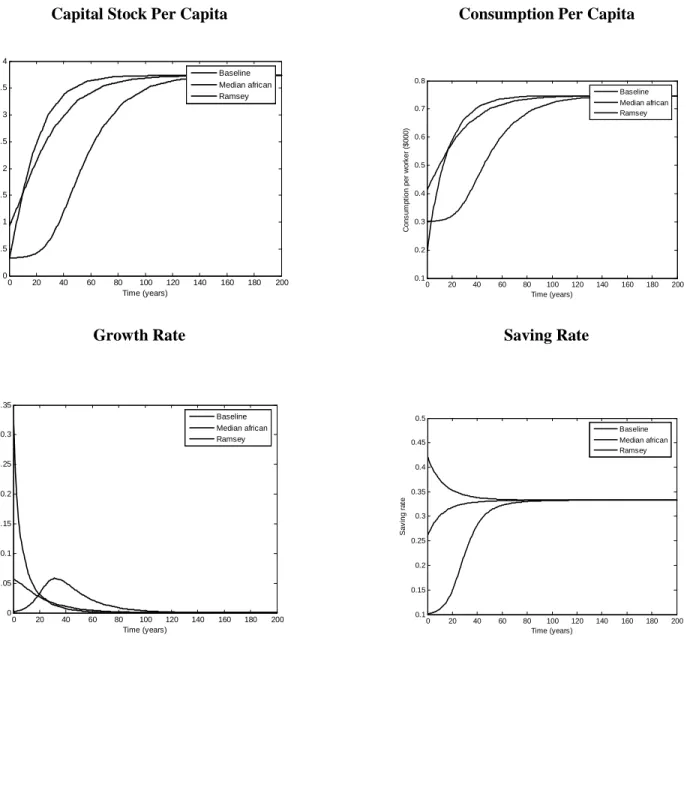
the unstable low equilibrium to the level of consumption per capita and capital per-worker of the poorest African country in 1996 (Democratic Republic of Congo with a consumption per capita of about $300 and capital per worker of $330). This seems like a reasonable lower bound for a subsistence level of consumption, and it is slightly smaller than the $300 in 1980 dollars computed by Ben-David (1998) as the least cost requirement for sustaining an individual’s minimum dietary needs.

The bottom panel of Figure 2 shows the c=0

i

and the k=0

i

locus in the (c, k) space for the benchmark economy. It also shows the stable manifold of the economy, which was computed numerically using the time-elimination method of Mulligan and Sala-i-Martin (1991). In this parameterization, the levels of consumption and capital per person at the high stable equilibrium correspond to $747 and $3,434 respectively. These levels are very low. So, a first quantitative implication of the calibration exercise is that the high equilibrium consistent with the poorest African country being at its subsistence level implies that, even after reaching the high equilibrium, per capita consumption will still be below that of the median African country, and well below that of middle income countries. Of course these magnitudes are sensitive to the specific parameterization, but, as will be shown below, taking them to more reasonable levels would require unlikely magnitudes for key parameters of the economy.

The effect of subsistence consumption on the pattern of growth for an economy that starts at an initial level of capital 1 percent above the low equilibrium is shown in Figure 3. For comparison, the figure also presents the evolution of capital per worker of an economy that starts

8

We cannot increase the value of

α

9 _{Standard values for}

θ

with a much higher level of capital equal to the one observed for the median African economy, and of a standard Ramsey economy with the same parameters. The top-left panel shows that the convergence of the capital stock to the steady state is significantly slower for the benchmark economy. The remaining panels show that the persistence of low levels of capital per worker for the benchmark economy also translates in a low and persistent level of consumption, growth, and saving rates. During the first 20 years, average consumption and capital per worker are $302 and $339, which are barely above the subsistence levels, the saving rate averages 11 percent, and the average growth rate is 0.5 percent. These are magnitudes that roughly fit the experience of poor countries.10

The previous figures suggest that persistent low output and slow capital accumulation observed in African countries could be explained by assuming that these countries are close to their subsistence level of consumption. While these economies would not be “trapped” in the usual sense because they would eventually reach the high equilibrium, they would nevertheless display slow growth performance for an extended period of time. Over time, however, the growth rate accelerates as subsistence consumption becomes less important, and finally the growth rate declines as the economy approaches the stable high equilibrium.

However, it is important to note that this poverty trap-like behavior is very sensitive to initial conditions. In particular, the length of time that low growth persists depends crucially on how close the initial level of capital is to the level corresponding to the low unstable equilibrium

l

k

steady state level of capital, assuming that the level of capital observed in low income countries is ten, one, one-tenth, and one-hundredth percent above the low unstable equilibrium. For the benchmark economy halving the distance to the steady state would take 54 years, as compared with just 12 years for the no-subsistence-consumption economy. However, a country that starts out 10 percent above the capital stock in the low equilibrium would take 41 years, and the median (un-weighted) African economy with a capital stock of $934 per capita would take only 17 years. In fact, it is apparent from the figures that, under the benchmark parameterization, the median African country should behave very similarly to the standard Ramsey economy. In other words,

10

Under this parameterization, the steady-state saving rate is about 33%. Although this magnitude is high, it can be easily reduced by increasing the discount rate

ρ

the existence of subsistence consumption should be practically irrelevant for the dynamics of the median African country, and even more so for countries richer than the median.

Table 2 also shows that the main quantitative implications of the model for growth near

subsistence levels of consumption are robust to the capital share

α

values for this parameter, and in each case re-calibrate the constant A to make the low unstable

equilibrium correspond to the values of consumption and capital observed for the poorest African

country.11 Although the level of the high equilibrium varies significantly, the pattern of

convergence looks similar in all three cases. In particular the times required to close half the gap

to the steady state are 59 years (

α

α

α

these differences with those obtained for economies that start at different distances from the low unstable equilibrium makes clear that the main determinant of the speed of convergence is the position of the initial conditions with respect to

k

In summary, the results from these simulations suggest that the model with subsistence consumption has the potential to generate something very similar to a poverty trap if we are willing to assume that poor African countries are very close to subsistence. However, the flipside of this assumption is that the median African country (and those above the median) should have very high saving rates and be close to its high long run equilibrium. One possible way of reconciling the predictions of the model with the data would be to assume that the subsistence consumption levels are country specific, so that most low income African countries are close to their own subsistence levels, but this would require us to argue that the subsistence consumption level can vary significantly across countries. The consumption of the poorest African country is one-third of the consumption of the median African country (PPP adjusted), and one-ninth of the consumption of the richest African country. Analogously, assuming a common but higher level of subsistence consumption, for example the consumption of the median African country, implies that half of the countries below that level would be drifting towards the zero consumption equilibrium, which is equally unappealing. These quantitative implications of the model suggest that the subsistence consumption story as a source of poverty traps has serious problems matching the data. Nevertheless, in what follows we will maintain the assumption that the persistence of

low levels of capital and consumption in poor countries results from the fact that they are close to the subsistence level, and ask how these countries can accelerate their escape from this situation.

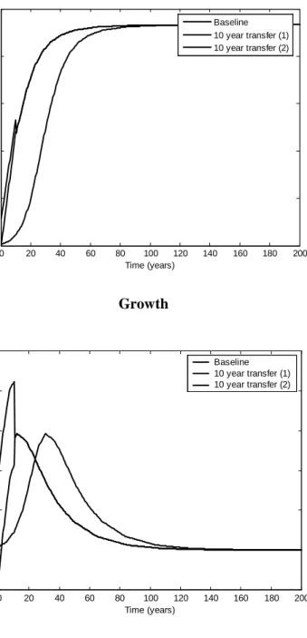
What is the role of aid in this economy? As in the previous example, aid that augments saving and domestic capital accumulation can bring the country toward the high steady state. Unlike in the previous example, however, in the absence of aid countries would eventually get to the high equilibrium on their own: all aid can do is accelerating this process. To get a sense of the magnitude of the interventions involved, we compute the annual aid transfer as a fraction of

GDP necessary to double and quadruple the initial level of capital in 10 years.12 Since saving

rates are determined endogenously, we also need to make assumptions on how aid is delivered. We consider two cases: (i) all transfers are exogenously directed to capital accumulation; (ii) the allocation of transfers is left to the recipient country, but they are perceived as permanent. These two cases give us a lower and upper bound for the more realistic case in which the transfers have some bias towards capital accumulation and are at least partially perceived as transitory.

The values obtained for the transfers are reported in Table 3 for the benchmark economy, the median African country, the Ramsey case, and for alternative values for the capital share (a=0.4, 0.6). For the benchmark economy, the annual transfer, as a fraction of GDP, required to double the capital per worker in a 10 year period is about 4 percent in the case in which all the transfer goes to capital accumulation and 9 percent if the transfer goes to income but is perceived as permanent (see columns (4) and (5)). As mentioned above, these two values represent a lower and upper bound for the actual transfers required assuming different degrees of anticipation of the end of the policy and biases towards capital accumulation. For this economy, doubling the initial capital stock would have taken almost 30 years if left to itself (see column (6)). Doubling the capital stock in 10 years therefore takes approximately 20 years from the development process of the baseline economy. Quadrupling the capital stock however requires a much larger effort, with transfers somewhere between 13 and 33 percent of GDP for 10 years.

Figure 4 shows the effects of aid on saving and growth in the first scenario of doubling the per capita capital stock. Remember that, in each graph, the two exercises represent a lower and upper bound for the true effects that should be observed. If we assume that the transfers are

12 _{For a very poor country with per capita income of $300 and a Gini coefficient of 40 to halve the}

headcount measure of poverty with a 1$ per day poverty line, income needs to roughly double (assuming an unchanged lognormal distribution of income). This in turn requires a quadrupling of the capital stock for our benchmark case of α=0.5.

fully invested, growth rates are higher on impact. Interestingly, for the case in which the transfers are perceived as permanent, we observe an initial decline in the growth rates. A permanent transfer of a fraction of GDP is in the model akin to an increase in TFP, which makes households consider that their old saving plan was excessive and review it by increasing consumption.

Going back to Table 3, we observe that the transfers required to double the capital stock for the median African country are higher than those obtained for the benchmark economy because it is closer to the steady state, and, therefore, diminishing returns are more important for the median country than for the country that is close to subsistence. For the median African country, quadrupling the capital would take it above the steady state level, so the exercise is

omitted. The last two rows show that the transfers are decreasing in

α

the lower bounds are about 5.4 percent for the low

α

The corresponding upper bounds are 15.5 and 6.2 percent respectively. In general, the bounds are

not very sensitive to reasonable changes in the elasticity of substitution

θ

There is a striking difference in the magnitude of required aid inflows in this example compared with the previous example based on the Solow model. To see this note that in Table 1 the case of attaining a threshold capital stock of $3000 in ten years corresponds to a doubling of the initial capital stock. In the Solow economy doubling the capital stock required 10.5 percent of

GDP in aid for 10 years for the benchmark value of α=0.5. In contrast, in Table 3 we see that

doubling the capital stock in the Ramsey economy with subsistence consumption requires only 3.9 percent of GDP in aid for the same capital share when aid goes directly to investment. The reason for this difference is that in the Solow economy, domestic saving by assumption remains constant at 10 percent of GDP and does not respond to the aid inflow. In contrast, in the subsistence economy model there is a very strong increase in saving. In the absence of aid saving rates would have averaged 10% of GDP in the first 10 years, while with aid saving rates increase sharply and average 16% of GDP during this period. This additional aid-induced domestic saving and investment has a strong effect on growth over and above the direct effects of aid.

In summary, the model could be used to rationalize the persistence of low levels of consumption and capital observed in low income African countries by assuming that they are close to the subsistence level, but this requires either to assume that there is significant variation in the levels of subsistence consumption across African countries or that half of these countries should exhibit high saving and growth rates. Also, taking the model seriously would imply that relatively modest transfers, well within the magnitudes we observe historically should have an

important effect on the performance of these countries. We next ask whether this has been the case empirically.

Empirical Assessment

In this sub-section we assess the empirical relevance of the saving based poverty trap models discussed above. We first ask whether the cross-sectional and time-series behaviour of saving is consistent with models of poverty traps. We then ask whether there is any evidence that in the past aid has helped countries to escape from saving-based poverty traps.

Consider first the nonlinear relationship between saving and the level of development that is required for a poverty trap to exist in the Solow model. In the left-hand panels of Figure 5 we plot the empirical counterpart of this relationship. In each panel we have gross domestic

investment rates on the vertical axis, and on the horizontal axis we have the capital stock.13 The

top panel plots data for all countries, the second only for low-income countries, and the third only for countries in Sub-Saharan Africa. In all these graphs we have fitted a third-order polynomial relationship to pick up any non-linearities that might be present in the data. These non-linearities do appear to be present in the cross-sectional relationship between investment rates and the level of development. In all three cases the patterns are broadly similar, with sharp increases in saving at very low capital stocks, then a fairly flat or even declining section, and then finally again an increasing section. Note however that these turning points occur at very different levels of the capital stock per capita, as the scale for the top graph is very different from the bottom two panels. In particular, for the low-income and Sub-Saharan Africa samples the turning points all occur at capital stocks less than $1500 per capita. Interestingly also, some of these nonlinearities are statistically significant: the quadratic and cubic terms in the first and third panels are statistically significant at the 5 percent level. At the same time, however, a visual inspection of the three graphs suggests that the shape of these nonlinearities is likely to be quite sensitive to extreme observations.

13 _{Throughout the paper we use data on investment rates as a proxy for saving rates. We do this}

mainly for reasons of data availability, as gross domestic investment rates are available for many more country-year observations than is gross national saving, reflecting gaps in data on current accounts. While many poor countries of course receive substantial recorded capital inflows, many also have substantial unrecorded capital outflows and so it is not obvious a priori the extent to which our findings are affected by this approximation.

Despite the presence and significance of these nonlinearities, the patterns shown in the left side of Figure 5 are not very promising for the poverty trap story. Recall that for the poverty trap story to work, we need to find low saving rates at low levels of development, and then a sharp increase over some intermediate range before leveling out at a high rate. This is just the opposite of what we see in the data. The consequences of these saving patterns for the Solow model are shown in the right panel of Figure 5. In the top panel the fact that saving rates are increasing and concave over the relevant range implies a unique stable equilibrium around a capital stock of $2000 per capita. For the low-income country sample we find a stable equilibrium around $4000 per capita and two unstable ones around $400 and $7000. For the Sub-Saharan Africa sample there is an unstable low equilibrium around $1000 and a stable high equilibrium at $6000. In none of these cases do we find a sufficiently S-shaped pattern in saving rates to generate a stable low-level equilibrium that might be thought of as a poverty trap, together with a stable high equilibrium that countries might be able to attain with appropriately large amounts of aid.

The bottom line here is that the cross-sectional patterns in saving rates do not appear to be particularly supportive of the existence of poverty traps. This is not because saving rates do not increase with the level of development. Rather the data suggest that they do not increase in the right nonlinear fashion required for the existence of a poverty trap.

We now turn to the empirical predictions of the Ramsey economy with subsistence consumption. A key prediction of this model, which can readily be seen from Figure 3, is that countries starting out near subsistence levels will eventually experience sharp increases in saving rates and sharp accelerations in growth as they reach a level of development where subsistence considerations are no longer important.

For the baseline calibrations a country starting off near subsistence will see its saving rates roughly double to 10 percent to 20 percent during the first 30 years, and growth will

accelerate from near zero to 5 percent per year.14 A first question to ask of the data is whether

jumps in saving rates of this magnitude are ever observed. In the top panel of Figure 6 we graph the change in decadal average investment rates between 1960 and 1990 on the vertical axis, and the initial log-level of per capita GDP in 1960 on the horizontal axis.

14 _{The jump in saving would be large even if we had a higher discount rate and therefore a lower}

The first thing to notice from this graph is that such large increases in saving rates, even over a 30-year period, are very unusual. Only three countries (Korea, Equatorial Guinea, and

Lesotho) have had such dramatic increases in investment rates.15 Even if we consider more

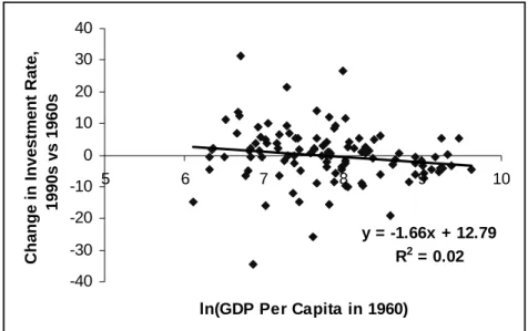
modest increases of 10 percent of GDP, we find only six more countries with increases in saving in the 10-20 percent range. This suggests that accelerations in saving of the magnitude suggested by subsistence consumption models are rare. Second, there is no obvious pattern in the data suggesting that accelerations in saving are more likely at low income levels. There is only a small and insignificant negative correlation between changes in saving and initial income. Moreover the large increases in saving above 10 percent of GDP are fairly evenly distributed among countries with per capita incomes ranging from about $600 to $3000 in 1960. In contrast, the benchmark calibration of the model implies that large increases in saving rates occur in a range much closer to subsistence levels. In fact, according to the calibration, the saving rate reaches 15% at about $424 of capital per capita (which according to the other parameters implies a level of income per capita of about $350). In the bottom panel of Figure 6 we ask whether large increases in saving tend to be accompanied by growth accelerations, as the model with poverty traps would suggest. There is a small and statistically insignificant relationship between changes in investment rates and changes in growth rates, contrary to the implication of the theory that saving and growth accelerations should go together.

Finally, we have seen that even fairly modest aid inflows can have very strong effects on growth in the subsistence economy model. This reflected both the direct effects of aid on capital accumulation, as well as the indirect effect of sharp increases in saving as aid makes the subsistence constraint less binding. In particular, the model predicts that aid should increase investment substantially, and that this in turn leads to a sharp increase in growth. Depending on the specific assumptions on the use of aid flows (whether they go completely to investment or to general expenditure) the increase in investment can be even more than one by one. At the very least, increases in investment should be roughly of the same magnitude than the aid flows (as a percentage of GDP). We have already seen a rather weak relation between investment and growth in Figure 6. In Figure 7 we explore the links between aid and investment. In the top panel we plot the relationship between aid as a fraction of GDP and the investment rate, both averaged over the 1990s. The first thing to note is that there have been cases of quite poor countries that have

15

In the case of Equatorial Guinea, large foreign investments in the oil sector are an important factor, while in Lesotho migrant workers’ remittances are an unusual contributing factor.

received very substantial aid inflows over 10-year periods, for example Guinea-Bissau at 17 percent of GDP, or Equatorial Guinea at 10 percent of GDP during the 1990s. Note also that these aid ratios have GDP adjusted for purchasing power parity in the denominators. Had we used

market exchange rates in the denominator the aid ratios would be much higher.16 In short,

however, there have been quite a few cases of poor countries receiving aid flows on the order of magnitude that our calibrations suggest would be required to get out of poverty traps.

Unfortunately, however, the poverty trap models also imply very large increases in investment should occur with aid. Yet the simple correlation between aid ratios and investment rates is weakly negative, both in levels (top panel) and in differences (bottom panel). The lack of a significant relation between aid and investment survives the inclusion of controls for policy, and holds among low-income countries and among Sub-Saharan African countries as well. A particularly extreme example is the case of Sao Tome and Principe, which is suppressed in the bottom panel because the observation is so extreme. Our data suggest that aid increased by 20% of GDP between the 1980s and the 1990s, yet investment rates fell by 5%.

None of these simple stylized facts should be especially surprising. Rodrik (2000) provides a careful analysis of episodes of “saving transitions” which he defines as increases of five percent or more in saving rates. He finds only 20 such episodes during the period 1960-1995. This suggests that escapes from poverty traps must be quite rare since their hallmark is a sharp increase in saving rates. It is also interesting to note that the saving transitions he identifies occur at a very wide range of per capita income levels, ranging from around $800 in China to over $6000 in Mauritius. It seems difficult to interpret the saving transitions occurring at high income levels as resulting from the escape from a poverty trap based on subsistence consumption simply because these countries are so rich that subsistence considerations matter little. Finally, Rodrik also documents that saving transitions do not tend to be accompanied by higher growth. Although these sharp increases in saving tend to persist for long periods of time, growth accelerates only for a relatively short period and quickly returns to its pre-transition level. This again seems inconsistent with the poverty trap story.

16 _{Which of the two is more appropriate? This depends on whether aid dollars are used to buy}

goods and services at international or at domestic prices. We are not aware of estimates of the division of aid along these lines. Here we report the PPP aid ratios simply to be conservative about the magnitude of

The other observation on the weak relationships between aid, investment and growth has been amply documented in a series of recent papers. Easterly (1999) finds that in only six of 88 countries for which data are available does aid raise investment at least one by one, and in only 17 countries the effect is positive and statistically significant. He also finds virtually no evidence that investment and growth are correlated within countries. For Africa in particular, Easterly and Dollar (1999) find that in none of 34 African countries aid increases savings at least one by one. Similarly, Devarajan, Easterly and Pack (2001, 2003) document that the effect of public investment on growth is not significantly different from zero, and that the effect of private investment on growth is significant only if Botswana is included in the sample. Based on this as well as a variety of micro evidence they conclude that the productivity of investment in Africa is extremely low.

In summary, while models of saving based poverty traps are quite intuitive and are frequently invoked as a motivation for aid, we fail to find any clear evidence in support of them. We have seen that there is little evidence in support of the nonlinearities in saving rates across countries required to generate poverty traps. We have also seen that there are very few instances of saving and growth accelerations that would be consistent with calibrated models of poverty traps. And finally, as many others have noted, there appears to be very little evidence that aid has an at least proportional effect on investment as these models would suggest. This is the case despite the fact that there have been quite a few episodes of countries receiving very large aid inflows that our calibrations suggest would be sufficient to break these countries out of poverty traps. Overall this evidence leads us to doubt the empirical relevance of saving-based models of poverty traps.

4. Technology-Based Models of Poverty Traps

We now turn to another popular argument for the existence of poverty traps: the idea that there are sharp increases in productivity once a certain threshold level of development is attained. This idea can be generated in a variety of models in which indivisibilities in production, externalities across firms, public infrastructure, and many other factors play a role. In this section we will not restrict ourselves to a particular mechanism generating the acceleration in productivity. Rather we will review some fairly general requirements for the existence of a

technology-based poverty trap, and then we will show that these requirements do not appear to hold in cross-country and firm-level data.

Theoretical mechanisms

To be consistent with perfect competition, theoretical models usually assume that increasing returns are external to the firm. As surveyed by Caballero and Lyons (1990), standard explanations for these economies of scale that are external to the firm but internal to the industry or country include advantages of within-industry specialization, agglomeration, indivisibilities and public intermediate inputs such as roads or other infrastructure. Some papers along these lines include Bryant (1983), Weil (1989) and Durlauf (1991) who introduce some form of externality in the production process, and Diamond (1982), Howitt (1985), and Howitt and McAfee (1988) who analyze models of search and matching with thick market externalities. Most of these models, however, are highly stylized and not amenable to calibration. Nevertheless, as mentioned above they share the common feature that the increasing returns are assumed to be external to the firm, so that, in a model of homogeneous firms, the technology of a representative firm j has the form:

(8) Yj = A E F K L( ) ( j, j)

where Yj, Kj, and Lj are the total output, capital, and labor of firm j, and A E( ), the scale

factor capturing total factor productivity, depends on a measure E of the average or aggregate level of activity. This dependence is taken as given by the atomistic firm. As usual, the function

F() is assumed to have constant returns to scale.

The crucial aspect of the specification above is the dependence of the scale factor on a measure of aggregate activity. Different models take different stances on what is the source of the external economies, which will determine what is the relevant variable that affects A. We will consider three possibilities. In the first specification, the scale factor depends on the average level of capital as captured in the capital per worker. This approach was introduced by Azariadis and Drazen (1990) in their model of threshold externalities, and, as noted by Barro and Sala-I-Martin (1991), it has the advantage of eliminating the scale effects that appear in models like the ones presented by Romer (1986) and Barro (1990). In the second specification, we assume that the scale factor depends on the aggregate level of output. This approach is similar to the one taken by Caballero and Lyons (1990, 1992, 1994), and Cooper and Haltiwanger (1996). Finally, we also consider the case in which the scale parameter depends on the aggregate level of capital, in the

specifications, we explore the restrictions that the existence of a stable low equilibrium imposes on the technological parameters and then we check whether these restrictions are actually borne out by the data.

The simplest specification for the case in which the scale factor depends on the level of capital per worker is the one considered by Azariadis and Drazen (1990), where there is a threshold level of capital at which there is a “technological jump”. That is

(9) A k( ) A if k k A A otherwise  _≤  = > 

The ability of a technology like this to account for the differences in income observed in low

income countries will of course depend on the threshold capital level

k

the analysis will be very similar to the one presented in Section 2. This is because, in the Solow model, the role of jumps in saving and jumps in technology are more or less interchangeable. In particular, all of the discussion in the first part of Section 2 can be re-interpreted as a story in which there is an exogenous improvement in productivity once capital per worker reaches a certain level. In this framework a poverty trap featuring low productivity can exist since for a given saving rate, low productivity means that investment is insufficient to generate sustained growth in the capital stock.

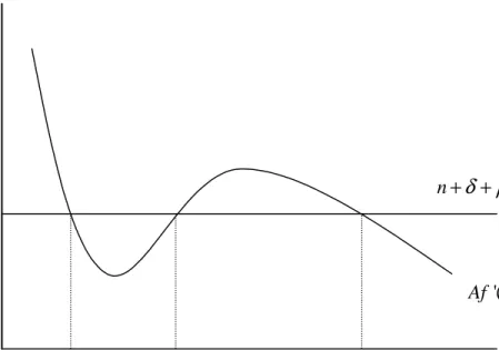
As we shall see shortly in the data, it seems difficult to find empirical evidence for such a discrete jump in the level of technology. However, it is possible to have a poverty trap with a less dramatic nonlinearity in technology. In fact, we can use the Ramsey economy of the previous section to ask what degree of increasing returns would be necessary over some range of the production function to obtain a stable low equilibrium corresponding to a poverty trap. Assume that TFP (A) is a function of aggregate capital stock per capita (A(k)) but that firms do not internalize the presence of the external effect in their production decisions. Under these assumptions, the two equations that govern the dynamics of the Ramsey economy are:

(10) 1 ( ( ) '( ) ) ( ) ( ) ( ) c A k f k n c k A k f k c n k

δ ρ

θ

δ

As in the standard Ramsey case, the equilibrium levels of capital are pinned down by the dynamics of consumption. In a steady state with no consumption growth the capital level has to

decreasing function of k respectively it is easy to see that it is possibl