Control of a Quadrotor Helicopter Using Visual Feedback

C o n t r o l of a Q u a d r o t o r H e l i c o p t e r U s i n g V i s u a l F e e d b a c k

Erdinc Altu~*, James P. Ostrowski*, Robert Mahony**

*GRASP Lab. University of Pennsylvania, Philadelphia, PA 19104, USA

**Dep. of Eng., Australian Nat. Uni., ACT 0200, Australia

E-mail" {erdinc, jpo}@grasp.cis.upenn.edu, [email protected]

A b s t r a c t

We present control methods for an autonomous four-rotor helicopter, called a quadrotor, using visual feedback as the primary sensor. The vision system uses a ground camera to estimate the pose (position and orientation) of the heli- copter. Two methods of control are studied one using a series of mode-based, feedback linearizing controllers, and the other using a backstepping-like control law. Various simulations of the model demonstrate the implementation of feedback linearization and the backstepping controllers. Finally, we present initial flight experiments where the helicopter is restricted to vertical and yaw motions.

1 I n t r o d u c t i o n

The purpose of this study is to explore the control methodologies that will make an unmanned aerial vehicle (UAV) autonomous. An autonomous UAV will be suit- able for applications like search and rescue, surveillance and remote inspection. Rotary wing aerial vehicles have distinct advantages over conventional fixed wing aircrafts on surveillance and inspection tasks, since they can take- off/ land in limited spaces and easily hover above the

target. A q u a d r o t o r is a four rotor helicopter. One

example is shown in Figure 1. The idea of using four rotors is not new. A full-scale four-rotor helicopter was built by De Bothezat in 1921 [11. Other examples are the Mesicopter [21 and Hoverbot [3]. Also, related models for controlling the VTOL aircraft are studied by Hauser et al [41 and in [51. Helicopters are dynamically unsta- ble and therefore suitable control methods are needed to make them stable. Although unstable dynamics is not de- sirable, it is good for agility. The instability comes from the changing helicopter parameters and the disturbances such as wind.

A quadrotor helicopter is controlled by varying the rotor speeds, thereby changing the lift forces. It is an under- actuated, dynamic vehicle with four input forces and six output coordinates. One of the advantages of using a multi-rotor helicopter is the increased payload capacity. It has more lift therefore heavier weights can be carried. Quadrotors are highly maneuverable, which enables ver- tical take-off/landing, as well as flying into hard to reach areas. Disadvantages are the increased helicopter weight

and increased energy consumption due to the extra mo-

tors. Since it is controlled with rotor-speed changes, it is more suitable to electric motors, and large helicopter engines which have slow response may not be satisfactory without a proper gear-box system.

The main concentration of this study is using non-linear control techniques to stabilize and perform output track- ing control of a helicopter. In Section 2 the helicopter

model and dynamics of quad-rotor is described. The

equation of motion of a simplified quadrotor is given here. Feedback linearization and backstepping controllers are described and simulation results are introduced in Sec- tion 3. Real-time control and the vision system which is responsible for pose estimation and real-time control are described in Section 4. Experiments on a real quadrotor test-bed are given in Section 5.

2 H e l i c o p t e r M o d e l

Unlike regular helicopters that have variable pitch angles, a quadrotor has fixed pitch angle rotors and the rotor speeds are controlled to produce the desired lift forces. Basic motions of a quadrotor can be described using Fig- ure 1. Vertical motion of the helicopter can be achieved by changing all of the rotor speeds at the same time. Mo- tion along the x-axis is related to tilt around the y-axis. This tilt can be obtained by decreasing the speeds of ro- tors 1 and 2 and by increasing speeds of rotors 3 and 4. This tilt also produces acceleration along the x-axis. Sim- ilarly y-motion is the result of the tilt around the x-axis. The yaw motions are obtained using the moments that are created as the rotors spin. Conventional helicopters have the tail rotor in order to balance the moments cre- ated by the main rotor. W i t h the four-rotor case, spin- ning directions of the rotor are set to balance and cancel these moments. This is also used to produce the desired yaw motions. To turn in a clock-wise direction, the speeds of rotor 2 and 4 should be increased to overcome the mo- ments created by rotors 1 and 3. A good controller should be able to reach a desired yaw angle while keeping the tilt angles and height constant.

2.1 D y n a m i c s of Q u a d r o t o r H e l i c o p t e r

A body fixed frame is assumed to be at the center of gravity of the quadrotor, where the z-axis is pointing up- wards. This body axis is related to the inertial frame by

a position vector (x,y,z) and 3 Euler angles, (0,~,¢), rep-

resenting pitch, roll and yaw respectively. A ZYX-Euler

Proceedings of the 2002 IEEE International Conference on Robotics & Automation

angle representation given in E q u a t i o n 1, has been chosen for the representation of the rotations.

R - - s~co s~sos~ + c~c~ s~soc~ - c~s~ ) . (1) - 8 o co8~ coc~

where co and so represent cos 0 and sin 0 respectively.

Each rotor produces m o m e n t s as well as vertical forces. These m o m e n t s have been experimentally observed to be linearly dependent on the forces for low speeds. There are four input forces and six o u t p u t states (z, y, z, 0, ~, 0) therefore the quadrotor is an u n d e r - a c t u a t e d system. T h e rotation direction of two of the rotors are clockwise while the other two are counterclockwise, in order to balance the m o m e n t s and produce yaw motions as needed.

F 3 . J . J F 1 t J zb , mg z o F i g u r e 1: 3D Q u a d r o t o r Model.

T h e equations of motion can be w r i t t e n using the force and m o m e n t balance.

E i = I f i ) ( cOS 0 s i n 0 cos ~ + sin 0 s i n ~) - Kl~b

/~ ( 4

z

7Vt

( }-~= ~ Fz) (sin 0 sin 0 cos ~ - cos 0 sin ~) - K2 ~)

7Vt

E~=~ r~)(co~ ¢ co~ ~) - . ~ g - K ~ (2)

5 _ ( ~

7gt

O = l ( - F 1 - F2 + F3 + F4 - K 4 0 ) / J 1

T h e K,i's given above are the drag coefficients. In the fob

lowing we assume the drag is zero, since drag is negligible at low speeds. For convenience, we will define the inputs to be

u~ = (F~ + F2 + F3 + F 4 ) / m

= - r . + + a)/J (3)

~ = ( - f ~ + f ~ + f ~ - f ~ ) / j ~ ua = C ( F ~ - F2 + F3 - Fa)/J3.

where J,z's are the m o m e n t of inertia with respect to the axes and C is the force-to-moment scaling factor. T h e u l represents a total t h r u s t on the b o d y in the z-axis, u2 and u3 are the pitch and roll inputs and u4 is a yawing moment. Therefore the equations of motion become

/~ = Ul(COS 0 s i n 0 c o s ~ + s i n 0 s i n ~ ) 0 = u21

= U l ( s i n 0 s i n 0 c o s ~ - c o s 0 s i n ~ ) ~ = u31

= ~ ( c o ~ 0 c o ~ ) - g ~ = ~ . (4)

T h e center of gravity is assumed to be at the middle of the connecting link. As the center of gravity moves up (or down) d units, then the angular acceleration becomes less sensitive to the forces, therefore stability is increased. Stability can also be increased by tilting the rotor forces towards the center. This will decrease the roll and pitch m o m e n t s as well as the total vertical thrust.

3 C o n t r o l o f a Q u a d r o t o r

Our goal is to use an external c a m e r a as the p r i m a r y sensor and use onboard gyros to get the tilt angles and

stabilize the helicopter in an inner control loop. Due

to the weight limitations we can not add GPS or other accelerometers on the system. Therefore our controller should be able to get the positions and speeds from the c a m e r a only. One other aspect of the controller selection depends on the m e t h o d of control of the UAV. It can be mode-based or non-mode based. For the mode based con- troller, independent controllers for each s t a t e are needed, and a higher level controller decides how these interact. On the other h a n d for a non-mode based controller, a

single controller controls all of the states together. In

this section we will present the implement of feedback lin- earization and a backstepping controller to the quadrotor model and show t h a t it can be stabilized and controlled. 3.1 F e e d b a c k L i n e a r i z a t i o n

One approach to make the quadrotor helicopter au- tonomous is the use of a controller t h a t can switch be- tween m a n y modes such as; hover, take-off, landing, left/right, search, tilt-up, tilt-down etc. These low level control tasks can be connected to a higher level controller t h a t sets the goal points and does the motion planning. Similarly, Koo et al. used hybrid control methodologies

in [6] for a u t o n o m o u s helicopters. A n a t u r a l s t a r t i n g

place for this is to ask w h a t modes can be controlled using feedback linearizing controllers.

We can use exact i n p u t - o u t p u t linearization and choose o u t p u t s to be z, 0, ~ and 0, in order to control the al-

titude, yaw and tilt angles of the quadrotor. But this

controller introduces zero dynamics which results in the drift of the helicopter in the x-y plane. Therefore such a controller is unstable.

T h e zero dynamics for this system are

These zero dynamics are not desirable, and so another controller or a combination of controllers is needed. One

can pick the o u t p u t s to be

z,x,y,¢,

which results in a com-

plex equation with higher derivatives. Alternatively, we may pick two outputs, z - x, and use separate controllers for controlling ¢ and y-motion. The problem with this approach is the need of switching between controllers. To get the inputs, we differentiate the equations until the inputs appear. A fourth order derivative of the states is necessary.

{/1 = sin 0(Vl - 2~)/tl cos0 + Ul~) 2 sin 0 ) +

cos 0(v2 - 202/1 cos0 + Ul~) 2 sin0) (6)

~ = (co~ 0 ( ~ - 2 0 ~ co~0 + ~ O ~ ~i~ 0 ) -

sin 0 @2 202/1 cos 0 + U l 02 sin 0 ) ) / u 1,

where vl and v2 are given as

Vl = - K 1 2 - K2~? - x (7)

v2 = - K 3 2 - K4~ - z.

We can control the y-axis motion and yaw by PD con- trollers. Motion along the y-axis can be related to the tilt angle by E q u a t i o n 9. Therefore the tilt angle is selected based on the y position and the velocity:

~ - K ~ ( ~ - ~) + K ~ ( ~ - ~) (s) ~ - K ~ ( ¢ ~ - ¢) + K ~ ( ~ - ~), where

~n -- arcsin(Kpy + Kn2))

~d

- K ~ f j

+ Kd~

i l

- K ~ , y 2 -

2KpKdy~- K ~ 2

(9)

Figure 2 shows the q u a d r o t o r simulation, where it moves from (40,20,60) to the origin with initial zero yaw and tilt angles. Note the tilt-up motion of the quadrotor in order to slow down and reach the origin with zero velocity.

0 20 40 time (s) teta vs time 20

,o t

o I /# . . . ~-1oi/ -&-2oil - F -5O i 0 '\ \ \ \ 0 20 40 time (s) psi vs time L 3O,

i:li

_11 ~'~ \ \ 20 40 time (s) phi vs time _IL 2'0 4'0 0 20 40 0 20 40 time (s) time (s) time (s)

F i g u r e 2: Feedback linearization simulation results.

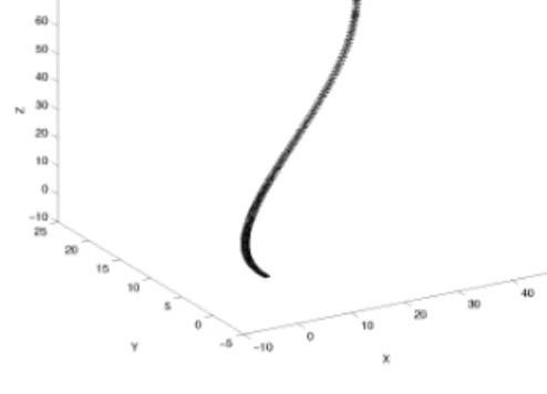
7O 60 50 4O N 30 2O 10 0 -10 . 25 2O % a % Y

(

~ ~ - ~ 50 40 ao o lo -5 _ x

F i g u r e 3: Feedback linearization path.

Once the inputs are obtained, one can use E q u a t i o n 3 to find the forces and set the motor speeds to get the desired lift from each of the rotors.

We can put together these controllers into a hybrid con- troller of the form shown in Figure 4. Hover mode is the central mode, where the model is stabilized by keeping

the positions

(x,y,z)

constant and (0,~,O) angles zero.

The basic commands will be switched from this hover mode. Mode Take-off z=O ~>0 z<z_fly Mode Landing ~<0 z>O . . . . \ .... ~ \z__z~ r~:~-~ / - y=y d

2 \

( x_d, y_d, z_d ~ " ( phi<phi_d / ~ e t a _ d , ~ si_d, p h ~ i ~ (or phi>phi_d~

~ p t i = p h i _ d ~

F i g u r e 4: Hybrid Controller Model.

Climb and descend modes change the z-value, while keep- ing the other values constant. These modes will t e r m i n a t e only when the desired z-value is achieved. L e f t / R i g h t mode is responsible for controlling the y-axis motions. As the model tilts around the x-axis, it will start moving on the y-axis. F o r w a r d / R e v e r s e mode tilts around y-axis by changing the ~ angle. The hover mode will switch to the landing mode when the flight is complete.

3.2 B a c k s t e p p i n g C o n t r o l l e r

Backstepping controllers [71 are especially useful when some states are controlled t h r o u g h other states. As it was observed in the previous section, in order to control the x and y motion of the quadrotor, tilt angles need to be controlled. Therefore a backstepping controller has

backstepping with visual servoing have been developed for a traditional helicopter by Hamel and Mahony [8]. The approach here is a bit simpler in implementation, and relies on only very simple estimates of pose.

We will use a small angle assumption on the yaw angle, ¢, to justify neglecting certain terms from Equation 4 to

give 2 -- u 1 sin 0 cos ~ cos ¢ (10)

~) -- - u 1 sin ~ cos ¢.

First we notice that motion in the y-direction can be con- trolled through changes in the roll. This leads to a back- stepping controller for y - ~ control given by

~t3

1

Ul COS ~) COS ¢ ( - 5 y -- 10~) - 9Ul sin ~ cos ¢

--4~t 1 @ COS ~) COS (~ -~- ~t 1 @2 sin ~ cos ¢

+ 2 u 1 ~ sin ~ sin ¢ + u 1 ~ ¢ cos ~ sin ¢

- U l ¢@ cos ~ sin ¢ - U l ~2 sin ~ cos ¢).

(11)

To develop a controller for motion along the x-axis, we

assume the tilt ¢ is slowly varying or cos ¢ ~ c o n s t . This

leads to a backstepping controller for x - 0 of 1

u2 Ul cos 0 cos ~ cos ¢ ( - 5 x - 10:b - 9Ul sin 0 cos ~ cos ¢

- 4 u 1 ~) cos 0 cos ~ cos ¢ + Ul 02 sin 0 cos ~ cos ¢ + 2 u 1 ¢ sin 0 cos ~ sin ¢ + Ul~)¢ cos 0 cos ~ sin ¢

- u i ¢~) cos 0 cos ~ sin ¢ - u i ~2 sin 0 cos ~ cos ¢). (12)

The altitude and the yaw on the other hand, can be con- trolled by a P D controller. Ul g -Jr- .[~pl(Zd -- Z) -Jr- .[~dl(7]d -- Z)

(13)

cos 0 cos -

¢) +

-

b)

i

/\

0 20 40 40 0 2 0 40 time (s) t i m e (s)

teta vs time phi vs time

Y vs time ~° i 15 ,// lO ! \ \ \ i= 0 -5 -10 0 2o time (s) psi v s time 15 ,~ 5 \ 0 -5 -10 4O 0 2O time (s)

o i

-0.5 -1 o 20 40 o 2 0 40 time (s) t i m e (s)

F i g u r e 5: Backstepping controller simulation results. The simulation results in Figures 5 and 6 show the motion of the quadrotor from position (40, 20, 60) to origin. The

70 60 50 40 N 30 20 10 0 -10 . 25 20 % ,5 Y 3 3 J ' ' ~ ~ ~ " 50 40 0 10 -5 _ x

F i g u r e 6: Backstepping controller path.

controller is strong enough to handle random errors which simulate the pose estimation errors and disturbances as shown in Figure 7. The error introduced on x and y has variance of 0.5 cm and error on z has variance of 2 era. The yaw variance is 1.5 degrees. The helicopter moves from 100 cm to 150 cm while reducing the yaw angle from 30 degrees to zero. The mean and standard deviation are found to be 150 cm and 1.7 cm for z and 2.4 degrees and 10.1 degrees for ¢ respectively.

x vs time Y vs time z vs time

E 50 ~ E 50 ~ 200 o lO 20 time (s) teta vs time -5 0 t 1_ 0 2 0 Ime (s) 10 20 time (s) psi vs time o t!o 20 tme (s) phi vs time

~o "I, ,,, ~,~i',,~,?, , '

~5 - 5 0 ~ / 0 t!0 20 0 t!0 20 tme (s) tme (s)

F i g u r e 7: Backstepping controller simulation with random noise at x, y, z and yaw values.

M o v i n g t o a n a r b i t r a r y h e a d i n g

A backstepping controller is used in the previous section to perform tilts around the x and y axes of the helicopter, assuming the desired yaw angle is zero. Using the invari- ances of the system, it is straightforward to see that the same controller can be applied for an arbitrary ~d. The x t and yt axes shown in Figure 8 are

x' = x cos Cd + Y sin Cd

y' = - - x s i n Cd + y COS Cd. (14)

The equation of motion relative to the initial frame can be rotated to align the body frame to the desired yaw angle.

x

y .

A

F4 F 1

Figure

8: Moving along a r b i t r a r y direction to goal. ~~iii~i!i~iiiiiiiiiiiiiiiiiiiiiiiiiiiiiiiiiiiiiiiiiiiiiiiiiiiiii~i~iiii~ii~i~!~!!~i~i~!i!!N ~~~2i~iiiiiiiiiiiiiiiiiiiiiiiiiiiiiiiiiiiiiiiiiiiiiiiiiiiiiiiiiiiiiiiiiiiiiiiiiiiiiiiiii~iiiii~i~ i i i i ii ~ T h e backstepping controller described above will be used

to perform control on the new x t - yt frame and go to the desired point of t h a t frame. Controllers used for yaw and altitude control can also be used in this part. This con- troller can deal with any desired yaw angle. Simulation results are given in Figure 9 for moving to origin with ~d = 60 °.

x vs time Y vs time Z vs time

~°6I! 1 =

0a!,

... 6 t 16( ) 26 6 tim:(s) 26 time (s) lO 5 ~0 -10 _15 l 20 0

v . \ ,

/

G O A L ~ o 2o . . . 2o 2o ti (s) time (s) ti (s)

Figure 9:

Simulation results for backstepping controller with arbitrary heading.

4 Real Time Control and Vision System

To make a helicopter fully autonomous, we need a flight controller as shown in Figure 10. T h e r e is an off-board controller t h a t receives c a m e r a images, processes t h e m and sends control inputs to the on-board processor. The on-board processor stabilizes the model by checking the gyroscopes and listens for the c o m m a n d s sent from the off-board controller. T h e rotor speeds are set accordingly to achieve the desired positions and orientations.

Off-board On-board u . Actuators forces . . Positions

Controller v . Controller I I m ° m e n t s Quadrotor an 'es I I tilts ] Helicopter ]

gl G y r . . . . pes ~ E21g(e s

C a m e r a Environment

Figure

10: Control Diagram.

T h e off-board controller shown in Figure 11 is responsible for the main computation. It processes the images and

sets the goal positions and sends t h e m to the on-board controller via a radio link.

I m a g e s O f f - b o a r d C o n t r o l l e r I m a g e C o m p u - P r o c e s s i n g " t a t i o n R e m o t e B a s i c - C o n t r o l O n - b o a r d C o m m a n d s D e v i c e " C o n t r o l l e r

Figure

11: Off-board controller.

Figure

12: Q u a d r o t o r tracking with a camera. Helicopter pose is e s t i m a t e d by a pose estimation algo- rithm. This algorithm uses 2.5 cm radius colored blobs t h a t are a t t a c h e d to the b o t t o m of the q u a d r o t o r as shown in Figure 12. A blob tracking algorithm is used to get the positions and areas of the blobs on the image plane. T h e n the purpose of the pose estimation algorithm is to obtain

( x , y , z ) positions, pitch angles (0, ~) and the yaw angle (¢) of the helicopter in real-time relative to the c a m e r a frame. T h e position of each blob is calculated as

z~ - ( f x + f y ) ~ / / ( 2 v / A ~ )

• =

Ox) /fx

(16)

Yi = (vi - O y ) z i / f y ,

where f x and f v are the focal lengths in x and y respec-

tively, C is the n u m b e r of pixels per unit area, Ox and

0 v are the image center coordinates, Ai are the area of the blobs and ui and vi are the image coordinates.

¢ - a r c t a n ( y l - y 5 / x l - x 5 )

- arcsin(z4 - z 2 / d )

0 - arcsin(z5 - z l / d ) .

(17)

T h e position of the helicopter is e s t i m a t e d by averaging the five blob positions. A normalization is performed us- ing the real center difference between blobs. Yaw angle can be obtained from blob positions and the tilt angles can be e s t i m a t e d from the height differences of the blobs, where d is given as the distance between blobs in Equa- tion 17. These estimates depend on area calculations, therefore they are sensitive to noise. O t h e r m e t h o d s t h a t do not depend on the area m e a s u r e m e n t s will be imple- m e n t e d to lower the errors in the pitch and roll angle estimation.

5 Q u a d r o t o r E x p e r i m e n t s

The proposed controllers and the pose estimation algo- rithm have been implemented on a remote controlled bat- tery powered helicopter shown in Figure 13a. It is a com- mercially available hobby helicopter called HMX-4. It is about 0.7 kg, 76 cm long between rotor tips and has about 3 minutes flight time. This helicopter has three gyros on board to stabilize the helicopter. There is a R / C receiver and colored blobs at the bottom. The commands can be sent from a PC to the helicopter by a remote control device t h a t uses the parallel port of a PC.

~ ~ t ~ ` ~ : ~ % ` ~ ` ~ ~ . ~ ` ~ ` . . ~ ` . ` ~ ` ` . . .

ii!!!!i

F i g u r e 13: a) Quadrotor Helicopter, b) Experimental Setup.

An experimental setup shown in Figure 13b was prepared to prevent the helicopter from moving too much in the x-y plane, but letting it be able to turn and ascend/descend. Controllers given in Equations 11, 12 and 13 are imple- mented on the experiment. Figure 14 shows results of this experiment, where height, x ,y and yaw angles are being controlled. The mean and standard deviation are found to be 144 cm and 4.26 cm for z and - 1 0 . 2 de- grees and 11.7 degrees for ¢ respectively. The results from the plots show t h a t the proposed controllers con- trol the helicopter's yaw and height well despite the pose estimation errors and the errors introduced by the teth- ering system.This also agrees with the simulation given in Figure 7 where random noise was introduced.

X vs time 50

~'i ',,' lJ ,~J ~i,~, 7'~- ~'-~ ~"~r'~ ~i~

>-

- 5 O '

0 10 20 30 0

time (seconds)

10 20 30 0 10 20 30

time (seconds) time (seconds)

pitch angle-2 vs time yaw angle vs time

0 10 20 30 0 10 20 30 0 10 20 30

time (seconds) time (seconds) time (seconds)

F i g u r e 14: The results of the height x, y and yaw control

experiment.

6 C o n c l u s i o n s a n d F u t u r e W o r k

We have presented a model of a quadrotor helicopter, and introduced several control methods. Simulations of feedback ]inearization and backstepping controllers were implemented and compared using Matlab Simulink. As it can be seen from the simulations the backstepping con- troller works better than the feedback stabilization. The height and yaw control experiment result shown in Sec- tion 5 prove the control system and the vision system's ability to perform the tasks. A helicopter can not be fully autonomous if it depends on an external camera. There- fore our next goal is to use a combination of two cameras; one on-board the helicopter and an other on the ground. This will help to decrease the errors in estimated tilt an- gles as will the use of other pose estimation algorithms t h a t do not depend on area estimates. Our future inter- est will be to use this helicopter for ground-air coopera- tion tasks. Quadrotors' superior maneuverability makes it a good candidate for inspection, chase and other tasks. Another basic advantage of using such a helicopter is the increased payload, therefore cooperative manipulation of objects with flying robots can also be an interesting and challenging research direction.

7 A c k n o w l e d g e m e n t s

We would like to t h a n k John Spletzer for his help for the blob tracking algorithm. We also gratefully acknowledge support from NSF grant NSF-IIS-9876301 and DARPA ITO Grant 130-1303-4-534328-xxxx-2000-0000.

R e f e r e n c e s

[11 A. Gessow, G. Myers,

Aerodynamics of the heli-

copter,

Frederick Ungar Publishing Co, New York, third edition, 1967.

[21 I. Kroo, F. Printz,

Mesicopter Project,

Stanford

University, h t t p : / / a e r o . s t a n f o r d . e d u / m e s i c o p t e r .

[31 J. Borenstein,

Hoverbot Project,

University of

Michigan,

www-personal.engin.umich.edu/~j ohannb/hoverbot.htm.

[41 Hauser, Sastry, Meyer,

Nonlinear control design

for slightly non-minimum phase systems: application to

V/STOL Aircraft,

Automatica, vol 28, No:4, pp 665-679, 1992.

[51 Martin, Devasia, Paden,

A different look at output

tracking: Control of a VTOL aircraft,

Automatica, vo] 32, No:l, pp 101-107, 1996.

[61 T . J . Koo, F. Hoffmann, B.Sinopoli, S. Sastry,

Hy-

brid Control of An Autonomous Helicopter, Proceedings

of IFAC Workshop on Motion Control, Grenoble, France, September 1998.

[71 S. Sastry,

Nonlinear Systems; Analysis, Stability

and Control,

Springer-Verlag, 1999.

[81 T. Hame], R. Mahony,

Visual servoing of a class of

under-actuated dynamic rigid-body systems,

Proceedings of the 39th I E E E Conference on Decision and Control, 2000.