Volatility and correlations for stock markets in the emerging economies
of Central and Eastern Europe: Implications for European investors
By
D. E. Allen, A. Golab and R. Powell
School of Accounting, Finance and Economics, Edith Cowan University
School of Accounting, Finance and Economics & FEMARC Working Paper Series Edith Cowan University
June 2010 Working Paper 1001
Correspondence author: David E. Allen
School of Accounting, Finance and Economics Faculty of Business and Law
Edith Cowan University Joondalup, WA 6027 Australia
Phone: +618 6304 5471 Fax: +618 6304 5271 Email: d.allen@ecu.edu.au
ABSTRACT
This paper examines the European investment implications of the recent European Union (EU) expansion to encompass former Eastern bloc economies. What are the risk and return characteristics of these markets pre- and post-EU? What are the implications for investors within the Euro zone? Should investors diversify outside the Central and Eastern Europe (CEE)? The former Eastern bloc economies constitute emerging markets which typically offer attractive risk-adjusted returns for international investors. In this paper, we explore a number of aspects of this important issue and their implications for CEE based investors, culminating in a Markowitz efficient frontier analysis of these markets pre- and post-EU expansion.
1
1. Introduction
This paper examines the implications for European investors of the recent European Union (EU) expansion to encompass former Eastern bloc economies. Cappiello et al (2006) question whether the formation of European Monetary Union (EMU) within the EU has increased the correlation of national assets? This clearly has important implications for investors wishing to diversify across national markets. What are the implications for growing asset correlations, if they are displayed? Should investors diversify outside the Central and Eastern European (CEE) countries? It could be argued that the former Eastern bloc economies constitute emerging markets which typically offer attractive risk adjusted returns for international investors. In this paper, we explore a number of aspects of this important issue and their implications for CEE based investors culminating in a Markowitz efficient frontier analysis of these markets pre- and post- EU expansion.
On 1st May 2004 the EU welcomed ten and on 1st January 2007 a further two more countries as part of its largest enlargement ever. The countries concerned are: Bulgaria, Czech Republic, Cyprus, Estonia, Hungry, Latvia, Lithuania, Malta, Poland, Romania, Slovakia and Slovenia. In this paper we investigate the interactions between the CEE bloc countries and apply time-series analysis to examine the relationship between stock market index return volatility. This includes a discussion of the volatility process of stock market indices as well as their correlations for the purpose of modelling volatility in these markets and assessing the implications for investors.
The analysis of the relationship between twelve emerging CEE stock markets will be assessed by examination of the individual pair-wise correlation coefficients to test the temporal stability of the co-movements between returns. The investigation of the determinants of cross-country financial interdependence has been studied in a large empirical literature aiming at identifying the role of a set of factors of influence, such as trade intensity (Forbes & Chinn, 2004) financial development (Dellas & Hess, 2005) and business cycle synchronization (Walti, 2005). All of these papers concentrate on similar topics; however their results and conclusions are slightly different. These concerns might be partly explained by the nature of the econometric approaches (cross-section vs. time-series), the measurement of market co-movement and by the nature and the measurement of explanatory factors. Volatility modelling has been one of the most active and successful
2
areas of research in time series econometrics and economic forecasting in recent decades. The modelling of the risk-expected return relationship is of central importance in modern financial theory and of key practical importance to investors. Risk is typically
characterised by uncertainty and measures such as the variance or volatility of a time series. Since 1982 when Engle introduced the Autoregressive Conditional
Heteroskedasticity (ARCH) model the model has been effectively applied to numerous economic and financial datasets in the modelling of financial time series. The original ARCH model generated a huge family of direct descendants. This includes Bollerslev’s (1986) model of generalised ARCH (GARCH), which is currently the most popular and successful time series model. This paper examines a GARCH (1,1) volatility model for the pre- and post-EU period in the context of the previously mentioned economies with a view to analysing the impact of EU membership on the behaviour of financial assets in these economies.
During the past few years a few empirical studies have been undertaken on four of the twelve mentioned CEE emerging markets: the Czech Republic, Hungry, Poland and Slovakia. These papers mainly examine correlations in stock returns and their volatility in the Polish and Slovakian stock markets (Hranaiova, 1999), time varying co-movements while applying Engle’s (2002) GARCH models between developed economies such as France, Germany and the UK and emerging ones; Czech Republic, Hungry and Poland (Scheicher, 2001) then (Egert & Kocenda, 2007)). Worthington & Higgs (2004) analysed market efficiency using methods applying the serial correlation coefficient, ADF
(Augmented Dickey-Fuller), PP (Phillips-Perron) and KPSS (Kwiatkowski, Phillips, Schmidt and Shin) unit root tests and MVR (multiple variance ration) tests. Another paper constructed on a random walk framework is the paper by Cuaresma and Hlouskova (2005). An alternative issue to market efficiency is based on the degree of financial integration amongst the stock exchange markets in the Czech Republic, Hungry, Poland and Slovakia in comparison with the euro zone market (Babetskii, Komarek, &
Komarkova, 2007). The EMU equity market’s volatility and correlation vs. US ones is also the subject of a paper written by Kearney & Poti (2008) and for global markets that of Capiello et al (2006). Another approach, adopted by Bruggemann and Trenkler (2007) discusses the catching up process in the Czech Republic, Hungry and Poland by
investigating GDP behaviour. The spillover effects of emerging markets had been
3
european countries have been discussed. Overall, the majority of past studies of stock markets correlation and volatility have been undertaken on developed markets or advanced emerging markets such as the Czech Republic, Hungary and Poland whilst the behaviour and inter-relationship of all others has been neglected. Our paper seeks to fill this empirical void.
Jorion and Goetzemann (1999) suggested that many emerging markets are actually re-emerging markets, that for various reasons, have gone through a period of relative decline. They pointed out that Poland, Romania and Czechoslovakia had active equity markets in the 1920s prior to being subsumed in the Eastern bloc. This means that their attractive returns apparently offered by emerging markets may be a temporary phenomenon, an observation they backed up by simulations.
This paper is structured as follows. Section 2 presents descriptive statistics and unconditional volatility metrics and section 3 introduces the methodology applied to evaluate stock market relationships (this includes unit root tests, pairwise correlations and a GARCH (1,1) volatility model), followed by a Markowitz efficient frontier analysis pre- and post-enlargement. In section 4 we discuss the results from the calculations and section 5 summarises the findings.
2. Data and Summary Statistics
The statistical data in this study consists of the daily stock market indices in the twelve CEE stock markets1 (Bulgaria, Czech Republic, Cyprus, Estonia, Hungry, Latvia, Lithuania, Malta, Poland, Romania, Slovakia and Slovenia). The data is obtained from DataStream and SIRCA’s databases for the period from January 1, 1995 to September 30, 2009. The twelve countries joined the EU during the latest two enlargements which took place on 1st May 2004 for the Czech Republic, Cyprus, Estonia, Hungry, Latvia, Lithuania, Malta, Poland, Slovakia and Slovenia and 1st January 2007 for Bulgaria and Romania. Based on those two accession dates the sample period is divided into two phases: pre-EU period (1st Jan 1995 -30th Apr 2004 for the first enlargement and 1st Jan 1995 - 31st Dec 2006 for the second one) and post-EU (1st May 2004 - 30th Sep 2009 for the first
1
SOFIX (Bulgaria), SEPX (Czech Republic), CYSE (Cyprus), OMX Tallinn Stock Exchange (Estonia), BUX
(Hungry), OMX Riga Stock Exchange (Latvia), OMX Vilnius Stock Exchange (Lithuania), MSE (Malta), WIG (Poland), BET (Romania), SAX (Slovakia) and SBI (Slovenia)
4
enlargement and 1st Jan 2007 - 30th Sep 2009 for the second one). The analysis is based in terms of one common currency in which stock market prices are expressed: the euro, whose conversion from local currencies gives basically the same findings (Syriopoulos, 2007).
3. Empirical Methodology
This paper uses several methods to test the behaviour of the return series of the twelve CEE markets. Firstly the hypothesis of unit roots occurrence in the series is tested; then the correlation coefficients are analysed. The applied methodology is analysed for two
specified periods: the pre-EU and post-EU phases as explained previously.
3.1 Non-stationarity of time series
There are a number of tests for non-stationarity of time series data. This paper adopts two of them: the Augmented Dickey-Fuller (ADF) test (Dickey & Fuller, 1981) and Phillips-Perron (PP) non-parametric test (Phillips & Phillips-Perron, 1988). If a series is defined as stationary the mean and auto-covariance of the data series do not depend on time.
The results are shown in Table 2. The fact that the levels price series are non-stationary is consistent with market efficiency and a reasonable level of competition in these markets. For example, if prices were trending and predictable this would have strong implications for market efficiency and be evidence of a lack of competitiveness.
3.2 Pairwise correlation
Correlation is a measure of co-movements between two returns series. Strong positive correlation indicates that upward movements in one returns series tend to be accompanied by upward movements in the other and similarly downward movements of the two series tend to go together (Engle, 2002) and vice-versa for negative correlation. The pairwise correlation of the selected 12 European emerging markets is computed as below:
, =,
5
where the covariance between two variables x and y is defined as the expected value of the product − − and given as:
, = − − . (2)
3.3 Volatility measure
Pegan and Schwert (1990) provide systematic comparisons of volatility models developed in the literature. The GARCH class of models has proven to be particularly suited for modelling the behaviour of financial time series. These models are capable of capturing the three most common empirical observations in daily return data such as: fat tails due to time-varying volatility, skewness resulting from mean non-stationarity, and volatility clustering.
GARCH models can provide a parsimonious parameterization of a high-order ARCH process. Moreover, the model performs much better than the ARCH model due to its containing more sensible constrains on coefficients and using only a few parameters (Ling & McAleer, 2002). GARCH (1,1) model is equivalent to an infinite ARCH model with exponentially declining weight and takes the form of
=ωωωω+ ∑ ααααεεεε + ∑! ββββ, (3) where for the GARCH process to exist, ω> 0, α and β ≥ 0 are sufficient conditions for the conditional variances to be positive. The conditional variance depends on constant value of
ω, the error/reaction coefficient α and lag/persistence coefficient β. ε"#$ is the ARCH term and represents news about volatility from the previous period and ℎ"# the GARCH term, which is the last period’s forecast variance. Both parameters (α and β) are sensitive to the historic data used for the model. The size of the parameters α and β determine the short run dynamic of the resulting volatility time series. A large GARCH lag coefficient β indicates that shocks to conditional variance take a long time to die out, so volatility is “persistent”. Large ARCH error coefficients α mean that volatility reacts quite intensively to market movements and so if α is relatively high and β is relatively low then volatility tends to be more “spiky”. In practice, numerous studies have demonstrated that a GARCH (1,1) specification is often most appropriate. The coefficients of the model are easily interpreted,
6
with the estimate of α1 showing the impact of current news on the conditional variance
process and the estimate of β1 the persistence of volatility to a shock or, alternatively, the
impact of ‘old’ news on volatility. The necessary and sufficient conditions for the second moment to exist for the GARCH (1,1) process is given by the definition that coefficients of
α and β need to be summed to less than unity in each case.
3.4 Markowitz efficient frontiers
To ascertain the optimal portfolio mix of the 12 countries, we calculate the Markowitz (1952) efficient frontier pre- and post-EU expansion. This frontier represents the combination of assets which give the lowest risk as measured by volatility (standard deviation) for any selected level of return and is obtained by minimising
&∑ '( + ∑ ∑ '( () ')*) (4)
where: σp is the portfolio standard deviation, wi - the weights of the individual assets in the
portfolio, +,$ -the variance of rates of return for asset I and Covij - the covariance between
the asset returns (R) in the portfolio.
This optimisation is repeated for various levels of R to minimise σ (or various levels of σ
to maximise R). Using matrix multiplication, we calculate a variance-covariance matrix from the correlations shown in Table 2 and Table 3 and the standard deviations in Table 1. The two endpoints of the frontier are the maximum mean return as per Table 1 and its associated return, and the minimum portfolio risk and its associated return obtained from the above optimization function.
4. Empirical Results 4.1 Descriptive statistics
Table 1 presents descriptive statistics for the daily returns for the periods pre- and post-EU. Daily returns are defined as logarithmic price relatives: -"= ./0"/0"# × 100. In every case the return series has a mean value close to zero and a distribution characterized by non-normality (Jarque-Bera statistics). The highest mean of returns in pre-EU period can
7
Table 1: Stock market descriptive statistics
Mean Median Max Min St Dev Skew Kurtos Jarque-Bera Normality p-value Obs Pre-EU period Bulgaria 0.155 0.044 21.073 -20.899 1.857 -0.447 38.678 85710.45 0.000 1615 Czech Rep 0.005 0.000 5.819 -7.077 1.187 -0.154 5.225 527.48 0.000 2509 Cyprus N/A N/A N/A N/A N/A N/A N/A N/A N/A N/A Estonia 0.077 0.076 7.352 -5.874 1.102 -0.086 6.969 742.47 0.000 1129 Hungary 0.081 0.025 13.616 -18.034 1.789 -0.847 16.502 16.50 0.000 2692 Latvia 0.103 0.039 9.461 -14.705 1.831 -1.249 20.157 14141.68 0.000 1129 Lithuania 0.070 0.038 4.580 -10.216 0.889 -1.168 20.895 15321.54 0.000 1129 Malta 0.057 0.000 9.573 -7.589 0.920 2.244 26.658 37570.67 0.000 1555 Poland 0.037 0.000 7.893 -10.286 1.710 -0.077 6.053 973.45 0.000 2499 Romania 0.086 0.000 11.544 -11.901 1.717 -0.012 9.731 4568.78 0.000 2420 Slovakia 0.018 0.000 27.554 -12.452 1.734 2.185 40.294 161795.5 0.000 2754 Slovenia 0.048 0.000 11.012 -11.344 1.255 -0.306 15.629 17951.95 0.000 2695 Post-EU period Bulgaria - 0.128 0.000 7.292 -11.359 1.911 -0.832 8.154 887.682 0.000 726 Czech Rep 0.026 0.056 12.264 -16.185 1.762 -0.593 16.897 11518.66 0.000 1396 Cyprus 0.053 0.000 12.124 -10.881 2.203 0.001 7.302 1026.47 0.000 1331 Estonia 0.015 0.023 12.094 -7.045 1.192 0.196 16.261 10238.40 0.000 1396 Hungary 0.043 0.028 13.177 -12.649 1.816 -0.184 9.927 2849.37 0.000 1396 Latvia - 0.004 0.000 9.156 -7.414 1.331 0.011 9.329 2330.35 0.000 1396 Lithuania 0.021 0.005 11.001 -9.111 1.301 0.123 17.468 12180.26 0.000 1396 Malta 0.013 0.000 4.736 -4.536 0.813 0.067 8.937 2088.20 0.000 1396 Poland 0.032 0.017 6.083 -8.288 1.433 -0.429 6.236 664.05 0.000 1396 Romania - 0.083 0.000 10.091 -13.117 2.328 -0.492 6.604 422.33 0.000 726 Slovakia 0.032 0.014 11.880 -9.577 1.105 0.111 20.206 17532.81 0.000 1396 Slovenia - 0.003 0.001 7.681 -8.299 1.147 -0.771 13.842 7101.94 0.000 1396
be observed in Bulgaria (0.086) and Romania (0.155) stock markets, countries which joined the EU at the latest expansion. Those two countries, however, have the lowest and negative return in the post-EU period of -0.083 for Romania and -0.128 for Bulgaria. Next to those countries there are other two which as well have negative. There are Slovenia (-0.003), Latvia (-0.004). The highest mean return is assigned to Cyprus (0.053). If the data is normally distributed, then the mean and variance would completely describe the
distribution of the data and the higher movements of skewness and kurtosis would provide no additional information about that distribution. However, the data contains positive skewness for two markets for the pre-EU period and on six occasions in the post-EU period. The skewness is greater than zero in all cases but one, post-EU Cyprus, where skewness is very close to zero (0.001). All other values for skewness are negative which implies that the distribution has a long left tail, whereas the relevant Jarque-Bera statistics
8
indicate rejection of the normality hypothesis. All markets generate kurtosis statistics more than 3 (which is the benchmark for a normal distribution) which indicates the series is characterised by leptokurtosis. This means that the distribution of the data contains a greater number of observations in the tails than that found in a normal distribution. Whilst it is possible to individually test the significance of the skewness and kurtosis, the more common approach is the joint test based on the calculation of the Jarque-Bera statistics and comparison to its critical values, which is shown in Table 1.
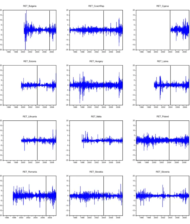
Figure 1: Return series of daily returns
-20 -15 -10 -5 0 5 10 15 20 1996 1998 2000 2002 2004 2006 2008 RET_Bulgaria -20 -15 -10 -5 0 5 10 15 20 1996 1998 2000 2002 2004 2006 2008 RET_CzechRep -20 -15 -10 -5 0 5 10 15 20 1996 1998 2000 2002 2004 2006 2008 RET_Cyprus -20 -15 -10 -5 0 5 10 15 20 1996 1998 2000 2002 2004 2006 2008 RET_Estonia -20 -15 -10 -5 0 5 10 15 20 1996 1998 2000 2002 2004 2006 2008 RET_Hungary -20 -15 -10 -5 0 5 10 15 20 1996 1998 2000 2002 2004 2006 2008 RET_Latvia -20 -15 -10 -5 0 5 10 15 20 1996 1998 2000 2002 2004 2006 2008 RET_Lithuania -20 -15 -10 -5 0 5 10 15 20 1996 1998 2000 2002 2004 2006 2008 RET_Malta -20 -15 -10 -5 0 5 10 15 20 1996 1998 2000 2002 2004 2006 2008 RET_Poland -20 -15 -10 -5 0 5 10 15 20 1996 1998 2000 2002 2004 2006 2008 RET_Romania -20 -15 -10 -5 0 5 10 15 20 1996 1998 2000 2002 2004 2006 2008 RET_Slovakia -20 -15 -10 -5 0 5 10 15 20 1996 1998 2000 2002 2004 2006 2008 RET_Slovenia
9
Volatility measured by the standard deviation of daily returns shows that again Bulgaria’s stock market is the most volatile one in both examined periods. The least risk lowest volatility market is Malta’s stock market. The volatility of CEE countries can be observed on Figure 1 that provides plots of daily returns for all twelve countries. Every graph has been divided by a vertical line into two parts showing pre- and post-EU phases. Figure 1 of the return series clearly shows volatility clustering, which explains large (small) changes tend to be followed by large (small) changes of either signs. The volatility clustering absorbs as well good (positive variation) and bad (negative oscillation) information news. This graph shows also that there are massive fluctuations during certain periods, such as the 1998 Russian crisis, the late 1990s/early 2000s internet “bubble”, the 9/11 terrorist attacks on World Trade Centre, the 2007 global financial market turmoil, and the 2009 world financial downturn.
4.2 Non-stationarity of the levels prices time series
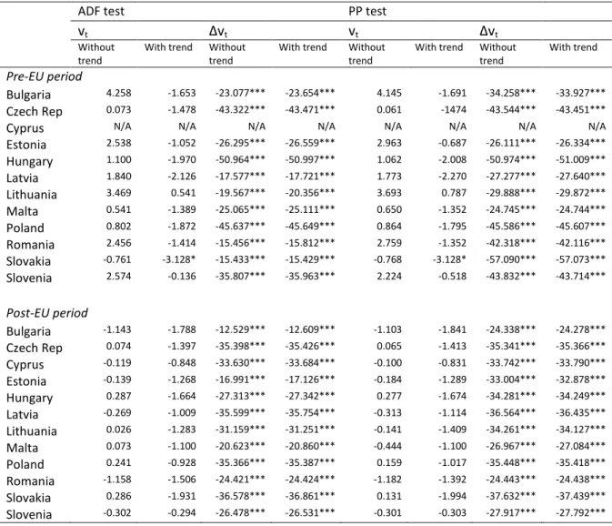
In order to test for the presence of stochastic non-stationarity in the return series data; two unit root tests: the ADF and the PP tests have been applied. Table 2 presents results from both tests. The customary finding, consistent with work on market efficiency is that price levels series should contain a unit root; suggesting a lack of predictability. If there is a rejection of unit roots in the price levels series this may be consistent with the existence of price trends and the ability to predict prices. However, in only one case; that of Slovakia in the pre-EU period, do we reject the unit root in the price levels series when we add a trend to the model. This result is consistent for both the ADF and the PP tests. However, it vanishes in the post-EU period. The evidence for the price levels series is consistent with the existence of competitive markets.
For the returns, or differenced series, we find evidence strongly suggesting the existence of stationarity. Each of the test scores are below the critical value at the 5% level and this result is not sensitive to the presence of an intercept term and trend. Both tests were
performed using the maximum lag length in each case. The ADF and PP test statistic value has a probability value of 0.01 for all markets, providing evidence that we may reject the null hypothesis of existence of the unit roots for return series. Hence, the ADF and PP tests clearly indicate that the return data is stationary. We may conclude that if the price index
10
series had not rejected the hypothesis of unit root existence then the stock markets price series could display trend behaviour. However, our results suggest the contrary.
Table 2: Unit root tests on price levels and first differences
ADF test PP test
vt Δvt vt Δvt
Without trend
With trend Without trend
With trend Without trend
With trend Without trend
With trend
Pre-EU period
Bulgaria 4.258 -1.653 -23.077*** -23.654*** 4.145 -1.691 -34.258*** -33.927*** Czech Rep 0.073 -1.478 -43.322*** -43.471*** 0.061 -1474 -43.544*** -43.451***
Cyprus N/A N/A N/A N/A N/A N/A N/A N/A
Estonia 2.538 -1.052 -26.295*** -26.559*** 2.963 -0.687 -26.111*** -26.334*** Hungary 1.100 -1.970 -50.964*** -50.997*** 1.062 -2.008 -50.974*** -51.009*** Latvia 1.840 -2.126 -17.577*** -17.721*** 1.773 -2.270 -27.277*** -27.640*** Lithuania 3.469 0.541 -19.567*** -20.356*** 3.693 0.787 -29.888*** -29.872*** Malta 0.541 -1.389 -25.065*** -25.111*** 0.650 -1.352 -24.745*** -24.744*** Poland 0.802 -1.872 -45.637*** -45.649*** 0.864 -1.795 -45.586*** -45.607*** Romania 2.456 -1.414 -15.456*** -15.812*** 2.759 -1.352 -42.318*** -42.116*** Slovakia -0.761 -3.128* -15.433*** -15.429*** -0.768 -3.128* -57.090*** -57.073*** Slovenia 2.574 -0.136 -35.807*** -35.963*** 2.224 -0.518 -43.832*** -43.714*** Post-EU period Bulgaria -1.143 -1.788 -12.529*** -12.609*** -1.103 -1.841 -24.338*** -24.278*** Czech Rep 0.074 -1.397 -35.398*** -35.426*** 0.065 -1.413 -35.341*** -35.366*** Cyprus -0.119 -0.848 -33.630*** -33.684*** -0.100 -0.831 -33.742*** -33.790*** Estonia -0.139 -1.268 -16.991*** -17.126*** -0.184 -1.289 -33.004*** -32.878*** Hungary 0.287 -1.664 -27.313*** -27.342*** 0.277 -1.674 -34.281*** -34.249*** Latvia -0.269 -1.009 -35.599*** -35.754*** -0.313 -1.114 -36.564*** -36.435*** Lithuania 0.026 -1.283 -31.159*** -31.251*** -0.141 -1.409 -34.261*** -34.127*** Malta 0.073 -1.100 -20.623*** -20.860*** -0.444 -1.100 -26.967*** -27.084*** Poland 0.241 -0.928 -35.366*** -35.387*** 0.159 -1.017 -35.448*** -35.418*** Romania -1.158 -1.506 -24.421*** -24.424*** -1.182 -1.392 -24.443*** -24.438*** Slovakia 0.286 -1.931 -36.578*** -36.861*** 0.131 -1.994 -37.632*** -37.439*** Slovenia -0.302 -0.294 -26.478*** -26.531*** -0.301 -0.303 -27.917*** -27.792*** vt: variable in levels; ∆vt: variable in first difference
Critical values/without trend: -2.566 at the 1% level; -1.941 at the 5% level; -1.617 at 10% level Critical values/with trend: -3.962 at the 1% level; -3.412 at the 5% level; -3.128 at 10% level MacKinnon (1996) one-sided p-value
Significance levels: *** 0 .01% , ** 0.05%, * 0.10
4.3 Pairwise correlation
The prior expectation of this analysis, based on previous research, is one of weak expected comovements between the countries studied (Scheicher, 2001; Syriopoulos, 2007);
however some of the cross country correlations may be found to be significant. In our data the pre-EU period shows correlations on most occasions to be weak and the correlation coefficients do not exceed a value of 0.1 (Table 3). It is observable that Slovakia’s stock market remains isolated from all others; it demonstrates negative correlation with most of
11
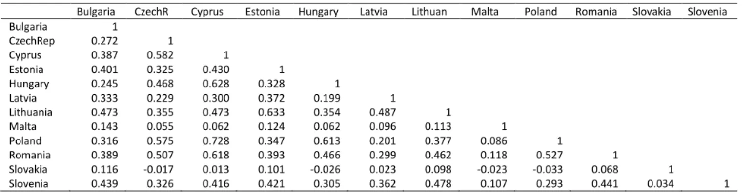
the other countries except Latvia, Malta and Poland, where the value of the correlation coefficient is positive but still very small: 0.014, 0.010 and 0.032 respectively. The other market showing negative correlation is Bulgaria. This market is inversely correlated with Poland, Romania and Slovakia and is very lowly correlated with all other CEE countries. On the other hand, the markets of the Czech Republic, Hungary and Poland are reasonably highly correlated with each other, showing average correlations of 0.452. Estonia’s stock market is different from all the other weakly correlated markets with average correlation of 0.233 to Hungary, Lithuania and Poland. The post-EU period shows some changes with an increase of stock markets inter-relations which end up with stronger correlations between countries. As such we can see that the values of the correlation coefficients significantly increased after all the countries concerned joined the EU. Table 4 and Table 5 demonstrate those correlation coefficients and as previously we can see a very strong relationship between three countries: the Czech Republic, Hungary and Poland, however the stock markets of Romania and Cyprus should be emphasized here as well. (Cyprus has not been mentioned in the pre-EU discussion as data for this market is only available for the post-EU phase) Yet again we can see that the stock market of Slovakia is different to all others with the addition of Malta’s stock market. Both of them show very weak correlations to all the other countries. A striking fact is that after the last EU accession by Bulgaria and Romania on 1st January 2007 the correlation coefficient between these two is stronger than had been the case before they became members of the EU, which is shown in Table 5.
Overall, the correlation coefficients between the CEE stock markets are found to be
relatively low and on some occasions negative in the pre-EU period. In the post-EU period the correlation coefficients between the CEE markets are higher which indicates they strengthened. This period also demonstrates that pre-EU negative correlations turn to being positive ones in the post-EU period. The stock markets of the Czech Republic, Hungary and Poland indicate high and positive pairwise correlation, whereas the smaller markets of Malta and Slovakia remain still isolated compared to their peers.
The increase in the correlations in the post-EU period means that the scope for investors diversifying into these new markets, investing in Euros has been diminished. Capiello et al (2006) find much higher correlations amongst bond indices across EU members’ states than is the case with equity indices. This is perhaps not surprising given the influence of common monetary policies. Jorion and Goetzemann (1999) undertake simulations of the
12
characteristics of emerging markets and suggest that high returns and low covariances with developed markets are characteristics of ‘emergence’, but not necessarily long-term
characteristics. They also point out that many today’s emerging markets are: ‘re-emerging’ markets that had previously been prominent but had, for various reasons sunk from the sight of international investors. They include Poland, Romania and Czechoslovakia in this category noting that they had active equity markets in the 1920s.
Table 3: Correlation coefficient matrix for pre-EU period, 1995-2004
Bulgaria CzechR Estonia Hungary Latvia Lithuan Malta Poland Romania Slovakia Slovenia Bulgaria 1 CzechRep 0.035 1 Estonia 0.094 0.277 1 Hungary 0.044 0.474 0.251 1 Latvia 0.021 0.043 0.074 -0.007 1 Lithuania 0.030 0.075 0.229 0.057 0.039 1 Malta 0.050 0.014 0.020 0.060 0.001 0.003 1 Poland -0.042 0.425 0.219 0.456 -0.002 0.072 0.021 1 Romania -0.037 0.074 0.036 0.083 0.036 0.035 0.034 0.043 1 Slovakia -0.009 -0.026 -0.054 -0.028 0.014 -0.033 0.010 0.032 -0.028 1 Slovenia 0.012 0.059 0.065 0.080 0.019 -0.039 0.008 0.007 0.066 0.047 1
Table 4: Correlation coefficient matrix for post-EU period, 2004-2009
Bulgaria CzechR Cyprus Estonia Hungary Latvia Lithuan Malta Poland Romania Slovakia Slovenia Bulgaria 1 CzechRep 0.230 1 Cyprus 0.325 0.511 1 Estonia 0.351 0.289 0.379 1 Hungary 0.187 0.403 0.612 0.285 1 Latvia 0.274 0.207 0.249 0.325 0.175 1 Lithuania 0.394 0.294 0.406 0.549 0.292 0.409 1 Malta 0.097 0.059 0.023 0.074 0.033 0.080 0.087 1 Poland 0.261 0.482 0.685 0.305 0.618 0.177 0.308 0.035 1 Romania 0.319 0.408 0.500 0.328 0.359 0.238 0.363 0.065 0.414 1 Slovakia 0.100 0.016 0.029 0.091 0.009 0.014 0.092 0.008 -0.023 0.046 1 Slovenia 0.380 0.297 0.375 0.379 0.255 0.301 0.414 0.061 0.265 0.376 0.027 1
Table 5: Correlation coefficient matrix for post-EU period, 2004-2007
Bulgaria CzechR Cyprus Estonia Hungary Latvia Lithuan Malta Poland Romania Slovakia Slovenia Bulgaria 1 CzechRep 0.272 1 Cyprus 0.387 0.582 1 Estonia 0.401 0.325 0.430 1 Hungary 0.245 0.468 0.628 0.328 1 Latvia 0.333 0.229 0.300 0.372 0.199 1 Lithuania 0.473 0.355 0.473 0.633 0.354 0.487 1 Malta 0.143 0.055 0.062 0.124 0.062 0.096 0.113 1 Poland 0.316 0.575 0.728 0.347 0.613 0.201 0.377 0.086 1 Romania 0.389 0.507 0.618 0.393 0.466 0.299 0.462 0.118 0.527 1 Slovakia 0.116 -0.017 0.013 0.101 -0.026 0.023 0.098 -0.023 -0.033 0.068 1 Slovenia 0.439 0.326 0.416 0.421 0.305 0.362 0.478 0.107 0.293 0.441 0.034 1
13
4.4 Volatility measure
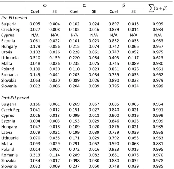
For the GARCH process to be stationary, the parameters in the variance equation must sum to less than one (for GARCH (1,1) model α+β < 1). The closer the sum to one, the less stable the variance will be in the long run, and the more permanent will be changes in the level of volatility as a consequence of “volatility shocks”. Conversely, the smaller is this sum relative to one, the more transient will be the effect of the volatility shocks, and the less of an adjustment there will be to expected returns. To test ARCH and GARCH coefficients values we again run the test for all twelve CEE stock markets in two time periods: pre- and post- EU. Error! Reference source not found. presents details of the GARCH model. The α and β coefficients are positive, significant and summed to less than one for each stock market.
Table 6: Estimated GARCH (1,1) model on return series data
ω α β
56 + 7
Coef SE Coef SE Coef SE
Pre-EU period
Bulgaria 0.005 0.004 0.102 0.024 0.897 0.015 0.999 Czech Rep 0.027 0.008 0.105 0.016 0.879 0.014 0.984 Cyprus N/A N/A N/A N/A N/A N/A N/A Estonia 0.061 0.022 0.101 0.023 0.852 0.035 0.953 Hungary 0.179 0.056 0.215 0.074 0.742 0.066 0.957 Latvia 0.102 0.036 0.228 0.061 0.747 0.052 0.975 Lithuania 0.310 0.159 0.220 0.084 0.403 0.117 0.623 Malta 0.048 0.026 0.235 0.075 0.745 0.089 0.980 Poland 0.109 0.030 0.110 0.023 0.851 0.026 0.961 Romania 0.149 0.041 0.203 0.034 0.759 0.035 0.962 Slovakia 0.063 0.030 0.089 0.026 0.890 0.032 0.979 Slovenia 0.022 0.006 0.204 0.039 0.795 0.034 0.999 Post-EU period Bulgaria 0.166 0.061 0.269 0.067 0.685 0.065 0.954 Czech Rep 0.041 0.012 0.151 0.027 0.840 0.021 0.991 Cyprus 0.026 0.013 0.099 0.018 0.900 0.016 0.999 Estonia 0.004 0.003 0.153 0.029 0.846 0.023 0.999 Hungary 0.047 0.018 0.109 0.020 0.876 0.021 0.985 Latvia 0.079 0.021 0.199 0.039 0.759 0.039 0.958 Lithuania 0.070 0.035 0.171 0.029 0.792 0.053 0.963 Malta 0.093 0.029 0.291 0.052 0.590 0.068 0.881 Poland 0.014 0.007 0.072 0.016 0.923 0.015 0.995 Romania 0.313 0.114 0.289 0.082 0.681 0.073 0.970 Slovakia 0.034 0.017 0.098 0.030 0.880 0.032 0.978 Slovenia 0.032 0.009 0.237 0.050 0.748 0.039 0.985
14
Figure 2: Conditional variance of GARCH (1,1) model
Volatility persistence in the CEE countries is generally very high. Overall, Hungary, Poland, Czech Republic, Romania and Slovakia show similar volatility measure behaviour through the whole testing period with no dramatic changes referring to the accession to EU. The pre-EU period seems to be less volatile in Estonia and Lithuania. On the other hand, the post-EU period is less volatile for Bulgaria, Latvia, Malta and Slovenia. The sum of ARCH and GARCH coefficients (α+β) is very close to one, indicating that volatility
0 20 40 60 80 100 120 01 02 03 04 05 06 07 08 09 Bulgaria 0 10 20 30 40 50 60 70 96 98 00 02 04 06 08 Czech Rep 0 4 8 12 16 20 24 00 01 02 03 04 05 06 07 08 09 Estonia 0 10 20 30 40 50 60 70 94 96 98 00 02 04 06 08 Hungary 0 10 20 30 40 50 60 70 80 90 00 01 02 03 04 05 06 07 08 09 Latvia 0 10 20 30 40 50 00 01 02 03 04 05 06 07 08 09 Lithuania 0 5 10 15 20 25 30 98 99 00 01 02 03 04 05 06 07 08 09 Malta 0 4 8 12 16 20 24 96 98 00 02 04 06 08 Poland 0 10 20 30 40 50 60 98 99 00 01 02 03 04 05 06 07 08 09 Romania 0 20 40 60 80 100 94 96 98 00 02 04 06 08 Slovakia 0 10 20 30 40 50 60 94 96 98 00 02 04 06 08 Slovenia 0 10 20 30 40 50 05 05 06 06 07 07 08 08 09 09 Cyprus
15
shocks are quite persistent, which is often observed in high frequency financial data and is a characteristic for emerging markets. Overall, the dynamics of volatility in the post-EU period seems to be more stable and even for all the stock markets as the standard deviation for this period is 0.032 (for mean α+β = 0.972) with comparison to the pre-EU period where the standard deviation is 3.3 times larger (0.107) with mean equal to 0.943. The conditional variance of the GARCH (1,1) model presented in
16
Figure 2 illustrates that the conditional variance shows a great deal of volatility over the defined period of time with a number of fairly large spikes observable. Those spikes are normally associated with the arrival of major news to the market which has an influence on price adjustment. The last high spike visible in almost all the countries and observed in
17
Figure 2 is at the end of 2008 which is the US subprime mortgage crisis time and world economic turndown. The evidence of volatility evidently justifies the modelling of time varying conditional variances as opposed to the standard assumption of homoscedasticity.
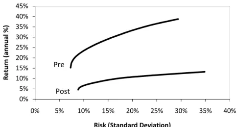
4.5 Markowitz Efficient Frontier Analysis
To calculate the Markowitz efficient frontiers for these markets pre- and post-EU
expansion, as shown in Figure 3 below and summarized in Table 7, we use the correlations shown in Table 3 and Table 4 and the standard deviations in Table 1. The two endpoints of the frontier are the maximum mean return as per Table 1 and its’ associated return, and the minimum portfolio risk and its’ associated return obtained from the above optimization function. Using these highest and lowest return points, we calculate equidistant intervening return points to obtain a total of ten return scenarios. We minimize σ for each of these return scenarios to obtain pre- and post-EU efficient frontiers as shown in the following Figure 3:
The frontier shows a downward shift post-EU incorporation, meaning lower available returns for any given level of risk. Our concern is not so much with the levels of the frontier as these are influenced by global market events such as the Global Financial Crisis in the post-EU period, but rather with the optimal risk-return combination of assets that make up the frontier. These are shown in Table 7.
Figure 3: Efficient Frontier
0% 5% 10% 15% 20% 25% 30% 35% 40% 45% 0% 5% 10% 15% 20% 25% 30% 35% 40% R e tu rn ( a n n u a l % )
Risk (Standard Deviation)
Pre
18
Table 7: Optimal Asset Allocation
Pre-EU period
return 38.8% 36.1% 33.5% 30.9% 28.3% 25.7% 23.1% 20.5% 17.9% 15.3% stdev 29.4% 24.3% 20.3% 17.1% 14.2% 11.7% 9.8% 8.3% 7.5% 7.3%
Optimal portfolio mix for each return level:
Bulgaria 100.0% 80.4% 64.6% 51.4% 40.0% 30.0% 21.4% 14.1% 8.3% 4.8% CzechR 0.0% 0.0% 0.0% 0.0% 0.0% 0.0% 0.0% 0.0% 1.0% 8.6% Estonia 0.0% 0.0% 0.0% 4.5% 8.5% 10.6% 10.9% 10.7% 9.7% 7.6% Hungary 0.0% 0.0% 1.6% 5.5% 5.9% 5.7% 4.9% 4.0% 2.0% 0.0% Latvia 0.0% 18.0% 21.6% 20.5% 17.6% 14.6% 11.7% 8.9% 6.5% 4.8% Lithuania 0.0% 0.0% 0.0% 3.6% 14.2% 20.6% 23.3% 24.5% 24.5% 23.7% Malta 0.0% 0.0% 0.0% 0.0% 0.0% 6.1% 14.0% 19.2% 22.5% 23.6% Poland 0.0% 0.0% 0.0% 0.0% 0.0% 0.0% 0.0% 0.0% 2.3% 2.2% Romania 0.0% 1.5% 12.2% 14.5% 13.8% 12.4% 10.4% 8.4% 6.7% 5.3% Slovakia 0.0% 0.0% 0.0% 0.0% 0.0% 0.0% 0.0% 2.3% 5.7% 7.4% Slovenia 0.0% 0.0% 0.0% 0.0% 0.0% 0.0% 3.6% 7.9% 10.9% 11.9%
Post -EU period
return 13.3% 12.3% 11.3% 10.4% 9.4% 8.4% 7.5% 6.5% 5.6% 4.6% stdev 34.8% 28.6% 22.9% 18.2% 15.2% 13.1% 11.3% 9.9% 9.1% 8.9%
Optimal portfolio mix for each return level:
Bulgaria 0.0% 0.0% 0.0% 0.0% 0.0% 0.0% 0.0% 0.0% 0.0% 0.0% CzechR 0.0% 0.0% 0.0% 0.0% 0.0% 0.0% 0.0% 0.5% 1.3% 1.1% Cyprus 100.0% 76.9% 56.7% 36.4% 19.9% 14.3% 8.6% 2.8% 0.0% 0.0% Estonia 0.0% 0.0% 0.0% 0.0% 0.0% 0.0% 0.0% 1.2% 6.5% 9.1% Hungary 0.0% 9.1% 12.7% 16.4% 18.3% 14.8% 11.3% 7.9% 4.0% 0.3% Latvia 0.0% 0.0% 0.0% 0.0% 0.0% 0.0% 0.0% 0.0% 2.3% 9.7% Lithuania 0.0% 0.0% 0.0% 0.0% 0.0% 0.0% 1.8% 5.4% 4.7% 1.8% Malta 0.0% 0.0% 0.0% 0.0% 3.1% 15.1% 26.0% 34.5% 40.5% 44.0% Poland 0.0% 0.0% 0.0% 0.0% 0.9% 4.8% 8.4% 11.0% 10.9% 9.5% Romania 0.0% 0.0% 0.0% 0.0% 0.0% 0.0% 0.0% 0.0% 0.0% 0.0% Slovakia 0.0% 14.0% 30.6% 47.1% 57.8% 50.9% 43.9% 36.7% 29.8% 24.4% Slovenia 0.0% 0.0% 0.0% 0.0% 0.0% 0.0% 0.0% 0.0% 0.0% 0.0%
This table considers 10 return scenarios as shown in the top row of the table. The σ for each of these scenarios, as calculated by the optimization function, is shown in row 2. The ensuing section of the table shows the portfolio mix from which these risk-return
combinations are calculated. For example, in the post-EU period, to obtain a return of 13.3% with σ of 34.8%, the required investment is 100% in Cyprus. To obtain a post-EU return of 11.3% with an associated minimized σ of 22.9%, the optimal investment is 76.9% in Cyprus, with the balance in Slovakia and Hungary.
Investors seeking to maximize returns on this portfolio would invest all their funds in Bulgaria, both pre- and post-EU incorporation. Investors seeking to minimize their risk pre-EU would invest just under half their funds in Lithuania and Malta, with the other half
19
spread across portfolio assets, mainly Slovenia, Czech Republic, Estonia and Slovakia. Post-EU, risk would be minimized by investing in Malta followed by Slovakia, Latvia, Poland and Estonia. We can use the above to compare investment in the ‘advanced emerging’ markets of Poland, Hungary, and Czech Republic with ‘other emerging markets’. If we classify the returns of the first three columns above as high return scenarios, with low return based on the last 3 columns, and mid return based on the
columns in between, then optimal investment in advanced emerging markets pre-EU would be below 6% for the high and medium return periods and 11% for the low return
scenarios. Post-EU optimal investment in advanced emerging markets would be up to 13% for the high scenario, and up to 20% during the mid and lower case scenarios. In summary, the ‘other’ emerging markets dominate for all pre- and post-EU scenarios.
5. Conclusions
In this paper we study the relationships between the twelve emerging markets of the CEE: Bulgaria, Czech Republic, Cyprus, Estonia, Hungry, Latvia, Lithuania, Malta, Poland, Romania, Slovakia and Slovenia, their fundamental statistical and diagnostics tests, pairwise correlation and volatility. The tests are conducted on the data collected from January 1995 to September 2009, with the data divided into two groups representing pre- and post-EU periods accordingly to accession to the EU by the named counties. First, we provided descriptive statistics and applied unit root tests which suggested that the data behaves like typical price and return series. We examined pairwise correlations showing the relationship between the twelve stock markets pre- and post-EU. A GARCH (1,1) volatility model was adopted to assess dynamic volatility behaviour and finally we applied a Markowitz efficient frontier analysis for both pre- and post-EU joining data periods.
Three out of the twelve markets are recognised by the FTSE and MSCI groups as advanced emerging markets. These are the Czech Republic, Hungary and Poland. This paper shows that the results of correlation tests of these particular markets in comparison to all the remaining markets reveal a much stronger linkage. Those stock markets appear to be sensitive to all shocks from other developed markets around the world. The Maltese and Slovakian stock markets appear to display more self-directed independent behaviour than their peers.
20
For an EU based investor the findings are not all good as revealed in our Markowitz analysis. Ideally, an investor based in the more developed markets of the EU would like to be able to invest in these Euro-denominated ‘emerging markets’ and benefit from risk diversification. Paradoxically, the diversification benefits appear to be reduced in terms of the findings of increased correlations. On the other hand, there is also evidence of a lowering of average risk, in terms of variance based measures post-joining the EU. The efficient frontier analysis suggests the ‘other’ emerging markets dominate for all pre- and post-EU scenarios. There is some evidence of the ‘re-emerging markets’ effects first suggested by Jorion and Goetzemann (1999).
21
References
Babetskii, I., Komarek, L., & Komarkova, Z. (2007). Financial Integration of Stock Markets among New EU Member States and the Euro Area. Czech Journal of Economics
and Finance, 57 (7-8), 341-362.
Bollerslev, T. (1986). Generalized autoregressive conditional heteroskedasticity. Journal of
Economics, 31, 307-327.
Bruggemann, R., & Trenkler, C. (2007). Are eastern European countries catching up? Time series evidence for Czech Republic, Hungry and Poland. Applied Economics Letters, 14, 245-249.
Capiello, L, R.F. Engle and K. Sheppard, (2006) " Asymmetric Dynamics in the
Correlations of Global Equity and Bond Returns", Journal of Financial Econometrics, Vol 4, 4, 537-572.
Cuaresma, J. C., & Hlouskova, J. (2005). Beating the random walk in central and eastern Europe. Journal of Forecasting, 24, 189-201.
Dellas, H., & Hess, M. (2005). Financial development and stock returns: a cross-country analysis. Journal of International Money and Finance, 24, 891-912.
Dickey, D. A., & Fuller, W. A. (1981). Likelihood ration statistics for autoregressive time series with unit root. Econometrica, 49, 1057-1072.
Egert, B., & Kocenda, E. (2007, March). Time-Varying Comovements in Developed and Emerging European Stock Markets: Evidence from Intraday Data. William Davidson
Institute Working Paper , WP 861.
Engle, R. (1982). Autoregressive conditional heteroscedasticity with estimates of variance of UK inflation. Econometrica, 50, 987-1008.
Engle, R. F. (2002). Dynamic conditional correlation: a simple class of multivariate generalized autoregressive conditional heteroskedasticity models. Journal of business $
22
Forbes, K. J., & Chinn, M. D. (2004). A decomposition of global linkages in financial makets. The Review of Economics and Statistics, 86 (3), 705-722.
Forbes, K., & Rigibon, R. (2004). No contagion, only interdependence: Measuring stock market co-movement. Journal of Finance, 57, 2223-2261.
Harrison, B., & Moore, W. (2009). Spillover effects from London and Frankfurt to Central and Eastern European stock markets. Applied Financial Economics, 19, 1509-1521. Hranaiova, J. (1999). Price behaviour in emerging stock markets. Working Paper Series , WP 99-17.
Jorion, P, and W. Goetzemann, (1999)."Re-emerging markets", Journal of Financial and
Quantitative Analysis, 34 ((1), pp. 1–32.
Kearney, C., & Poti, V. (2008). Have European stock becomes more volatile? An empirical investigation of volatilities and correlation in EMU equity markets at the firm, industry and market level. European Financial Management, 14, 1-35.
Ling, S., & McAleer, M. (2002). Necessary and sufficient moment conditions for the GARCH(r,s) and asymmetric power GARCH(r,s) models. Econometric Theory, 18, 722-729.
Maddala, G. S. (2002). Introduction to econometrics. England, Chichester: John Wiley & Sons, Inc.
Markowitz, H. (1952). Portfolio Selection. The Journal of Finance, 7(1), 77-91. Pagan, A., & Schewert, G. (1990). Alternative models for conditional stock volatility.
Journal of Econometrics, 45, 267-90.
Phillips, P., & Perron, P. (1988). Testing for a unit root in time series regression.
Biometrica, 75, 335-346.
Scheicher. (2001). The comovements of stock makets in Hungry, Poland and the Czech Republic. International Journal of Finance and Economics, 6, 27-39.
23
Syriopoulos, T. (2007). Dynamic linkages bewteen emerging European and developed stock markets: Has the EMU any impact? International Review of Financial Analysis, 16, 41-60.
Walti, K. (2005). The macroeconomic determinants of stock market synchronisation.”
Working paper. Trinity College, Department of Economics. Dublin: Trinity College.
Worthington, A., & Higgs, H. (2004). Transmission of equity returns and volatility in Asian developed and emerging markets: a multivariate GARCH analysis. International