Asset liability modelling and pension
schemes: the application of robust
optimization to USS
Article
Accepted VersionPlatanakis, E. and Sutcliffe, C. (2017) Asset liability modelling
and pension schemes: the application of robust optimization to
USS. European Journal of Finance, 23 (4). pp. 324352. ISSN
14664364 doi: https://doi.org/10.1080/1351847X.2015.1071714
Available at http://centaur.reading.ac.uk/40783/
It is advisable to refer to the publisher’s version if you intend to cite from the work. To link to this article DOI: http://dx.doi.org/10.1080/1351847X.2015.1071714 Publisher: Taylor and Francis All outputs in CentAUR are protected by Intellectual Property Rights law, including copyright law. Copyright and IPR is retained by the creators or other copyright holders. Terms and conditions for use of this material are defined in the End User Agreement .www.reading.ac.uk/centaur
CentAUR
Central Archive at the University of Reading
Reading’s research outputs onlineAsset Liability Modelling and Pension Schemes: the Application of
Robust Optimization to USS
Emmanouil Platanakis#
Charles Sutcliffe*
31 May 2015
# The ICMA Centre, Henley Business School, University of Reading,
* The ICMA Centre, Henley Business School, University of Reading, PO Box 242, Reading RG6
6BA, UK [email protected] Tel +44(0) 118 378 6117, Fax +44(0) 118 931 4741
(corresponding author)
We wish to thank Chris Godfrey (ICMA Centre) for help with the data, and John Board (ICMA Centre), Chris Brooks (ICMA Centre), John Doukas (Old Dominion University), Thomas Lejeune (HEC-University of Liege), Raphael Markellos (University of East Anglia), Ioannis Oikonomou (ICMA Centre), Edward Sun (KEDGE Business School), the referees of this journal and participants in the following conferences - International Conference of the Financial Engineering and Banking Society,
Portuguese Financial Network Conference, 12th Annual International Conference on Finance, and
the Annual Workshop of the Dauphine–Amundi Chair - for their helpful comments on an earlier
Asset Liability Modelling and Pension Schemes: the Application of
Robust Optimization to USS
Abstract
This paper uses a novel numerical optimization technique - robust optimization - that is well suited to solving the asset-liability management (ALM) problem for pension schemes. It requires the estimation of fewer stochastic parameters, reduces estimation risk and adopts a prudent approach to asset allocation. This study is the first to apply it to a real-world pension scheme, and the first ALM model of a pension scheme to maximise the Sharpe ratio. We disaggregate pension liabilities into three components - active members, deferred members and pensioners, and transform the optimal asset allocation into the scheme’s projected contribution rate. The robust optimization model is extended to include liabilities and used to derive optimal investment policies for the Universities Superannuation Scheme (USS), benchmarked against the Sharpe and Tint, Bayes-Stein, and Black-Litterman models as well as the actual USS investment decisions. Over a 144 month out-of-sample period robust optimization is superior to the four benchmarks across 20 performance criteria, and has a remarkably stable asset allocation – essentially fix-mix. These conclusions are supported by six robustness checks.
Keywords: Robust Optimization; Pension Scheme; Asset-Liability Model; Sharpe Ratio; Sharpe-Tint; Bayes-Stein; Black-Litterman
JEL: G11, G12, G22, G23
1
1. Introduction
Pension schemes are among the largest institutional investors, and in 2012 the OECD countries had pension assets of $32.1 trillion (with liabilities several times larger), accounting for 41% of the assets held by institutional investors (OECD, 2013). Pension schemes have very long time horizons, with new members likely to be drawing a pension many years later, and therefore need to make long term investment decisions to meet their liabilities. To help them do this many of the larger defined benefit (DB) pension schemes model their assets and liabilities using asset-liability management (ALM). These models determine the scheme’s asset allocation, with stock selection left to the fund managers. While a widespread switch to defined contribution schemes is underway, DB schemes will remain very large investors for decades to come as they continue to serve their existing members and pensioners.
There are a variety of techniques for deriving optimal ALM strategies for pension funds, and they fall into four main categories: stochastic programming, e.g. Kusy and Ziemba (1986), Kouwenberg (2001), Kouwenberg and Zenios (2006) and Geyer and Ziemba (2008); dynamic programming, e.g. Rudolf and Ziemba (2004) and Gao (2008); portfolio theory, e.g. Sharpe and Tint (1990), and stochastic simulation, e.g. Boender (1997). The process of computing optimal ALM strategies can be challenging, and most of the existing techniques are too demanding to be widely applied in practice.
While stochastic programming is a popular technique for solving ALM problems, the present study uses the new technique of robust optimization. Robust optimization has attracted considerable attention in recent years and is considered by many practitioners and academics to be a powerful and efficient technique for solving problems subject to uncertainty (Ben-Tal and Nemirovski, 1998). It has been applied to portfolio optimization and asset management, allowing for the uncertainty that occurs due to estimation errors in the input parameters, e.g. Ben-Tal and Nemirovski (1999), Rustem et al. (2000), Ceria and Stubbs (2006) and Bertsimas and Pachamanova (2008). Robust optimization recognises that the market parameters of an ALM model are stochastic, but lie within uncertainty sets (e.g. upper and lower limits).
2
Portfolio theory is highly susceptible to estimation errors that overstate returns and understate risk, and three main approaches to dealing with such errors in portfolio and ALM models have been used. The first approach involves changing the way the mean and covariance matrix of returns are estimated; for example, James-Stein shrinkage estimation (e.g. Jobson, Korkie and Ratti, 1979), Bayes estimation (e.g. Black and Litterman, 1992), and the overall mean of the estimated covariances (Elton and Gruber, 1973). A second approach is to constrain the asset proportions to rule out the extreme solutions generated by the presence of estimation errors (e.g. Board and Sutcliffe, 1995). A third approach is to use simulation to generate many data sets, each of which is used to compute an optimal portfolio, with the average of these optimal portfolios giving the overall solution (Michaud, 1999). Robust optimization offers a fourth approach to estimation errors in which the objective function is altered to try to avoid selecting portfolios that promise good results, possibly due to estimation errors. It adopts a maximin objective function, where the realized outcome has a chosen probability of being at least as good as the optimal robust optimization solution, which should rule out solutions based on optimistic estimation errors.
The only previous application of robust optimization to pension schemes is Gulpinar and Pachamanova (2013). Their hypothetical example uses two asset classes – an equity market index and the risk-free rate, 80 observations, non-stochastic liabilities and an investment horizon that consists of four investment periods of three months each. They imposed a lower bound on the funding ratio (i.e. assets/liabilities) which was constrained to never be less than 90%. The objective was to maximise the expected difference between the terminal value of scheme assets and contributions to the scheme. There was an experimental simulation, rather than out-of-sample testing. The chosen confidence level, i.e. protection against estimation errors, was set to be the same for each uncertainty set, and varied between zero and three. They found a clear negative relationship between the chosen confidence level and the value of the objective function.
We extend the Goldfarb and Iyengar (2003) model of robust optimization from portfolio problems to ALM by incorporating risky liabilities with their own fixed ‘negative’ weights, disaggregate the
3
liabilities into three categories, and include upper and lower bounds on the proportions of assets invested in the main asset classes. The objective function we use is the Sharpe ratio, which gives the solution that maximises the excess return per unit of risk, and is the first study to use the Sharpe ratio as the objective for an ALM study of a pension scheme. We compare these results with those of four benchmarks. The first is the actual portfolios chosen by the Universities Superannuation Scheme (USS), and the second is a modified version of the Sharpe and Tint (1990)
model which has been widely used in ALM models (Ang, Chen & Sundaresan, 2013; Board &
Sutcliffe, 2007; Chun, Ciochetti & Shilling, 2000; Craft, 2001, 2005; De Groot & Swinkels, 2008; Ezra, 1991; Keel & Muller, 1995; Nijman & Swinkels, 2008). The third is Bayes-Stein estimation of the inputs to the modified Sharpe and Tint ALM model, and the last is Black-Litterman estimation of the portfolio inputs to the modified Sharpe and Tint ALM model. Neither Bayes-Stein, nor Black-Litterman have previously been used in an ALM study of a pension scheme.
Scenario-based programming (dynamic programming, stochastic programming, etc.) is not used as a benchmark because of the enormous computational burden this would entail. In our application to USS with 14 assets and liabilities, and assuming five independent outcomes each three year period, the total number of scenarios to be evaluated for the four out-of-sample
periods would be 4(514), or 24.4 billion. While we do not use stochastic programming, in an
experiment involving a hypothetical pension scheme and 100 scenarios, Gulpinar and Pachamanova (2013) found that robust optimization outperformed stochastic programming.
We use a single period portfolio model, and there are two alternative theoretical justifications for the use of such models when investors can rebalance their portfolios (Campbell and Viceira, 2002, pp. 33-35). Assuming all dividends are reinvested, the first justification is that the investor has a logarithmic utility function. The second justification is that asset returns are independently and identically distributed over time, and investor risk aversion is unaffected by changes in wealth. The immediate reinvestment of dividends is common practice, while there is evidence that the share of household liquid assets allocated to risky assets is unaffected by wealth changes, implying constant risk aversion (Brunnermeier and Nagel, 2008). At the 1% level of significance the only
4
assets that exhibit first order autocorrelation for the 1993-2008 period, which are used below in estimating the parameters of our empirical application, are UK 10-year bonds and UK property. Property index returns are well known to exhibit autocorrelation due to the use of stale prices in their construction. Since the assumptions for a theoretical justification are more or less satisfied and the multi-period alternative is computationally impractical, a single period model appears to be a reasonable simplification and has been used by many researchers for solving pension ALM problems; including Ang, Chen & Sundaresan (2013); Board and Sutcliffe (2007); Chun, Ciochetti & Shilling (2000); Craft (2001, 2005); De Groot & Swinkels (2008); Ezra (1991); Keel & Muller (1995); Nijman & Swinkels (2008); Sharpe & Tint (1990).
Our resulting ALM model is applied to USS using monthly data for 18 years (1993 to 2011), i.e. 216 months. The choice of USS has the advantages that, as the sponsors are tax exempt, there is no case for 100% investment in bonds to reap a tax arbitrage profit. In addition, because the sponsors’ default risk is uncorrelated with that of USS, there is no need to include the sponsor’s assets in the ALM model. The data is adjusted to allow for USS’s foreign exchange hedging from April 2006 onwards as this is when USS changed its benchmark onto a sterling basis. Finally, we use an actuarial model to transform the robust optimization solutions (i.e. asset proportions) into the scheme’s projected contribution rate.
Ultimately pension scheme trustees are concerned about the scheme’s funding ratio and contribution rate. Since the asset allocation has an important influence on the contribution rate and funding ratio, trustees need to make the asset allocation decision in the light of its effect on these two variables. Trustees wish to reduce the cost of the scheme to the sponsor and members by minimising the contribution rate. Trustees are also concerned with the regulatory limits on the funding ratio. UK legislation places upper and lower limits on the funding ratio of pension schemes, and the likelihood of breaching these requirements must be considered when making the asset allocation decision. MacBeth, Emanuel and Heatter (1994) report that pension scheme trustees prefer to make judgements in terms of the scheme’s funding ratio and contribution rate, rather than the scheme’s asset-liability portfolio. We use the model developed by Board and
5
Sutcliffe (2007), which is a generalization of Haberman (1992), to transform the asset allocations to projected contribution rates. This generalization allows the discount rate to differ from the investment return, which improves the economic realism of the actuarial model.
The remainder of this paper is organized as follows. In section 2 we provide a brief overview of robust optimization and explain our robust optimization ALM model and the four benchmarks. Section 3 describes USS, and in section 4 we describe the data set, explain how returns on the three liabilities were estimated, and use a factor model to estimate the three uncertainty sets. In section 5 we compute optimal out-of-sample investment policies for USS using robust optimization and the four benchmarks, together with the implications of the asset allocations for the funding ratio and projected contribution rate. Section 6 presents robustness checks on our results, and section 7 summarizes our findings.
2. Robust Optimization ALM Model
Robust optimization is a powerful and efficient technique for solving optimization problems subject to parameter uncertainty that has a number of advantages over other analytical techniques. First, it solves the worst-case problem by finding the best outcome in the most unfavourable circumstances (the maximin), i.e. each stochastic parameter is assumed to take the most unfavourable value in its uncertainty set. Since DB schemes must meet their pensions promise, investment strategies based on ALMs using robust optimization are well suited to the pension context where prudence and safety are important. Second, previous techniques such as stochastic programming and dynamic stochastic control are computationally demanding, while robust optimization is much easier to solve. The computational complexity of robust optimization is the same as that of quadratic programming in terms of the number of assets and time periods; while the complexity of scenario based approaches, such as stochastic programming and dynamic stochastic control, is exponential in the number of assets and time periods. Therefore realistic robust optimization problems can be solved in a few seconds of computer processing time. Finally, in comparison with other techniques, robust optimization is less sensitive to errors in the input parameters, i.e. estimation errors. This tends to eliminate extreme (e.g. corner) solutions, leading
6
to investment in more stable and diversified portfolios, with the benefit of lower portfolio transactions costs.
Robust optimization requires the specification of the maximum deviation from each of the expected values of the stochastic input parameters that the decision maker is prepared to accept.
This maximum deviation is set to reflect the level of confidence (denoted by ω, where 0 < ω < 1)
the decision maker requires that the optimal value of the objective function will be achieved when the optimal solution is implemented.
In the model used below there are three uncertainty sets corresponding to the three stochastic parameters in the factor model (see equation (1) below):- mean returns, factor coefficients and disturbances. These uncertainty sets are for (a) mean returns, (b) the coefficients of the factor model used to estimate the factor loadings matrix, and (c) the variance-covariance matrix of the
disturbances. The decision-maker specifies the level of confidence (denoted by ω), that the Sharpe
ratio given by the optimal robust optimization solution will be achieved or surpassed in the out-of-sample period. Two important characteristics of each uncertainty set are its size and shape. The size of an uncertainty set is governed by the parameter ω (confidence level), allowing the provision of a probabilistic guarantee that the constraints with uncertain/stochastic parameters are not violated. The shape of the uncertainty sets (e.g. ellipsoidal, box, etc.) is chosen to reflect the decision-maker’s understanding of the probability distributions of the stochastic parameters; and an appropriate selection of the shape of the uncertainty sets is essential for the robust optimization problem to be tractable (Natarajan, 2009). We chose to use elliptical (ellipsoidal) uncertainty sets which are very widely used when the constraints involve standard deviations; and in most cases result in a tractable and easily solved problem (Bertsimas, Pachamanova and Sim, 2004).
The initial formulation of the robust optimization problem with its uncertain parameters is transformed into the robust counterpart (or robust analog problem). This transformed problem has certain parameters (the worst-case value within its uncertainty set for each stochastic parameter) with only linear and second-order cone constraints. This second order cone problem (SOCP) can be easily solved, see Ben-Tal and Nemirovski (1998, 1999, 2000).
7
We divide the liabilities into three components: (i) members who are currently contributing to the pension fund (active members), (ii) deferred pensioners who have left the scheme but not yet retired and so currently do not generate any cash flows for the fund, and (iii) pensioners who are currently receiving a pension and so generate cash outflows from the fund. The liability for active members varies principally with salary growth until they retire, and then with interest rates, longevity and inflation. For deferred pensioners, their liability varies with the chosen revaluation rate until they retire (USS uses inflation as the revaluation rate), and then with interest rates, longevity and inflation. The liability for pensions in payment varies with interest rates, longevity and inflation as from the current date. We extend the Goldfarb and Iyengar model to include stochastic liabilities as well as stochastic assets in the factor model. More details are described later in this section, as well as in Appendices B and C.
In the long run pension schemes do not take short positions, and so we rule out short selling by imposing non-negativity constraints on the asset proportions. We also do not permit borrowing money because UK pension schemes are prohibited from long-term borrowing. They are also prohibited from using derivatives, except for hedging or facilitating portfolio management. In addition, pension funds usually set upper and lower limits on the proportion of assets invested in asset classes such as equities, fixed income, alternative assets, property and cash. Therefore our ALM model includes upper and lower bounds on broad asset classes to rule out solutions that would be unacceptable to the trustees. This also tends to reduce the effects of estimation errors in the ALM inputs.
ALM studies of pension schemes using programming models have employed a wide variety of objective functions. For example, maximise the terminal wealth or surplus with penalties for risk and breaching constraints; or minimise the present value of contributions to the scheme with penalties for risk and breaching constraints. While some of the penalties can be quantified in monetary terms, a penalty for risk requires the specification of a risk aversion co-efficient. Many previous ALMs have assumed the pension scheme has a particular utility function of wealth or
8
pension surplus, e.g. constant relative risk aversion (CRRA), constant absolute risk aversion (CARA) or quadratic utility, together with a specified risk aversion parameter. However, pension schemes are non-corporeal entities with an infinite life, and specifying their preferences in terms of a calibrated utility function is problematic.
An alternative approach is to use the market price of risk, which can be calculated from market data. The Capital Asset Pricing Model implies that the market’s trade-off between risk (standard deviation) and return is given by the slope of the Capital Market Line. This leads to the use of the Sharpe ratio to select a risky portfolio, and has been widely used in academic studies. Following Sharpe (1994), we define the Sharpe ratio as the return on a fund in excess of that on a benchmark portfolio, divided by the standard deviation of the excess returns. The risk free rate is usually chosen as the benchmark portfolio, but we use the liability portfolio. So in our case the fund is the pension scheme’s asset portfolio, and the benchmark is its liability portfolio. Therefore we divide the mean return on the asset-liability portfolio by the standard deviation of the asset-liability portfolio. Individual risk-return preferences will differ from this ratio but, since large pension schemes have well diversified portfolios, it gives the average value of individual preferences revealed in the capital market, and so offers a reasonable objective for a very large multi-employer scheme like USS.
By using robust optimization to solve the problem, depending on the size of the chosen confidence
level (ω), the scheme’s optimal portfolio is effectively more risk averse than simply maximizing the
Sharpe ratio. Use of the Sharpe ratio ignores the scheme’s current funding ratio, but if the risk attitudes of pension schemes are wealth independent, the funding ratio is irrelevant. The empirical evidence on the effect of the funding ratio on the asset allocation, allowing for real world influences such as default insurance, taxation and financial slack, is mixed (An, Huang and Zhang, forthcoming; Anantharaman and Lee, forthcoming; Atanasova and Gatev, forthcoming; Bodie, Light, Morck and Taggart, 1985, 1987; Comprix and Muller, 2006; Guan and Lui, 2014; Mohan and Zhang, forthcoming; Li, 2010; McCarthy and Miles, 2013; Munro and Barrie, 2003; Petersen, 1996; Rauh, 2009). This is consistent with the view that pension schemes do not alter
9
their asset allocation in a predictable way with their funding ratio, except when very close to default.
Following Goldfarb and Iyengar (2003) and others, we assume the stochastic asset and liability
returns are described by the following factor model1:-
A,L A,L A,L
T
r V f (1)
where rA,L is a joint column vector with nAnL elements that contains the uncertain asset and
liability returns; A,L, with nAnL elements, is the joint column vector of the random asset and
liability mean returns; the column vector f with m (number of factors) elements contains the
factor returns that drive the risky assets and liabilities; the matrix V with m rows and nAnL
columns contains the corresponding uncertain factor coefficients; and A,L with nAnL elements
is the column vector of uncertain disturbances. The covariance matrix of the factor returns is
denoted by F (m rows and m columns), and the diagonal covariance matrix of the disturbances
by D (nAnL elements on its diagonal).
The matrix of uncertain factor coefficients
V belongs to an elliptical uncertainty set denoted by.
S The elements of the column vector of random mean returns
A,L and the diagonalelements of the covariance matrix of the disturbances
D lie within certain intervals which arerepresented by the uncertainty structures Smean and Sd respectively. The uncertainty set Smean is
completely parameterized by the market data, while Smean and S also depend on the parameter
ω. The parameter ω specifies the level of confidence, and hence allows the provision of
1
We have used factors not asset classes because it is common practice in robust optimization, see for instance Goldfarb and Iyengar (2003), Ling and Xu (2012) and other studies. It reduces the number of parameters to be estimated by about 20% in comparison with the classical approaches (e.g. the Sharpe and Tint model) and by much more for Bayes-Stein and Black-Litterman; and there is some evidence that it helps in creating more stable portfolios. Finally, the use of factors plays a significant role in making the robust optimization problem computationally tractable (e.g. a second order cone problem - SOCP), see for instance Goldfarb and Iyengar (2003), Glasserman and Xu (2013), and Kim et al. (2014).
10
probabilistic warranties on the performance of the robust portfolios. More details about the exact form of the uncertainty structures and their parameterization can be found in Appendix B. The use of a factor model means there is no need to estimate the covariance matrix of the asset-liability returns, just the covariance matrix of the factor returns. This reduces the dimensionality of the
problem from [n(n−1)/2+n], where n is the total number of assets and liabilities, to [m(m−1)/2+m],
where m is the number of factors.
The robust optimization problem we solve is given by the following maximin problem. See also Goldfarb and Iyengar (2003), section 3.3.
A ,L A T A,L A,L T T T
A,L A,L A,L A,L
T A A maximize . : 1 0, 1 mean d S S S ,i min max max s t i = , μ D V μ V FV D 1 A T A, A T A, A 0, 0, classX i max i classX classX i min i classX ...,n classX classX
1 1 (2)where A,L denotes the joint column vector of asset proportions A (decision variables) and
liability proportions L. Liability proportions are fixed, negative, and sum to -1.
classX min
and classX
max
represent the minimum and maximum values for each broad asset class, classX (e.g. classX = equities, bonds, property, etc.). The objective in equation (2) is to maximise the Sharpe ratio under
the worst circumstances (i.e. maximin)2. The worst case mean return in the nominator is divided
by the square root of the worst case variance (two terms) in the denominator. The worst case mean return, as well as the worst-case variance, depend on the parameter ω (more details about their parameterization from market data and the confidence level can be found in Appendices B
and C). As ω is increased the size of the uncertainty sets increases, which worsens the worst-case
circumstances. The maximin optimization problem described in (2) can be converted to a second
2
For mathematical reasons the expected Sharpe ratio must be constrained to be strictly positive, and so the lower bound on expected returns of the asset-liability portfolio is set to 0.1%, rather than zero. This rules out asset allocations that are expected to worsen the scheme’s funding position.
11
order cone program (SOCP) and hence is a tractable and easily solved mathematical optimization problem. Further details of this transformation appear in Appendix C.
The first benchmark we use is the actual portfolios chosen by USS. The second benchmark is a modified version of the Sharpe and Tint (1990) model, where the objective function has been changed to maximise the expected return on the asset portfolio in excess of the liability portfolio, divided by the standard deviation of these excess returns (the Sharpe ratio). This model has the same additional constraints on the asset weights as the robust optimisation model, while the covariance matrix is estimated directly from the asset and liability returns. Hence, the modified Sharpe and Tint benchmark is :-
A
T A,L A,L T
A,L A,L A,L T A A A T A, A . : 1 0, 1 0, ,i classX i max i classX maximize s t i = ,...,n classX
μ 1 1 T A, A i minclassX 0, i classX classX
1 (3)where A,L denotes the sample covariance matrix of the asset and liability returns.
The third benchmark is Bayes-Stein (Jorion, 1986) where estimates of the inputs to a portfolio problem are based on the idea that estimated returns a long way from the norm have a higher chance of containing estimation errors than estimated returns close to the norm. To deal with estimation errors, the Bayes-Stein estimates of the input parameters are the weighted sum of the historic return for each asset and a global estimate of returns (the norm). The global estimate of returns (the norm) is the return on the minimum variance portfolio when short sales are
permitted, denoted μA,L,min. The factor governing the extent to which the historic returns are
shrunk towards the global norm is denoted by 0 g 1. The Bayes-Stein estimator of the column
vector of the sample mean asset and liability returns
μBS is given by :-
BS 1 g A,L+gμA,L,min
μ μ 1 (4)
12
A L
T 1
A L A,L A,L, A,L A,L,
2 g = 2 μ min μ min n n n n p + μ 1 μ 1 (5)
The number of assets and liabilities and the sample size are denoted by nAnL and p
respectively, and 1 is a column vector of ones. As in Jorion (1986) and Bessler, Opfer and Wolff
(forthcoming) we defineΣ as:-
A,L A L 1 . 2 p p n n Σ Σ The Bayes-Stein estimator of the
covariance matrix of the asset and liability returns
ΒS
is given by:-
T BS A,L T 1 A,L A L A L 1 1 1 2 1 2 p p p p p n n p p p n n 11 Σ Σ 1 Σ 1 (6)where the scalar represents the precision of the prior distribution of returns, and is expressed
as:-
A
T L1
A,L A,L, A,L A,L,
2 μ min μ min n n μ 1 μ 1 (7)
We use the Bayes-Stein estimates of the returns vector and the covariance matrix in the modified Sharpe and Tint model.
Black-Litterman is the final benchmark and is another way of dealing with estimation errors which combines the subjective views of the investor concerning expected returns and risks with those of a reference portfolio, which is usually the market equilibrium asset proportions and covariance matrix, (Black and Litterman, 1992; Idzorek, 2005; and Bessler, Opfer and Wolff; forthcoming). The resulting (posterior) estimates of expected returns and the covariance matrix are then used in a portfolio model. We use the modified Sharpe and Tint model in equation (3), which maximises the Sharpe ratio, subject to various constraints.
The column vector of implied excess returns for the reference portfolio
Π is given by:-A,L A,L
R R
Π (8)
where R is the investor’s risk aversion parameter, which disappears in the Sharpe and Tint
formulation, A,L
R
13
portfolio estimated using the proportions for USS at the start of each out-of-sample period3. The
posterior column vector of asset and liability returns
μBL is:-
1 1
1 T 1 T 1 BL c A,L c A,L μ P P P QV (9)where c is the overall level of confidence in the vector of implied excess returns and is set to
0.16254, P is a matrix of zeros and ones defining the assets and liabilities involved in each view,
QV is a column vector of the views of returns specified by the investor, and is a diagonal
matrix of the reliability of each view, estimated following Meucci (2010), as:-
A,L 1
T
Ω P P (10)
where is the overall level of confidence in the investor’s views, which we set to unity5. In
selecting investor views we follow Bessler, Opfer and Wolff (forthcoming) and use the mean return for each asset and liability during the estimation period. This is to avoid supplying Black-Litterman with more information than any other technique. Following Satchell and Scowcroft
(2000) and Bessler, Opfer and Wolff (forthcoming) the posterior covariance matrix
ΣBL
isestimated by:-
1 1 T 1 BL A,L c A,L Σ P P (11)3. Application to USS
The robust optimization model will be used to derive optimal investment policies for USS. USS was created in 1974 as the main pension scheme for academic and senior administrative staff in UK universities and other higher education and research institutions (Logan, 1985). In 2014 USS was
the second largest pension scheme in the UK, and the 36th largest in the world with 316,440 active
members, deferred pensioners and pensioners. It is a multi-employer scheme with 379 separate sponsors (or institutions), and assets valued at £42 billion in 2014. There are two important
3
Bessler, Opfer and Wolff (forthcoming) show that Black-Litterman results are robust to the choice of reference portfolio.
4
This is the mean of the range of values used by previous studies. Bessler, Opfer and Wolff (forthcoming) show that Black-Litterman results are robust to the choice of c over the 0.025 to 1.00 range.
5
We experimented with different values of δ and found it had little effect on the Black-Litterman performance, and so we followed Meucci (2010) and set δ equal to one.
14
advantages in using USS as the real world application. First, there is no need to include the assets and liabilities of the sponsors in the model; and second, because the USS sponsors are tax exempt, the optimal asset allocation is not the corner solution of 100% bonds which maximises the tax relief.
It is generally accepted that a pension scheme and its sponsor should be treated as a single economic entity, and this has a number of important implications for ALMs. The discount rate used in valuing pension liabilities must be increased above the riskless rate to reflect the risk of default by the sponsor. This sponsor default risk can be reduced by incorporating the assets and liabilities of the sponsor in the ALM model, allowing for correlations between the assets and liabilities of the sponsor and the pension scheme. For example, if the sponsor makes cars, investment by the pension scheme in the shares of car producers increases the risk of default because, when the scheme has a deficit due to poor investment returns, the sponsor is also likely to be experiencing adverse business conditions. The value of the pension liabilities is an input to the ALM model, and this valuation depends on the discount rate used to value the liabilities, which in turn depends on the risk of default by the sponsor. The risk of default depends on the asset allocation of the pension scheme, which is the output from the ALM model. This leads to a circularity that Inkmann and Blake (2012) solve using simulation.
However, USS is a multi-employer scheme where the 379 institutions (sponsors) are funded largely by the UK government and student fees. Therefore the default risk of the sponsor is effectively uncorrelated with the assets and liabilities of the scheme. In addition, USS is a last-man-standing multi-employer scheme, and default would require the bankruptcy of every institution, i.e. the collapse of the UK university and research community. Therefore, for USS the default risk of the sponsor is both very low and independent of that of the scheme, and so need not be considered when setting the discount rate. In consequence the assets and liabilities of the 379 sponsors will not be incorporated in the ALM model of USS.
15
(as did Boots in 2000). There are two different arguments for 100% bond investment by a pension fund:- (a) Black (1980) (see also Surz, 1981; Black and Dewhurst, 1981, Frank, 2002), and (b) Tepper (1981) (see also Bader, 2003, Frank, 2002). However, UK universities (the sponsors of USS) are not liable to pay tax, and so the tax arguments of Black and Tepper leading to 100% investment in bonds do not apply. The tax exemption of UK pension schemes also means there is no need to adjust their returns for taxation.
4. Data and Analysis
a. Assets. The main asset classes used by the trustees of UK pension funds, including USS, over the past two decades are UK, European and US equities, US and UK bonds, UK property and cash. In recent years interest in alternative assets has increased, and so we have also included this asset class (represented by hedge funds and commodities). We used 11 assets, and these are set out in the upper section of Table 1. As a robustness check we replaced three assets with S&P GSCI Light Energy, UK private equity and UK infrastructure (see section 6). Monthly data on these assets was collected from Datastream and the Bank of England for the period April 1993 to March 2011 (216 observations) corresponding to seven triennial actuarial valuations of USS, and we used monthly returns. Although all its liabilities are denominated in sterling, USS has substantial investments in non-sterling assets (about £15 billion in 2013). Until 2006 USS did not hedge any of this foreign exchange risk, but thereafter USS hedged all its foreign exchange risk. Therefore asset returns are adjusted onto a sterling basis for April 2006 onwards. Finally, we ignore the administrative
expenses and transaction costs of the scheme.
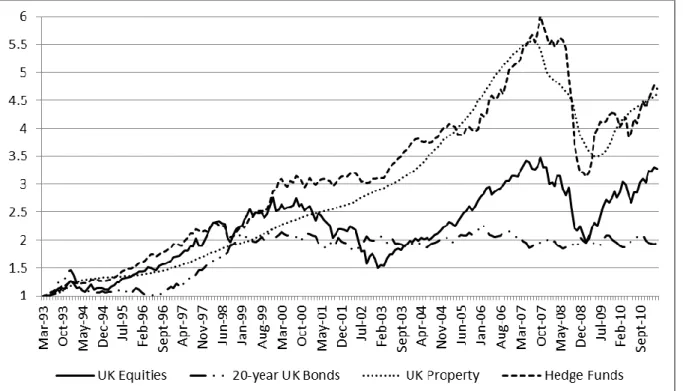
Its maximin objective means that robust optimization will tend to perform better than the other techniques when the market falls; while the USS benchmark with its high equity investment will tend to perform better in a rising market. Figure 1 shows that the data period (1993-2011) covers a wide range of economic conditions, with three strong upward trends in the UK equity market, and two substantial falls. Property and hedge funds show a rise until mid-2007 followed by a sharp fall, and then a rise, while 20 year bond prices rise in the late 1990s and are then fairly steady. This suggests that the results below are not due to testing the ALM models on a falling market, which
16
would favour robust optimization and penalize USS. Indeed, over the entire data period, an investment in the FTSE index basket rose by more than 200%, and hedge funds and property rose by an even larger percentage.
Type Source
Asset Classes
UK Equities FTSE All Share Total Return
EU Equities MSCI Europe excl. UK Total Return
US Equities S&P500 Total Return
10 year UK Bonds 10-year UK Gov. Yields
20 year UK Bonds 20-year UK Gov. Yields
10 year US Bonds 10-year US Gov. Yields
20 year US Bonds 20-year US Gov. Yields
Hedge Funds HFRI Hedge Fund Index
Commodities S&P GSCI Total Return
UK Property IPD Index Total Return
Cash UK 3 Month Treasury Bills
Factors
Global Equities MSCI World Total Return
20 year UK Bonds 20-year Gov. Yields
UK Expected Inflation UK 10-year Implied Inflation
UK Short Term Interest Rate 6-month UK Interbank Rate
Table 1: Dataset for Asset Classes and Factors
17
Figure 1: Cumulative Wealth from an Investment in Each of the Four Main Asset Classes 1993-2011
b. Liabilities. The liabilities were split into three groups - active members, deferred pensioners and pensioners. Changes in their value are driven by changes in four main factors - long-term interest rates, expected salary growth, expected inflation and longevity expectations. The actuarial equations in Board and Sutcliffe (2007) were used to compute the monthly returns for each of the three types of liability (see Appendix D). This was done using monthly 20-year UK government
bond yields6, and the monthly index of UK 10-year implied inflation. The 20-year government bond
yield was used as the discount rate because, while no cash flow forecasts are available, USS is an immature scheme and data on the age distribution of active members, deferreds and pensioners suggests the duration of USS liabilities is over 20 years (USS, 2013). The USS actuary estimates expected salary growth as expected inflation plus one percent, and so monthly changes in expected salary growth were computed in this way. Monthly data on changes in longevity expectations is not available, and so these expectations were held constant throughout each three year period at the value used in the preceding actuarial valuation (see the last two rows of Table 2).
The computation of the liabilities also requires a number of parameters - expected age at retirement, life expectancy at retirement, and the average age of actives and deferreds. Although the USS normal retirement age is 65 years, expected retirement ages are earlier. Row 1 of Table 2 shows the expected retirement ages for actives and deferreds used for each triennial USS actuarial valuation, and row 2 has the expected longevity of USS members at the age of 65 (USS Actuarial Valuations). Since the average age of USS members throughout the period was 46 years (HEFCE, 2010), and the average age of USS pensioners was 70 years (USS, 2013), the number of years for which each group was expected to receive a pension are also shown in rows 3 and 4 of Table 2.
The USS accrual rate in the final salary section is 1/80th per year. In addition there is a lump sum
payment, and using the USS commutation factor of 16:1, this increases the accrual rate to 1/67.37.
6
This abstracts from the effects on returns of the low liquidity of pension liabilities and the inflation risk inherent in government bond yields, as these effects tend to cancel out.
18
Expected Values in Years 1993/6 1996/9 1999/02 2002/5 2005/8 2008/11
Retirement Age 60 60 60 60 60 62
Longevity at 65 20 20 21 21 21 24
Pension Period - Actives & Deferreds 25 25 26 26 26 27 Pension Period – Pensioners 15 15 16 16 16 19
Table 2: Demographic Data for Actives, Deferreds and Pensioners
Expected retirement age for active and deferred members, expected longevity at age 65, expected number of years for which current active and deferred members and pensioners will receive a pension
c. Constraints. The upper and lower bounds on the asset proportions of the five main asset classes were set so as to rule out extreme and unacceptable asset proportions. This was done with reference to the benchmarks and the associated permitted active positions specified by USS over the data period. The bounds used were: (35% ≤ Equities ≤ 85%); (5% ≤ Fixed Income ≤ 30%); (0% ≤ Alternative Assets ≤ 30%); (2% ≤ Property ≤ 15%): and (0% ≤ Cash ≤ 5%). In addition, the expected return on the asset-liability portfolio was required to be non-negative, and short sales and borrowing were excluded.
Actuarial valuations of USS are carried out every three years, with the oldest available actuarial
valuation on 31st March 1993, and the most recent valuation on 31st March 2011. The data is
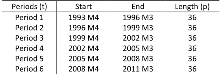
divided into six non-overlapping periods to coincide with these seven triennial actuarial valuations, as shown in Table 3.
Periods (t) Start End Length (p)
Period 1 1993 M4 1996 M3 36 Period 2 1996 M4 1999 M3 36 Period 3 1999 M4 2002 M3 36 Period 4 2002 M4 2005 M3 36 Period 5 2005 M4 2008 M3 36 Period 6 2008 M4 2011 M3 36
Table 3: Non-Overlapping Three Year Data Periods
The data is divided into six 3-year periods corresponding to USS actuarial valuations
19
USS is a very long term investor and sets its asset allocation every three years after conducting an actuarial valuation and commissioning an asset-liability study. Therefore we have used a three year out-of-sample period, together with a six year estimation period. The robustness checks in section 6 include a one year out-of-sample period with a three year estimation period. The data for the initial six years (periods one and two) was used to compute the optimal robust optimization asset allocation for the subsequent three years (period three). The data period was then rolled forward by 36 months, so that data for periods two and three was now used to compute the optimal asset allocation, which was tested on data for period four, and so on, giving four out-of-sample test periods of 36 months each, providing 144 out-of-sample months.
Each of the three liabilities was treated as a separate risky ‘asset class’ with ‘negative’ and fixed weights for each of the six three year periods. We calculated the proportions for each type of pension liability from the triennial actuarial valuations (see Table 4). For the six year estimation periods we used the average of the liability weights for the two 3-year periods concerned. In computing returns on the asset and liability portfolios, the assets were weighted by the funding ratio at the start of the relevant three year period.
Type Period 1 Period 2 Period 3 Period 4 Period 5 Period 6
Active 59.50% 57.42% 55.23% 57.36% 52.51% 52.20%
Pensioners 36.05% 36.25% 37.89% 35.01% 39.56% 39.90%
Deferred 4.45% 6.33% 6.88% 7.63% 7.93% 7.90%
Table 4: Proportions of Total Pension Liabilities
d. Uncertainty Sets. For each estimation period, we calculated the parameters involved in the three uncertainty sets, and hence in the final mathematical optimization problem, using a factor model (equation 1). The returns uncertainty set requires the estimation of 14 mean returns, and for each estimation period the means of the 14 asset and liability returns were used. For each of the six year estimation periods natural log returns on the 11 assets and three liabilities were separately regressed on the natural log returns of the four factors listed in the lower section of Table 1, together with a constant term. These 14 regressions per estimation period generated 56 estimated coefficients (the factor loadings matrix) and 14 constant terms. In total, the factor
20
loadings uncertainty set requires the estimation of 56 coefficients and 10 covariances. The disturbances uncertainty set has 14 parameters, and these were estimated using the residuals from the regressions. The modified Sharpe and Tint model requires 105 elements of the covariance matrix to be estimated. So overall this benchmark requires the estimation of (105+14) = 119 stochastic parameters per estimation period; while robust optimisation needs (56+10+14+14) = 94 stochastic parameters; a reduction of over 20%.
Bayes-Stein requires the estimation of 105 elements of the asset-liability covariance matrix, 14 elements of the mean asset-liability portfolio returns, as well as the estimation of the parameters
g and μA,L,min (see section 2 for more details). Hence, the Bayes-Stein approach requires in total
the estimation of (105+14+2) = 121 parameters per estimation period; 29% more than robust optimization. Black-Litterman requires the estimation of 105 elements of the asset-liability covariance matrix, the weights of the reference asset-liability portfolio (14), the vector of the investor’s views (14), the overall level of confidence in the views (1), the factor that measures the reliability of the implied return estimates (1) and the reliability of each view (14); giving a total of 149 parameters to be estimated, or 59% more than robust optimization.
The factor model requires us to choose the number and identity of the factors, and we experimented with both the identity and number of factors before settling on those listed in Table 1. It is helpful if the ratio of the number of factors to the number of assets and liabilities is small. In previous robust optimization studies this ratio is 0.080 and 0.233 (Goldfarb & Iyengar, 2003); 0.125 and 0.238 (Ling & Xu, 2012) and 0.200 (Glasserman & Xu, 2013). With four factors and 14 assets and liabilities we have a ratio of 0.286, which is higher than previous studies. Five factors would increase the total number of parameters to be estimated by 19 and increase this ratio to 0.357, which would be appreciably higher than any previous study. Therefore we settled on a parsimonious model of four factors.
We chose 20 year UK government bond prices as one of the factors because the discount rate is a key determinant of the value of the three liabilities. It also helps to explain the prices of the four long term government bonds. We included the UK 10 year implied inflation rate as a factor
21
because it is another important determinant of the three liabilities, and also helps to explain asset returns. The MSCI World Total Return index was added to explain returns on the three equity indices and, to a lesser extent, returns on the three alternative assets. Finally we used the 6 month
UK interbank rate as the fourth factor to explain cash and other asset returns. The R2 values in
Table 5 show that these four factors do a good job in explaining returns for all of the 14 assets and liabilities. In section 6 we present robustness checks where we use three different factors.
The adjusted R2 values and significance of these 14 regressions for the entire data set appear in
Table 5 (the results for each of the four 72 month estimation periods were broadly similar). This
shows that for all the assets and liabilities, an F-test on the significance of the equation was
significant at the 0.1% level, and the adjusted R2 s were generally high. The 100% adjusted R2 for
20 year UK bonds is because 20 year UK bonds was one of the four factors included in the factor model.
The equations in Appendix B were then used to compute the three uncertainty sets. Robust
optimisation requires a value of ω to be chosen. Previous authors have used a value of ω = 0.99
(e.g. Delage and Mannor, 2010; Kim, Kim, Ahn and Fabozzi, 2013; and Ling and Xu, 2012) and we
also set ω = 0.99. We experimented with other values of ω, such as 0.90 and 0.95, and obtained
broadly similar results (see section 6). The value of ω was not set equal to unity because the
required confidence level would become infinite.
1993-2011 Adj.R2 % p-value UK Equities 33.34 0.000 EU Equities 91.04 0.000 US Equities 94.88 0.000 10 year UK Bonds 82.64 0.000 20 year UK Bonds 100.00 0.000 10 year US Bonds 43.90 0.000 20 year US Bonds 41.06 0.000 Hedge Funds 79.76 0.000 Commodities 40.90 0.000 UK Property 24.63 0.000 Cash 42.97 0.000 Actives 93.33 0.000 Deferreds 93.45 0.000
22
Pensioners 93.34 0.000
Table 5: Adjusted R2 and Significance Levels of the 14 Regression Equations
Monthly returns on each of the assets and liabilities for 1993 to 2011 were regressed on monthly returns of four factors. These are the MSCI World total return index, the 20 year UK bonds, the implied UK 10 year inflation rate and the UK 6 month interbank rate.
5. Results
The asset allocations for robust optimization and the four benchmarks for the four out-of-sample
periods appear in Table 67. This shows that, while the robust optimization solutions are subject to
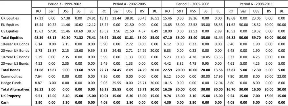
upper and lower bounds on the asset proportions, these constraints are never binding. However varying these bounds changes the optimal solutions because the robust counterpart is a nonlinear convex optimisation problem, and its optimal solution need not be at a corner point. Therefore the solutions were affected by the upper and lower bounds. Sharpe and Tint, Bayes-Stein and Black-Litterman are constrained in every period by the upper bound of 15% on property. In periods 4 and 5 Sharpe and Tint and Bayes-Stein are constrained by the lower bound on equities of 35%, while in period 5 Sharpe and Tint, Bayes-Stein and Black-Litterman are constrained by the upper bound of 30% on alternatives. In section 6 we examine the effects of relaxing these bounds.
7
The robust optimization ALM model was solved using SeDuMi 1.03 within MATLAB (Sturm, 1999), and this took 0.67 seconds for each out-of-sample period on a laptop computer with a 2.0 GHz processor, 4 GB of RAM and running Windows 7. The modified Sharpe and Tint model was solved using the fmincon function in MATLAB for constrained nonlinear optimization problems (interior point algorithm) and took less than a second, as did the Bayes-Stein and Black-Litterman models.
23
Period 3 - 1999-2002 Period 4 - 2002-2005 Period 5 - 2005-2008 Period 6 - 2008-2011
RO S&T USS BS BL RO S&T USS BS BL RO S&T USS BS BL RO S&T USS BS BL UK Equities 17.33 0.00 57.38 0.00 24.91 18.13 31.44 38.81 30.43 26.51 15.46 0.00 38.36 0.00 0.00 18.68 0.00 23.06 0.00 0.00 EU Equities 15.44 10.22 11.46 10.62 12.12 13.27 0.00 21.50 0.00 0.00 13.65 35.00 22.52 35.00 38.55 11.62 50.00 18.32 50.00 50.00 US Equities 15.63 57.91 11.46 60.69 38.37 15.52 3.56 21.50 4.57 8.49 18.00 0.00 22.52 0.00 2.89 16.52 0.00 18.32 0.00 0.00 Total Equities 48.39 68.13 80.30 71.32 75.41 46.92 35.00 81.81 35.00 35.00 47.10 35.00 83.40 35.00 41.44 46.82 50.00 59.70 50.00 50.00 10-year UK Bonds 6.14 0.00 2.15 0.00 0.00 5.90 0.00 2.72 0.00 0.00 6.12 0.00 0.22 0.00 0.00 6.46 0.00 1.90 0.00 0.00 20-year UK Bonds 5.73 13.87 2.15 13.68 9.59 5.33 24.45 2.71 24.29 20.00 6.83 0.00 0.22 0.00 0.00 6.48 0.00 1.90 0.00 0.00 10-Year US Bonds 5.29 0.00 2.35 0.00 0.00 5.99 0.00 1.33 0.00 0.00 5.23 11.18 4.78 10.05 13.56 5.32 0.00 4.25 0.00 0.00 20-year US Bonds 4.52 0.00 2.35 0.00 0.00 5.49 0.00 1.33 0.00 0.00 4.42 8.82 4.78 9.95 0.00 4.61 5.00 4.25 5.00 5.00 Total Bonds 21.68 13.87 9.00 13.68 9.59 22.71 24.45 8.09 24.29 20.00 22.59 20.00 10.00 20.00 13.56 22.87 5.00 12.30 5.00 5.00 Commodities 7.64 0.00 0.00 0.00 0.00 7.26 0.00 0.00 0.00 0.00 6.12 30.00 0.00 30.00 17.96 7.90 30.00 8.00 30.00 22.00 Hedge Funds 8.87 3.00 0.00 0.00 0.00 9.03 25.55 0.00 25.71 30.00 10.15 0.00 0.00 0.00 12.04 8.80 0.00 8.00 0.00 8.00 Total Alternatives 16.52 3.00 0.00 0.00 0.00 16.29 25.55 0.00 25.71 30.00 16.26 30.00 0.00 30.00 30.00 16.70 30.00 16.00 30.00 30.00 UK Property 9.51 15.00 8.40 15.00 15.00 10.01 15.00 8.30 15.00 15.00 9.74 15.00 3.10 15.00 15.00 9.54 15.00 7.00 15.00 15.00 Cash 3.90 0.00 2.30 0.00 0.00 4.08 0.00 1.80 0.00 0.00 4.30 0.00 3.50 0.00 0.00 4.08 0.00 5.00 0.00 0.00
Table 6: Asset Proportions for Robust Optimization (RO), Sharpe and Tint (S&T), USS, Bayes-Stein (BS) and Black-Litterman (BL)
Six year estimation period and 144 months out-of-sample. Optimal asset allocations for each of the four out-of-sample 36 month
24
Table 6 shows that robust optimization leads to remarkably stable asset proportions across the 12 out-of-sample years, with between 47% and 48% in equities, 22% to 23% in bonds, 4% in cash, 10% in property, and between 16% and 17% in alternatives. The asset allocations for the four benchmarks are much more variable. The modified Sharpe and Tint asset allocations vary for equities between 35% and 68%, bonds between 5% and 24%, and alternatives between 3% and 30%. Property is always constrained at the upper bound of 15%, and cash is always constrained at the lower bound of zero. The Bayes-Stein and Black-Litterman allocations also show considerable variability. For example the Bayes-Stein and Black-Litterman allocation to alternatives varies from zero to 30%, while bond allocations vary from 5% to over 20%. The USS allocations are also variable. For the first three periods USS had over 80% of the assets invested in equities, with no investment in alternative assets until the last period, when it jumped to 16% and the equity proportion fell to 60%.
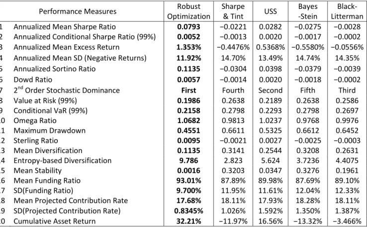
Table 7 compares the results for the five methods over the 144 out-of-sample months. The 144 months comprised the four out-of-sample 36 month periods, with different solutions applying for each 36 month period. Where relevant, the monthly figures were adjusted to give annualized figures. In Table 7 the score for the technique with the best performance on each measure is in bold. Robust optimization is the best technique on all the performance measures.
The Sharpe ratio is the mean excess return on the asset-liability portfolio divided by the standard deviation of returns of the asset-liability portfolio. Since the Sharpe ratio uses the standard deviation to measure risk, to provide an alternative perspective we also used a wide range of additional performance measures which do not rely on the standard deviation. The annualized conditional Sharpe ratio (Eling and Schuhmacher, 2007) is computed at the 99% level, and the
annualized mean excess return is the mean of the asset minus liability returns.The Sortino ratio is
the mean return on the asset-liability portfolio, divided by the standard deviation of returns on the asset-liability portfolio computed using only negative returns, with the minimum acceptable return set to zero (Prigent, 2007). The Dowd ratio is the mean return on the asset-liability portfolio, divided by the value at risk for a chosen confidence level (deflated by the initial value of
25
the asset-liability portfolio), (Prigent, 2007). We used the 99% confidence level for the value at risk when computing the Dowd ratio, and have also included the value at risk and the conditional value at risk, both at the 99% level, in Table 7 as measures of tail risk. Another distribution-free performance measure - second order stochastic dominance - is also included in Table 7.
Performance Measures Robust Optimization
Sharpe
& Tint USS
Bayes -Stein
Black- Litterman 1 Annualized Mean Sharpe Ratio 0.0793 −0.0221 0.0282 −0.0275 −0.0028 2 Annualized Conditional Sharpe Ratio (99%) 0.0052 −0.0013 0.0020 −0.0017 −0.0002 3 Annualized Mean Excess Return 1.353% −0.4476% 0.5368% −0.5580% −0.0556% 4 Annualized Mean SD (Negative Returns) 11.92% 14.70% 13.49% 14.74% 14.35% 5 Annualized Sortino Ratio 0.1135 −0.0304 0.0398 −0.0379 −0.0039 6 Dowd Ratio 0.0057 −0.0014 0.0020 −0.0018 −0.0002 7 2nd Order Stochastic Dominance First Fourth Second Fifth Third 8 Value at Risk (99%) 0.1986 0.2638 0.2189 0.2638 0.2586 9 Conditional VaR (99%) 0.2158 0.2798 0.2293 0.2798 0.2697 10 Omega Ratio 1.0682 0.9813 1.0237 0.9768 0.9976 11 Maximum Drawdown 0.4551 0.6611 0.5325 0.6612 0.6452 12 Sterling Ratio 0.0095 −0.0021 0.0027 −0.0025 −0.0003 13 Mean Diversification 0.1135 0.3141 0.2544 0.3208 0.2631 14 Entropy-based Diversification 9.786 2.823 5.624 3.7236 4.4075 15 Mean Stability 0.0016 0.3203 0.0347 0.3276 0.1961 16 Mean Funding Ratio 93.01% 87.89% 89.98% 87.69% 89.10% 17 SD(Funding Ratio) 9.700% 11.95% 11.61% 12.04% 12.33% 18 Mean Projected Contribution Rate 17.68% 18.11% 17.93% 18.28% 18.11% 19 SD(Projected Contribution Rate) 0.8345% 1.026% 1.592% 1.350% 1.387% 20 Cumulative Asset Return 32.21% −11.97% 16.56% −13.32% −3.466%
Table 7: Out-of-Sample Performance Measures – Six Year Estimation Period
The results for each of the four out-of-sample 36 month periods were adjusted, where relevant, on to an annualised basis. The original bounds, assets, factors and constraints were used, and ω = 0.99.
The Omega ratio is the ratio of the average gain to the average loss, and is an additional distribution-free measure of performance (Bessler, Opfer and Wolff, forthcoming). Gains are the positive excess returns of assets over liabilities, and losses are the negative excess returns of assets over liabilities. The drawdown rate, which is also distribution-free, measures declines from
peaks in cumulative wealth over a specific time horizon (t). The drawdown rate is defined as:-
0 0 max W W DD max W τ t τ t t τ τ t (12)where Wt is the cumulative wealth (assets only) at time t. Maximum drawdown is the largest
26
comparison with others, it tends to have lower volatility and value-at-risk. We also included some further performance measures based on the drawdown rate. The Sterling ratio is the mean asset return divided by the average drawdown rate (Eling and Schuhmacher, 2007).
Diversification of the asset-only portfolios was measured as the average across the four periods of the sum of the squared portfolio proportions for each period (Blume and Friend, 1974). For zero
diversification the score is one, while for full diversification it is 1/nA (or 0.091 when nA = 11).
Following Bera and Park (2008) we also used entropy to measure asset diversification. We
modified Shannon’s entropy by taking its exponent giving the measure Z in equation (13), so that
for zero diversification Z = 1, and for full diversification Z =nA, (which is 11).
A A, A, 1 ln n i i i Z exp
(13)The stability of portfolio proportions from one triennial period to the next was measured as the average value across the three changes in asset allocation of the sum of squares of the differences between the portfolio proportion for each asset in adjacent time periods (Goldfarb and Iyengar, 2003). This measure can be viewed as a proxy for transactions costs under the assumption that the cost functions are linear and similar across assets. Robust optimization adopts a maximin objective, and with an ω value of 0.99, it selects portfolios that are very likely to deliver at least their expected Sharpe ratio. Therefore it is pessimistic, tending to select very cautious portfolios. During bull markets it still selects portfolios that will deliver at least the expected Sharpe ratio, even if there is a market downturn. Thus robust optimization asset allocations tend to be more stable than those of other asset selection techniques. Our stability results are in accordance with the literature. For instance, Gulpinar and Pachamanova (2013) and Goldfarb and Iyengar (2003) report that the size of changes in asset proportions is smaller for the robust portfolio formulation than for the classical approaches. The use of a four factor model, rather than 14 assets and liabilities, may also play a role in ensuring the stability of the robust optimization portfolios.
The monthly out-of-sample asset and liability returns, in conjunction with the values of USS assets and liabilities at the previous actuarial valuation, were used to compute the funding ratio each
27
month. These monthly ratios were averaged to give the mean funding ratio. The mean projected contribution rate was computed using the actuarial formulae in Board and Sutcliffe (2007) with a
spread period (M) of 15 years (see Appendix A). The number of years accrued by the average
member (P) was 18 years, while administrative expenses were set to zero. The term NAS cancels
out with terms in ALA. The values of the discount rate (d’) and salary increase (e) were the average
values over the preceding two triennial periods. Finally the cumulative returns over the 144 out-of-sample months in Table 7 are for just the asset portfolio.
6. Robustness Checks
We varied the base case above along six dimensions. For each robustness check except the last we changed one aspect of the base case, while keeping the others at their values in the base case. We:- (i) reduced the estimation period from six to three years; (ii) used two alternative sets of factors in the robust optimization - in the first set UK expected inflation was replaced by RPI, and in the second set UK 6 month rates were replaced by UK 3 month rates, UK 20 year bonds by UK 10 year bonds, and UK expected inflation by RPI; (iii) the S&P GSCI total return index was replaced by the S&P GSCI Light Energy total return index, and UK private equity and UK infrastructure were
included as alternative assets, replacing 20 year UK and US bonds; (iv) ω was reduced from 0.99 to
0.90; (v) the upper and lower bounds on the asset allocations were relaxed by 5%, becoming (30% ≤ equities ≤ 90%); (0% ≤ fixed income ≤ 35%); (0% ≤ alternative assets ≤ 35%); (0% ≤ property ≤ 20%): and (0% ≤ cash ≤ 10%), and (vi) the estimation period was reduced to three years and the out-of-sample period was reduced to one year.
Bessler, Opfer and Wolff (forthcoming) suggest that the reliability of the views incorporated in the Black-Litterman model is time-varying. For each of our out-of-sample periods in Table 7 we estimated the reliability of the views for the subsequent out-of-sample period using the entire estimation period of 72 months. As a further robustness check, we compared the base case with five versions of the Black-Litterman model where we used the 12, 18, 24, 30 and 36 months immediately prior to the start of each out-of-sample period to estimate the reliability of the views,
28
measured as the variance of the historic forecast errors. For all five of these shorter estimation periods, robust optimization remains superior on every performance measure.
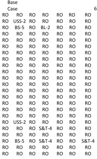
The results for these six alternative formulations of the problem are summarised in Table 8. For the base case and the six alternative cases, the best technique for each performance measure is indicated. Where robust optimization is not the best technique, Table 8 also shows the ranking of robust optimization.
Performance Measures Base
Case 1 2 3 4 5 6
1 Annualized Me