Computational intelligent hybrid model for detecting disruptive trading activity

for detecting disruptive trading activity

Zhai, J, Cao, Y, Yao, Y, Ding, X and Li, Y

http://dx.doi.org/10.1016/j.dss.2016.09.003

Title

Computational intelligent hybrid model for detecting disruptive trading 

activity

Authors

Zhai, J, Cao, Y, Yao, Y, Ding, X and Li, Y

Type

Article

URL

This version is available at: http://usir.salford.ac.uk/40197/

Published Date

2016

USIR is a digital collection of the research output of the University of Salford. Where copyright 

permits, full text material held in the repository is made freely available online and can be read, 

downloaded and copied for non­commercial private study or research purposes. Please check the 

manuscript for any further copyright restrictions.

For more information, including our policy and submission procedure, please

contact the Repository Team at: 

[email protected]

.

Computational intelligent hybrid model for detecting disruptive trading activity

Jia Zhai, Yi Cao, Yuan Yao, Xuemei Ding, Yuhua Li PII: S0167-9236(16)30152-X DOI: doi:10.1016/j.dss.2016.09.003 Reference: DECSUP 12760

To appear in: Decision Support Systems Received date: 14 December 2015 Revised date: 18 August 2016 Accepted date: 9 September 2016

Please cite this article as: Jia Zhai, Yi Cao, Yuan Yao, Xuemei Ding, Yuhua Li, Com-putational intelligent hybrid model for detecting disruptive trading activity, Decision Support Systems(2016), doi: 10.1016/j.dss.2016.09.003

This is a PDF file of an unedited manuscript that has been accepted for publication. As a service to our customers we are providing this early version of the manuscript. The manuscript will undergo copyediting, typesetting, and review of the resulting proof before it is published in its final form. Please note that during the production process errors may be discovered which could affect the content, and all legal disclaimers that apply to the journal pertain.

ACCEPTED MANUSCRIPT

1

Computational intelligent hybrid model for detecting disruptive trading activity

All Authors: Jia Zhai,

Salford Business School, University of Salford, Salford, M5 4WT, UK

Yi Cao,

Division of Mathematics and Computation, School of Computing, Mathematics and Digital Technology Manchester Metropolitan University, Manchester, M1 5GD, UK

Yuan Yao,

Institute of Management Science and Engineering, School of Business Administration

Henan University, 475004, Jinming District, Kaifeng, China

Xuemei Ding,

Faculty of Software, Fujian Normal University, 350108, Fuzhou, Fujian Province, China

Yuhua Li,

ACCEPTED MANUSCRIPT

2 Corresponding author:

Yuan Yao

Institute of Management Science and Engineering, School of Business Administration

Henan University, 475004, Jinming District, Kaifeng, Henan Province, China Email: [email protected]

Abstract

The term “disruptive trading behaviour” was first proposed by the U.S. Commodity Futures Trading Commission and is now widely used by US and EU regulation (MiFID II) to describe activities that create a misleading appearance of market liquidity or depth or an artificial price movement upward or downward according to their own purposes. Such activities, identified as a new form of financial fraud in EU regulations, damage the proper functioning and integrity of capital markets and are hence extremely harmful. While existing studies have explored this issue, they have, in most cases, either focused on empirical analysis of such cases or proposed detection models based on certain assumptions of the market. Effective methods that can analyse and detect such disruptive activities based on direct studies of trading behaviours have not been studied to date. There exists, accordingly, a knowledge gap in the literature. This paper seeks to address that gap and provides a hybrid model composed of two data-mining-based detection modules that effectively identify disruptive trading behaviours. The hybrid model is designed to work in an on-line scheme. The limit order stream is transformed, calculated and extracted as a feature stream. One detection module, “Single Order Detection,” detects disruptive behaviours by identifying abnormal patterns of every single trading order. Another module, “Order Sequence Detection,” approaches the problem by examining the contextual relationships of a sequence of trading orders using an extended hidden Markov model, which identifies whether sequential changes from the extracted features are manipulative activities (or not). Both models were evaluated using huge volumes of real tick data from the NASDAQ, which demonstrated that both are able to identify a range of disruptive trading behaviours and, furthermore, that they outperform the selected traditional benchmark models. Thus, this hybrid model is shown to make a substantial

ACCEPTED MANUSCRIPT

3 contribution to the literature on financial market surveillance and to offer a practical and effective approach for the identification of disruptive trading behaviour.

Keywords:

ACCEPTED MANUSCRIPT

4

Computational intelligent hybrid model for detecting disruptive trading activity

Abstract

The term “disruptive trading behaviour” was first proposed by the U.S. Commodity Futures Trading Commission and is now widely used by US and EU regulation (MiFID II) to describe activities that create a misleading appearance of market liquidity or depth or an artificial price movement upward or downward according to their own purposes. Such activities, identified as a new form of financial fraud in EU regulations, damage the proper functioning and integrity of capital markets and are hence extremely harmful. While existing studies have explored this issue, they have, in most cases, either focused on empirical analysis of such cases or proposed detection models based on certain assumptions of the market. Effective methods that can analyse and detect such disruptive activities based on direct studies of trading behaviours have not been studied to date. There exists, accordingly, a knowledge gap in the literature. This paper seeks to address that gap and provides a hybrid model composed of two data-mining-based detection modules that effectively identify disruptive trading behaviours. The hybrid model is designed to work in an on-line scheme. The limit order stream is transformed, calculated and extracted as a feature stream. One detection module, “Single Order Detection,” detects disruptive behaviours by identifying abnormal patterns of every single trading order. Another module, “Order Sequence Detection,” approaches the problem by examining the contextual relationships of a sequence of trading orders using an extended hidden Markov model, which identifies whether sequential changes from the extracted features are manipulative activities (or not). Both models were evaluated using huge volumes of real tick data from the NASDAQ, which demonstrated that both are able to identify a range of disruptive trading behaviours and, furthermore, that they outperform the selected traditional benchmark models. Thus, this hybrid model is shown to make a substantial contribution to the literature on financial market surveillance and to offer a practical and effective approach for the identification of disruptive trading behaviour.

1.

Introduction

Trading surveillance for the monitoring of disruptive trading activities with “intent to mislead the market” has been a topic of interest for regulators in recent years, especially after the flash crash in 2010 (CME, 2014) (EU, 2014)

ACCEPTED MANUSCRIPT

5 (Domowitz, 2012) (Friederich & Payne, 2012). The term “disruptive trading behaviours” was first proposed by the US Commodity Futures Trading Commission (CFTC) in 2013 in their interpretive statement (CFTC, May 20 2013) to prohibit certain disruptive trading, practices, or conduct defined as: bids or offers with intent to cancel the bid or offer before execution for violating the bid or offer prices with reckless disregard for the orderly execution or market integration. This concept has also attracted much attention from the regulators in other exchanges in the USA and EU. The Chicago Mercantile Exchange (CME) released a “Rule 575” on August 28, 2014 (CME, 2014) to add “certain of the disruptive practices” to the CFTC interpretive statement (CFTC, May 20 2013). In “Rule 575,” disruptive practices are further defined as orders with the purpose to cancel or mislead other market participants or to disrupt the exchange or other fair executions. In the EU, the Markets in Financial Instruments Directive II (MiFID II) was proposed as legislation regulating firms’ activities in financial markets (EU, 2014). In MiFID II, a market disruptive practice is explained as a form of financial market fraud that includes all types of market abuse and spoofing activities. Due to the lack of existing research and the implementation difficulties, the MiFID II application date has been extended by the European Commission to 3 January 2018 (MOCK & LUPINI, 2016). In academia, disruptive trading activities were first introduced by Allen (Allen & Gale, 1992) as trade-based manipulation, which was carried out by carefully designed selling and buying sequences to induce market prices to move and follow their expectations to make a profit. The profitability and the market effects of such disruptive trading activities were then studied in (Aggarwal & Wu, 2006) and (Aitken, Harris, & Ji, 2009), respectively. Subsequently, traditional data mining approaches have been studied to identify disruptive trading activities in (Öğüt, Doğana, & Aktaş, 2009), (Mongkolnavin & Tirapat, 2009), (Diaz, Theodoulidis, & Sampaio, 2011), and (Cao Y. , Li, Coleman, Belatreche, & McGinnity, 2015). However, those studies mainly focus on particular forms of market manipulation or disruptive behaviours rather than a complete study. In general, unlike the financial fraud in traditional areas, i.e., financial statements (Ravisankar, Ravi, Rao, & Bose, January 2011) and credit cards (Bhattacharyya, Jha, Tharakunnel, & Westland, February 2011), which have been thoroughly studied, the fraud format of disruptive trading has been less studied. Ngai et al. (Ngai, Hu, Wong, Chen, & Sun, February 2011) found a distinct lack of research on securities and commodities fraud, which is another term for disruptive behaviours and market manipulation. Consequently, the study of disruptive trading and its detection is important and necessary due to the requirements of regulation around the world. This study contributes to the literature

ACCEPTED MANUSCRIPT

6 gap in the financial fraud area as well as the urgent requirements from financial decision-makers, i.e., regulators around the world.

Disruptive trading behaviours can be carried out by either a single buy or sell order or a series of trading actions. Therefore, a thorough monitoring of disruptive trading shall be on each single trading action and a sequence of actions linked in contextual relationships. This is the main challenge of such a disruptive trading behaviour-monitoring problem. Another challenge arises from the fact that the trading data are usually non-stationary, and the existing regulations merely provide qualitative guidance regarding what constitutes “disruptive” instead of a quantitative definition. Most of the existing related literature empirically studies the corresponding market responses when experiencing disruptive trading. Very few works analyse the features of disruptive trading behaviours and the

corresponding detection approaches. Our paper contributes to the literature gap via a thorough study of the behaviours of disruptive trading and the proposal of a hybrid detection model. A number of disruptive trading forms, i.e., ramping, spoofing, spoofing and layering, and quote stuffing, have been summarized and studied in recent years after the flash crash (Cumming, Zhan, & Aitken, 2013). The former two forms, ramping and spoofing, are essentially the same form: placing large-sized or aggressively priced orders individually on the market to create the appearance of an unbalanced order book. We name it “Single Order Disruptiveness” since the spoofing orders are placed separately with no linked relations. The latter two forms, spoofing and layering and quote stuffing, are usually to overload the quotation system with large numbers of sequential aggressively priced bids or offers (Lee, Eom, & Park, 2013) (CME, 2014) (EU, 2014). Therefore, we name it “Multi Order Disruptiveness” since the spoofing is carried out by contextually linked orders. The impact of “Single Order Disruptiveness” is associated with the aggressive features of one single order, and the impact of “Multi Order Disruptiveness” depends on the contextual relationship among the order sequences. Therefore, to effectively identify both tactics, we need a model that captures both the single and contextual features of orders. Until now, the existing research has fallen into two categories. The first category, empirical studies of

disruptive trading activities, proves the damage of disruptive trading to the proper functioning and integrity of capital markets. The second category is detection model designs based on an arguable assumption: that abnormal changes of market variables, i.e., daily return, trading volume and daily volatility, indicate disruptive trading activities. Market variable changes can be induced by disruptive trading activities, but in most cases are changed by economic or other

ACCEPTED MANUSCRIPT

7 events. Therefore, an abnormal change of market variables is a necessary but not sufficient condition of disruptive trading. Detection model designs based on that hardly achieve accurate and reliable performance across different markets and time periods.

This study introduces a hybrid detection model using two computational intelligent algorithms, Support Vector Machine (SVM) and Hidden Markov Model (HMM), together with a tailor-made feature extraction approach and an adaptive mechanism. The SVM detects anomalous single orders compared with normal trading behaviours, and the HMM identifies the disruptive impacts caused by contextually sequential orders. Those two models are combined as a hybrid model that covers a complete spectrum of disruptive trading activities regardless of their forms, i.e., ramping, spoofing or quote stuffing. To compensate for the non-stationary nature of the trading behaviours, a straightforward transformation ( ) is proposed as a pre-processing module for the hybrid model. The trading order is converted into a feature space, in which the hybrid model searches and recognises single as well as contextual disruptive patterns that depart from ordinary trading behaviours.

To the best of our knowledge, the proposed hybrid model, which completely detects and recognises disruptive trading activities based on a thorough analysis of the trading features, has not previously been presented. Substantial

experiments have been conducted on very recent real data from US markets to evaluate the performance of the proposed framework against selected popular machine learning algorithm benchmarks. The rest of the paper is organised as follows: Section 2 provides a review of all relevant literatures; Section 3 begins with a detailed

explanation of the problem and a formulation of typical cases. The hybrid detection model is proposed and discussed in detail in Section 4, and Section 5 presents the paper’s conclusions.

2.

Relevant Literature

Disruptive trading activities were first defined and discussed by Allen as trade-based manipulation, which is carried out only by carefully designed selling and buying sequences to induce market prices to move and follow their expectations (Allen & Gale, 1992). In his work, Allen also introduced a theoretical framework of trade-based manipulation

ACCEPTED MANUSCRIPT

8 profitability, which is dependent on normal investors’ knowledge of the existence of manipulators. Aggarwal and Wu (Aggarwal & Wu, 2006) carried on from Allen and Gale’s work and looked at profitable trade-based manipulation. They looked at the implication of manipulation on market efficiency and what indices were affected by it and also found that equities with low values and illiquidity were commonly targeted. They found that manipulators can curtail the effectiveness of arbitrage activities and that, during the manipulation period, liquidity, returns and volatility increased. There are fewer works related to the detection of disruptive trading activities in contrast with the volume of theoretical and empirical work on it. One paper explores and compares two computational approaches to the detection of trade-based manipulation in the Istanbul Stock Market. The computational approaches include logistic regression, artificial neural networks, and support vector machine (Öğüt, Doğana, & Aktaş, 2009). In this paper, detection is based on empirical studies of the statistics arising from market variables, including daily return, daily trading volume and daily volatilities. The assumption of the detection is that the greater the deviation of selected market variables from legitimate trading records, the more likely an event is deemed as manipulation. Other studies take similar approaches, for example, by studying known cases of manipulation that have been documented by the Securities and Exchange Commission (SEC) and then constructing a manipulated-cases data set, modelling the returns, liquidity, volatility, relevant news and related events using linear and logistic regression (Diaz, Theodoulidis, & Sampaio, 2011). Aitken et al. (Aitken, Harris, & Ji, 2009) suggested that trade-based price manipulations could have significantly increased the execution costs of larger trades on 34 of the world's exchange markets between 2000 and 2005. Aitken's team refer to just one form of trade-based manipulation, ramping. The actual ramping alerts in the markets at the time were collated by Smarts Group International, which provides market surveillance solutions to the NASDAQ OMX. Exploration of the relationships between price manipulation and market efficiency reveals that (1) manipulation led to increased execution costs for larger trades and (2) the fewer the ramping alerts, the less the magnitude of spreads. Indeed, the result of halving or doubling ramping alerts was a 10% change in execution costs for larger trades across the world. This clearly shows how substantially market efficiency is affected by market integrity, at least in regard to larger trades. Lee et al. (Lee, Eom, & Park, 2013) examined how traders strategically spoofed the stock market by placing orders with little chance of being executed but with significant misleading effect on the appearance of an imbalance in the order book.

ACCEPTED MANUSCRIPT

9 Until now, researchers have focused primarily on detecting manipulation based on assumptions drawn from empirical studies: unusual changes of certain market variables indicate manipulations. Those market variables include the daily return, daily trading volume and daily volatilities (Öğüt, Doğana, & Aktaş, 2009), liquidity (Diaz, Theodoulidis, & Sampaio, 2011), and transaction price, volume and time (Mongkolnavin & Tirapat, 2009). However, there is no proof showing that such unusual changes are a sufficient condition for the manipulation, which means that, although a manipulation may incur changes of market variables, those changes might not be only the results of manipulations and could possibly be results of other events in the market, i.e., big news or an economic cycle. Only two very recent papers discuss the detection of manipulative activities based on trading behaviours (Cao Y. , Li, Coleman, Belatreche, & McGinnity, 2015) (Cao Y. , Li, Coleman, Belatreche, & McGinnity, 2015). However, the proposed models only target certain types of disruptive trading activities, i.e., quote stuffing, by monitoring the most aggressive buy/sell orders, with other orders being ignored.

Therefore, the existing work does not contribute to a theoretical foundation for detecting disruptive trading behaviours. Unlike other related literature, this paper does not address the market manipulation issue but only the disruptive trading. This is because, in the most updated regulation (CME, 2014) (EU, 2014), “manipulation” has been defined as a juristic activity and requires detailed inspections to determine the psychological intentions of a trader’s disruptive behaviours. Therefore, rather than manipulation identification, this paper addresses the detection of disruptive trading behaviours from the limit order streams and covers all primary types of disruptive patterns, which are through either single or multiple orders. To the best of our knowledge, this is the first study regarding the detection of disruptive trading behaviours that are based on trading order streams, covering all primary types of disruptiveness. This paper, on one hand, contributes to the literature regarding decision-making for the financial market regulation and, on the other hand, also contributes to the literature on the financial market to fill the gap regarding market manipulation behaviour studies (Lee, Eom, & Park, 2013) (Aitken, Harris, & Ji, 2009) and trading behaviour surveillance.

ACCEPTED MANUSCRIPT

10

3.

Problem Formulation

In capital markets, traders submit limit orders to the exchange market with intentions of buying or selling volumes of a specific equity at a given price. When those bona fide limit orders are matched, they are executed. If not, orders are outstanding on the exchange market as the order book. Alternately, some traders also submit limit orders to the market with no intention of execution but to mislead other traders on the market so that they may yield a profit from the counterparts. The activity of submitting such non-bona fide limit orders is usually termed a disruptive trading

behaviour (CME, 2014) (EU, 2014). Disruptive trading behaviours can be carried out by a single order or a sequence of multiple orders, both of which have different features and different impacts on the market. Therefore, we discuss them separately in the following sections.

3.1

Single-order disruptive trading

Some trader use straight-forward disruptive trading tactic to mislead the market. The forms are named obstacle (Cumming, Johan, & Li, 2011), ramping (Tse, Lin, & Vincent, 2012) (EU, 2014), and spoofing (CME, 2014). All of these names essentially refer to the same form: placing a single large-sized or aggressively priced order on the market for a relatively longer time period than that of average orders to create the appearance of a narrowed spread or unbalanced depth on the order book (Hautsch & Huang, 2012) (Lee, Eom, & Park, 2013) (Cao Y. , Li, Coleman, Belatreche, & McGinnity, Mar. 2014). Usually, disruptive trading activity is associated with a legitimate order, placed on the opposite side to the non-bona fide orders in the order book, awaiting execution to make the potential profit. Once the legitimate order is executed (or partially executed), the non-bona fide orders are immediately cancelled. The disruptive trading tactic is what the trader utilises with intent to generate an upward or downward movement in the bid or ask price, and thus further profit-making activity is only undertaken when sufficient potential profit is likely to be generated. Therefore, the disruptive trading tactic is not realized by heuristic attempts but by careful designs of the submitted order under market impact theory, which suggests that the aggressiveness of the quotes and the sizes of placed orders determine the subsequent market effects. Hautsch (Hautsch & Huang, 2012) used a vector autoregressive model (VAR) for quantitative estimation of such effect, which revealed that a notably large size or quote (compared with the current bid or ask) exerted a substantial effect on the market price. Clearly it is crucial for legitimate traders to eliminate those impacts to achieve the best execution price; however, such effects are utilized by traders who use

ACCEPTED MANUSCRIPT

11 disruptive trading to make a profit. Therefore, to maximise the effects on the market for potential profits, the disruptive trading orders should be either large-sized or aggressively priced (much higher or lower than the prevailing bid or ask). However, in practice, obviously huge-sized or aggressively priced trading can be easily suspected as an anomaly by regulators (Hautsch & Huang, 2012) (Lee, Eom, & Park, 2013). Considering this, the traders utilizing disruptive trading actions usually carefully design the trading orders to (1) maximise the price change they may induce and (2) minimise the chance of execution and monitoring.

Lee (Lee, Eom, & Park, 2013) thoroughly studied one type of single-order disruptive trading and termed such a single order as a spoofing order: an order of a size at least twice that of the previous day’s average order size, a price at least 6 bps away from the current bid or ask price and a cancellation time exceeding 30 minutes. In this definition, the

quantitative features of order size (“twice”) and cancellation time (“30 minutes”) are the factors to maximise the market impact for potential profit, and the “6 bps away” helps the order hide from execution and inspection. Similarly, another type of spoofing order is discussed and defined by Hautsch (Hautsch & Huang, 2012) as an order of normal size, a price approximately 6.9 bps inside the spread and a cancellation time of approximately 819 ms. The aggressive price (6.9 bps inside the spread) is to induce the price change, and the short cancellation time is to minimise the risk of execution and inspection. The spoofing orders in single-order disruptive trading are illustrated in Figure 1, where the two above-discussed types of disruptive orders are graphically shown in a three-level order book. The normal-sized and quick-swept orders are aggressively inside the spread, and the passively priced orders are large-sized and stay in the order book for a long time. Clearly, price, size and time staying on the order book are three crucial order features that the traders can tune to achieve their purpose: either normal or disruptive. Although typical features of orders in disruptive trading were defined by Lee (Lee, Eom, & Park, 2013) and Hautsch (Hautsch & Huang, 2012), they do not necessarily follow those definitions and can be variant in different equities across different time periods. Accordingly, identifying the normality or disruptiveness of an order requires accurately modelling their boundaries rather than simply using the thresholds on each of those features.

ACCEPTED MANUSCRIPT

Bid Side Ask Side

Normal size Aggressive price Short cancellation time

Figure 1 single-order disruptive trading

3.2

Multi-order disruptive trading

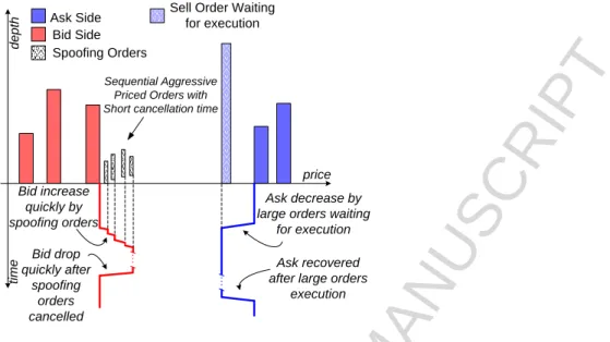
Traders can also submit multiple limit orders as a sequence to the market with no intention of execution. This tactic is termed layering and quote stuffing (Cumming, Zhan, & Aitken, 2013). The two names refer to the identical format: the submission of multiple orders at sequentially increasing or decreasing prices that are higher or lower than the current bid or ask price for spoofing, the submission of another large-sized order on the other side of the order book to make a profits, and the execution of the large-sized order to rapidly remove the previous multiple orders. This tactic usually floods the market with vast quantities of new orders, which are then cancelled in swift succession, thereby creating a succession of new best bid or ask quotes. Each of these quotes has the potential to lure an execution of the opposite order, which may generate a profit. The traders usually carefully design the sequence of orders based on the market impact theory (Hautsch & Huang, 2012). As per the discussion in Section 3.1, Hautsch estimated the market impact such that the aggressive quotes exerted a substantial effect on the market price. A sequence of aggressive quotes certainly induces stronger impacts, from which the trader may make a profit. Figure 2 shows an example of a sequence of spoofing orders in multi-order disruptive trading activities. In this example, with a bona fide large-sized sell order placed at an expected price on the ask side, a succession of manipulative buy orders, with quotes successively higher than the best bid price, were submitted to give the impression of active purchasing interest in that equity. If a trader, encouraged by the (fake) bid price changes, thus responded to the bona fide sell order, and if, just as this was almost executed, the bid quoting orders were all cancelled, the bid price would plummet back to its original level. Such tactics are usually carried out extremely swiftly to minimise the risk of the spoofing orders being picked up by genuine

ACCEPTED MANUSCRIPT

13 investors, and thus with its sequential quotes and speedy cancellations, the spoofing orders in Figure 2 made a saw-tooth-square-shaped market impact upon the bid price.

price d e p th Spoofing Orders Bid Side

Ask Side Sell Order Waiting _{for execution}

ti

m

e

Sequential Aggressive Priced Orders with Short cancellation time

Bid increase quickly by spoofing orders Bid drop quickly after spoofing orders cancelled Ask decrease by large orders waiting

for execution Ask recovered after large orders

execution

Figure 2 Multi-order disruptive trading triggers the bid price to increase quickly and drop also quickly after the spoofing orders are cancelled

4.

Hybrid Detection Model

As per the discussion in Section 3, when carrying out the disruptive trading, a trader utilises the market impact theory to tune the features of limit orders to spoof the market for potential profits. Aggressive (inside spread) price, large size and long time period staying on the order book are features that enhance the market impact. Passive (outside spread) price, normal size and tiny time period on the order book are features that reduce the risk of unconscious execution by other traders and inspections by regulators. The features are summarized in the following Table 1, where the Italic Bold font indicates the features that enhance the market impact and the normal font indicates risk-reducing features.

Table 1 Order features of disruptive trading tactic

Disruptive Trading Price Size Time on order book Single-Order Trading Passive (outside spread) Large Long

Multi-Order Trading Sequentially Aggressive (inside spread) Normal Short

The summary shows the qualitative analysis of the disruptive trading tactics: a certain combination of three features of the limit order is illustrative of the legitimacy or disruptiveness of trading behaviour. Through construction of a feature vector that uses the features of price, volume and time, it is possible to quantitatively model the trading behaviours. This form of presentation can be useful in modelling data regarding trading behaviour, using machine learning

ACCEPTED MANUSCRIPT

14 techniques. However, the non-stationary nature of financial data makes such modelling far more complex. To address this, this paper proposes a transformation method that partially reduces the non-stationarity of the original data. Together with the transformation method, this paper proposes a hybrid model that recognises the disruptive trading behaviours through single orders and multi-order sequences.

4.1

Transformation of original trading data

4.1.1

Proposed Transformation Method

As has been discussed, financial data are usually considered to be a non-stationary time series (Ghazali, Hussain, Nawi, & Mohamad, 2009). Time series analysis, such as the autoregressive integrated moving average (ARIMA) model (which is usually used in cases where the stationary nature of data can be eliminated using an initial differencing step (Tsay, 2010)), echoes this situation. The log return is also regarded as a traditional transformation approach for converting market data to a new time series, which is believed to not be perfectly time invariant (Engle, 1982)

(Bollerslev, 1986) but nonetheless has recently been analysed and determined to be stationary (Lee, Lee, & Lee, 2010). The authors, inspired by both the differencing step and log-return approaches, have defined a transformation procedure that converts the original order data into a new measure. Under this new measure, the data shows a pseudo-stationary feature.

From this section, we take as a time index, which denotes all order book activities (namely submission, cancellation and execution) and then illustrates an incoming order as a vector , with and being the order price, volume and submission time, respectively. Let and indicate the best bid and ask prices instantaneously before the order activity, and is the length of a sliding window for calculating the moving average of the order volume. Given that manipulative behaviour usually occurs within a short time period, is set to one trading day. Thus, the moving average volume of limit orders in the previous time, excluding the current data point , can be represented as

(1)

ACCEPTED MANUSCRIPT

15 Let and represent the cancellation and execution time of a limit order, respectively; we can denote the lifecycle of an order as

(2)

The order execution and cancelation of a limit order are usually correlated with its volume. Therefore, the volume-weighted average lifecycle (VWAL) of limit orders, in the prior period is calculated as

(3)

Therefore, we convert a limit order to a three-dimensional impulse vector by the transformation approach as follows (4) (5) (6)

The three-component impulse measures the aggressiveness of the price, volume and life cycle of a limit order. Because most buy orders are placed at equal to or less than the best bid price, the impulse of the buy orders, termed the buy impulse (BI), is mostly less than or equal to zero. Similarly, the impulse of the sell orders, termed the sell impulse (SI), is mostly higher than or equal to zero.

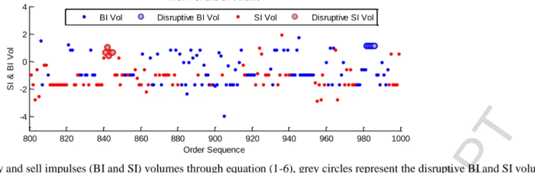
In 24 Jan 2013, two disruptive trading cases on Microsoft (MSFT) stock were reported by Nanex (NANEX, 2013). The original data of the two disruptive trading cases and normal trading data during the same time period are illustrated in Figure 3(a). The red and blue dots represent sell orders (SO) and buy orders (BO), respectively, and the red and blue lines are ask and bid prices, accordingly. The grey filled circles with red or blue edges represent the disruptive sell or buy orders, respectively. It is clearly observed that the disruptive sell orders (red Disruptive SO) around order index 840 are placed inside the spread and sequentially lower the ask price. Similarly, the disruptive buy orders (blue

ACCEPTED MANUSCRIPT

16 Disruptive BO) around order index 980 are placed inside the spread, sequentially raising the bid price and then

narrowing the spread. In addition, we also show the transformed sell (termed SI) and buy (termed BI) order prices of the two disruptive cases as grey filled circles in Figure 3(b) and (c), respectively. It is clear that the disruptive SIs are below zero and are sequentially decreased and that the disruptive BIs, alternately, are above zero and are increased consecutively. The corresponding volumes of the disruptive orders are transformed by equations (1) and (5) and shown in Figure 3(d), where we can also observe the relatively higher volumes of the disruptive orders. The same patterns can also be observed in the reported disruptive trading cases of other stocks, i.e., Google, Intel and Apple. Therefore, based on the different features of the normal and disruptive trading behaviours, we use the transformed impulse vector

as the features to construct the detection model to identify the disruptive trading behaviours.

(a) Multi-order disruptive trading example (grey filled circles) on MSFT stock. (SO: Sell Order; BO: Buy Order) The disruptive orders are placed aggressively inside the spread: buy/sell prices higher/lower than the bid/ask. Normal limit orders (red and blue dots) are usually placed on or outside the spread.

(b) Sell impulse (SI, transformed sell orders, SO), grey circles represent the disruptive sell impulse sequence

(c) Buy impulse (transformed buy orders) through equation (1-6), grey circles represent the disruptive buy impulse sequence

800 820 840 860 880 900 920 940 960 980 1000 30.9 30.95 31 31.05 31.1 Order Sequence B id /A s k

MSFT bid/ask with Normal and Disruptive orders on 24-Jan-2013

Ask Bid SO Disruptive SO BO Disruptive BO

800 820 840 860 880 900 920 940 960 980 1000 -1 -0.5 0 0.5 1 1.5 2x 10 -3 Order Sequence S e ll Im p u ls e ( S I) SI 0 Disruptive SI 800 820 840 860 880 900 920 940 960 980 1000 -3 -2 -1 0 1x 10 -3 Order Sequence B u y I m p u ls e ( B I) BI 0 Disruptive BI

ACCEPTED MANUSCRIPT

17

(d) Buy and sell impulses (BI and SI) volumes through equation (1-6), grey circles represent the disruptive BI and SI volume Figure 3 Disruptive trading on Microsoft stock on 24 Jan 2013

We also observe the different distributions of the transformed SI and BI of the trading orders of Microsoft stock in Figure 4, where the SI (transformed sell order) is mainly above zero while BI (transformed buy order) is mostly below zero. Therefore, we introduce one dummy variable, Order Direction ( ), indicating the occurrence of buy or sell orders. The inclusion of such a dummy variable is necessary to distinguish between the effects caused by different types of orders. Therefore, the transformed vector is defined as .

Figure 4 Kernel density of transformed SI and BI on Microsoft on 18 Oct 2013

4.1.2

Stationarity Testing of the Transformation Method

To examine the stationarity reduction of the proposed transformation method, we use the KPSS test (Kwiatkowski, Phillips, Schmidt, & Shin, 1992), one of the most popular unit root stationary process approaches, to test the original and transformed data. The null hypothesis of the KPSS is that the time series is a stationary trend over a range of lags. We select the lag value as the suggestion in (Kwiatkowski, Phillips, Schmidt, & Shin, 1992), using a number of lags on the order of , where is the sample size. An example of test results of Microsoft stock data on 24 Jan 2013 is shown below in Table 2Table 4.

Table 2 KPSS test of original and transformed ask and bid prices on MSFT stock (24 Jan 2013)

original Ask and Bid transformed Ask and Bid Lags h pValue

(Ask & Bid)

Test Statistics (Ask) Test Statistics (Bid) h pValue (Ask) Test Statistics (Ask) pValue (Bid) Test Statistics (Bid) 800 820 840 860 880 900 920 940 960 980 1000 -4 -2 0 2 4 Order Sequence S I & B I V o l MSFT SI and BI Volume

BI Vol Disruptive BI Vol SI Vol Disruptive SI Vol

-4 -3 -2 -1 0 1 2 3 4 x 10-3 0 500 1000 1500 SI and BI K e rn e l D e n s it y MSFT Kernel Density SI BI

ACCEPTED MANUSCRIPT

Table 3 KPSS test of original and transformed order volumes on MSFT stock (24 Jan 2013)

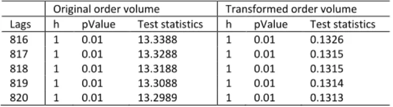
Original order volume Transformed order volume Lags h pValue Test statistics h pValue Test statistics 816 1 0.01 13.3388 1 0.01 0.1326 817 1 0.01 13.3288 1 0.01 0.1315 818 1 0.01 13.3188 1 0.01 0.1315 819 1 0.01 13.3088 1 0.01 0.1314 820 1 0.01 13.2989 1 0.01 0.1313

Table 4 KPSS test of original and transformed order lifecycles on MSFT stock (24 Jan 2013)

Original lifecycle Transformed lifecycle Lags h pValue Test Statistics h pValue Test Statistics 816 1 0.01 18.3574 1 0.01 0.1651 817 1 0.01 16.6305 1 0.01 0.1524 818 1 0.01 15.3079 1 0.01 0.1416 819 1 0.01 14.0220 1 0.01 0.1321 820 1 0.01 13.5401 1 0.01 0.1239

In the example in Table 2Table 4, the tests on the transformed ask and bid prices fail to reject the hypothesis of

stationarity, while other tests all reject it. However, in the rejected tests, the test statistics of the transformed data are all significantly smaller than that of the original data. The test statistic in KPSS, defined as , where is the Newey-West estimate of the long-run variance, , and values are the residuals, is designed for the null hypothesis of stationarity and shall be close to zero under stationary null (Kwiatkowski, Phillips, Schmidt, & Shin, 1992). This indicates that the level of dispersion in the transformed data is far lower than that found in the original data, which suggests that the non-stationarity of transformed data tends to be reduced. Similar results are also observed in Google, Apple and Amazon stock data on 18 Oct 2013. Therefore, we use the proposed transformation as a feature extraction method to reduce the non-stationary nature of the original data, and the detection models are trained on the transformed vector .

4.2

Disruptive trading detection

As discussed in Section 3.1, traders can use either single or multiple disruptive orders to induce abnormal market impacts and make a profit. Disruptive orders show anomalous behaviours to legitimate trading actions on the order book, as shown in Figure 1. We propose an anomaly detection algorithm-based model for detecting both the single-

ACCEPTED MANUSCRIPT

19 and multiple-order disruptive trading actions. An anomaly detection algorithm is used due to the following two

reasons:

1) Among the mass of normal trading data generated everyday around the world, only a small percentage is related to disruptive trading activities. Without effective monitoring mechanisms, those disruptive trading cases are very costly to find via the manual checking of financial experts. At the same time, regulatory rules usually prohibit the disclosure of those illegitimate trading behaviours.

2) Furthermore, disruptive trading tactics are also evolving over time. The collected disruptive cases only reflect “old” manipulation types, which might not contain the same features as the evolved manipulations. Modelling based on those data cannot achieve a good detection rate.

Disruptive order detection can be considered as an anomaly detection problem, which is the identification of new or unknown data patterns not exposed during the model training process. According to the discussion in Section 3, detecting disruptive trading behaviours requires monitoring each single order and multiple orders as a sequence; therefore, we propose an anomaly detection-based hybrid model composed of two components, the monitoring of single and multiple orders, for complete detection of all types of disruptive trading behaviours. The detection flow employing the proposed hybrid model is described in Algorithm 1 and illustrated in Figure 5, where the “Single Order Detection” and “Order Sequence Detection” modules represent two components of the hybrid model, and other modules represent the input order stream handlers for the models. The original order stream is transformed into the impulse vector , and each single vector is monitored through the module “Single Order Detection” for single-order disruptive trading behaviours (Steps 1-3 in Algorithm 1); afterwards, the vector sequence constructed in the sliding window is further monitored by “Order Sequence Detection” for multi-order disruptive behaviours (Steps 4-5 in Algorithm 1). The two components of the hybrid model are trained separately by the historical data before commencing the detection. The design details of the hybrid model are discussed in the following sections.

ACCEPTED MANUSCRIPT

20

Limit Order Stream

Sliding Window, length T

Order Transform Single Order Detection Construct Sequence Order Sequence Detection Single-Order Disruptive Trading Alert Not Disruptive Disruptive

+

Single Disruptive Order Detection

Multiple Disruptive Order Detection

Not Disruptive Multi-Order Disruptive Trading Alert Original limit orders Construct vector i i  i  i  Adaptive Mechanism Adaptive Mechanism

Figure 5 the detection flow employing the proposed hybrid model for single- and multiple-order disruptive trading behaviours Algorithm 1 Detection flow of the proposed hybrid detection model in Figure 5

Step 1: For any equity, collect all submitted orders and construct the Limit Order Stream for this equity; Step 2: Transform the original order stream through the “Order Transform” module based on equation 1-6;

Construct the transformed vector ;

Step 3: Detect each vector through the “Single Order Detection” module for single-order disruptive trading behaviour; if detected, trigger the alert; Step 4: If not detected, select a sliding window length and construct a sequence of within the sliding window;

Step 5: Detect the constructed sequence through the “Order Sequence Detection” module; if detected, trigger the alert; if not, update the sliding window with the newest transformed order.

4.2.1

Single-order disruptive trading detection

A single disruptive order is designed by traders by tuning the quoted price, volume and life cycle of the submitted limit orders, which are usually designed and placed to the market individually with no sequential relations. To detect such types of disruptive orders, the proposed model is to monitor each trading order individually and compare it with historical legitimate trading behaviours to recognise manipulative patterns. If represented through the transformed impulse , as shown in Figure 3, the disruptive orders are against most of the legitimate trading behaviours. In an anomaly detection area, one-class support vector machine (OCSVM) is one of the most ideal algorithms to provide a direct description of the boundary (the support vectors) between anomalies and normalities (Schölkopf, Platt, Shawe-Taylor, Smola, & Williamson, 2001 ) (Hayton, et al., 2006). OCSVM applied to single-disruptive-order detection provides a measure of disruptive orders by learning a representation of normal and legitimate trading orders. Therefore, in this paper, OCSVM is proposed as the “Single Order Detection” module in Figure 5. As discussed in Algorithm 1, the original limit orders are transformed and then used to construct the impulse vector

ACCEPTED MANUSCRIPT

21 OCSVM is applied as disruptive order detection, it considers each vector as a single object. Therefore, the “Single Order Detection” module can only monitor the disruptive trading behaviours of a single order.

4.2.2

Multi-order disruptive trading detection

Disruptive trading can also be carried out by submitting multiple limit orders to the market as a sequence with no intention of execution. Such order sequences quick sweeting the market induces the market impact by successively aggressive quotes or volumes. The grey points in Figure 3(b-c) show the behaviours of such a strategy in transformed formats. Detecting such behaviours requires recognising the temporal change among disruptive orders in the sequence. To further identify the trading intentions, we need to determine the strategies capable of generating the observed temporal changes, as well as the probability of the occurrence of the observed temporal changes. A hidden Markov Model (HMM) containing two sets of states, observable feature states and hidden mixture component states, can be used to model such cases. These HMM contents are modelled on a standard Markov process on the assumption that they depend solely on previous states. Usually, the application of an HMM can be categorised as belonging to one of two classes; the first is signature modelling, where the detection model is learned from the activities to be recognised, and the activities matching the model are reported as detection outcomes. Examples of this include the coupled

behaviour detection in (Cao, Ou, & Yu, 2012), the industry process monitoring in (Wang, Mehrabi, & Kannatey-Asibu, 2002) and (Bruce, 2009), the intrusion detected in (Yeung & Ding, 2003) and the video surveillance in (Guo, Miao, Zhang, Shen, & Wang, 2012). The other category of HMM application is anomaly detection, whereby a model of normality is learned solely from the normal activity, and cases tested against the model, with a pre-determined

threshold, are declared to be anomalies (Yeung & Ding, 2003). In such cases, it is very important that the hidden states be identified and assigned, thereby fulfilling the Markov assumption and allowing the parameter matrices to generate different observed outputs.

As discussed in the previous section, the detection of disruptive trading behaviours intended to mislead market prices can be framed as an anomaly detection problem, which is to identify new or unknown patterns that have not previously been clarified during the detection model training process (disruptive trading data has not been disclosed in accordance with industry regulations). Utilizing the anomaly detection approach requires that the normal patterns be modelled and

ACCEPTED MANUSCRIPT

22 that an “alarm” be triggered when market activity deviates from those normal patterns. To do this, an improved and adapted HMM with anomaly states has been developed and is presented in the following sections.

4.2.2.1

The multi-variable Gaussian mixture model

Financial data are generally considered to be inherently non-stationary, and so it is accepted that the statistical properties of such data, for example, the mean and variance, vary over time. These variations result from a range of factors, including business and economic cycles and demand/supply microstructures. That makes it particularly interesting when unusual activities are associated with a lack of stationarity in the extracted features, i.e., when the distribution of those extracted features is altered during its existence. This variation can be observed as an outcome of various irregular trading activities; thus, the detection model must have the capacity not only to capture the

distributions of the extracted features but also to track shifts in them. Therefore, distribution, followed by sequential data modelling methods, is suggested for the detection model in this section.

An established method for modelling the probability density function (PDF) of a variable is to approximate its (unknown) density using a Gaussian mixture model (GMM) (Bishop, 2006). A GMM is a weighted sum of M-component Gaussian densities as , where is a D−dimensional continuous-valued data vector, , , are mixture weights, and , , are component Gaussian densities, wherein

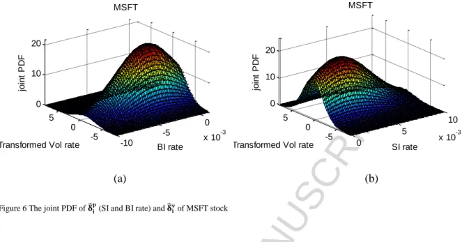
and are the mean and covariance matrix for each component, respectively. Each component density is a D−variate Gaussian function. To capture the temporal changes of the multi-order disruptive trading features, we construct and calculate two intuitive features that are associated with the patterns of multi-order trading behaviours; this is defined as the change rate of and with respect to the lifecycle of the order: , where and . In the interest of detecting unusual distributions of and , the joint PDF of and are modelled using GMM. Figure shows an example of the joint PDF of and of MSFT stock. The joint PDF of buy (BI) and sell (SI) orders are constructed as in Figure (a) and (b), respectively, and show distinct distributions, which are also observed in Figure 4 where the buy and sell impulses are distributed apart in separated sides along the zero point. Therefore, the buy and sell behaviours are modelled separately.

ACCEPTED MANUSCRIPT

23

(a) (b)

Figure 6 The joint PDF of (SI and BI rate) and of MSFT stock

We also illustrate the reported disruptive trading cases of MSFT stock (represented in Figure 3) in Figure 6(a, c), and on the contours of the joint PDFs in Figure 8. The disruptive trading cases (red circles in Figure 6(a, c)) lie on the edge areas of the two distributions. However, among the mass of normal trading data generated everyday around the world, only a small percentage is related to disruptive trading activities. The reported cases are even fewer due to the

regulatory rules discussed in Section 4.2. To effectively overcome the imbalanced dataset of disruptive and legitimate trading cases and identify the distribution of the disruptive trading cases, we follow the traditional hybrid SMOTE-RUS approach that combines the widely used over-sampling algorithm SMOTE (Chawla, Bowyer, Hall, &

Kegelmeyer, 2002) and under-sampling algorithm RUS together (Ng, Hu, Yeung, Yin, & Roli, 2014). To achieve a reasonably balanced ratio in the dataset, the SMOTE algorithm is slightly revised by taking each minority class example and randomly generating synthetic examples along the line segments joining all other examples in the minority class. Each of the synthetic examples is generated following the traditional SMOTE approach. Figure 6 illustrates an example of the SMOTE-RUS approach on the MSFT stock dataset in a short time interval. 30 reported disruptive examples are represented as red circles in Figure 6 as 15 disruptive sell orders in (a) and 15 disruptive buy orders in (c) with 20000 normal examples. If the expected ratio is 1:1 on both the buy and sell sides, the normal examples can be under-sampled by 10% to , and the disruptive examples can be over-sampled by

taking to contain examples as in the illustration in Figure 6(b, d). Therefore, the hybrid approach generates a dataset with a ratio of minority and majority. Training a model on

-10 -5 0 x 10-3 -5 0 5 0 10 20 BI rate MSFT

Transformed Vol rate

jo in t P D F 0 5 10 x 10-3 -5 0 5 0 10 20 SI rate MSFT

Transformed Vol rate

jo in t P D F

ACCEPTED MANUSCRIPT

24 such a balanced dataset would obviously result in unbiased performance. In addition, the joint PDF of the balanced data illustrated in Figure 6 (b) and (d) are then constructed by GMM, as shown in Figure 6.

(a) (b)

(c) (d)

Figure 6 (a) buy side MSFT trading data from 9:00-12:00 am on 24 Jan 2013 with a 15:20000 ratio of disruptive (red circles) and normal (blue dots) trading data; (b) data examples generated by the hybrid SMOTE-RUS approach on the data in (a) with a 0.95:1 ratio of disruptive (red circles) and normal examples; (c) sell side MSFT trading data from 9:00-12:00 am on 24 Jan 2013 with a 15:20000 ratio of disruptive (red) and normal (blue dots) trading data; (d) data examples generated by the hybrid SMOTE-RUS approach with a 0.96:1 ratio of minority (red circles and red dots) and majority (blue dots)

(a) (b)

Figure 7 The contour of the joint PDF of the under-sampled normal trading data (in Figure 6) and the over-sampled disruptive trading cases by the SMOTE-RUS approach

4.2.2.2

HMM-based model

As shown in Figure 7, we construct the joint PDF of normal and disruptive trading behaviours separately using GMM, and the two PDFs are represented as (normal) and (disruptive). We setup the probability thresholds for

ACCEPTED MANUSCRIPT

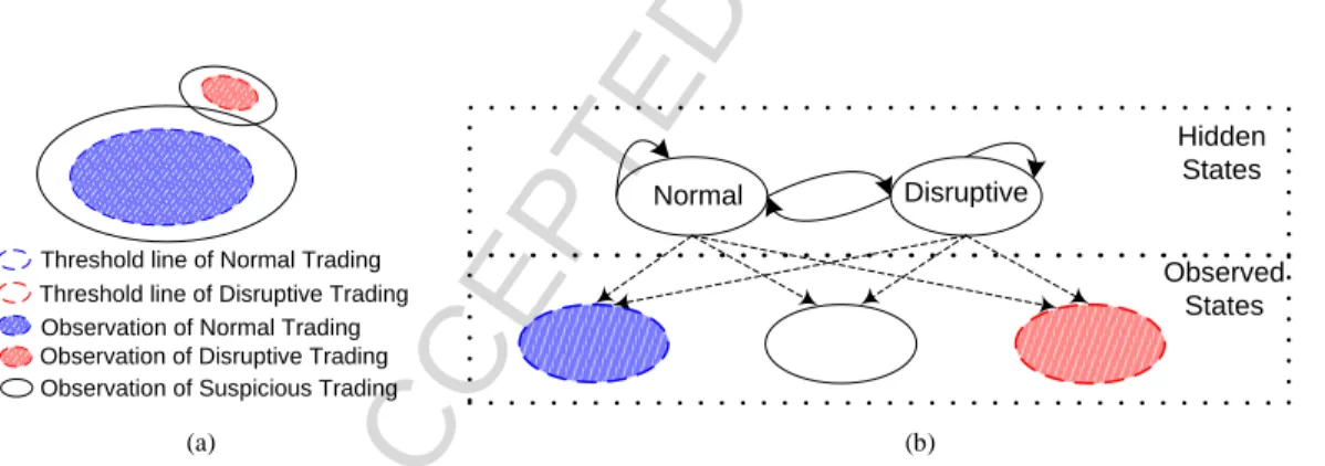
25 (OCSVM) (Schölkopf, Platt, Shawe-Taylor, Smola, & Williamson, 2001 ), where the threshold is generally set to include most (for example, 99%) but not all training data to avoid a high misdetection rate. For , the probability threshold is set as 99% of the lowest cumulative probability of normal trading examples. In other words, the data are accepted as normal when . Similarly, for , the threshold is set as 99% of the lowest cumulative probability of disruptive trading examples. The 1% outlying values are not simply taken as abnormalities but are used to generate the states for the HMM. By this, two thresholds provide a simplified and joint state view of the two sequential time series and . Thus, the two joint PDFs can be divided into three states, as in the example shown in Figure 8(a), one of which (blue area, ) corresponds to the normal trading behaviours, another (red area, ) is disruptive trading behaviours, and the remaining area (white,

_{or ) is correlated with the suspicious trading behaviours, which is neither}

normal nor disruptive by itself. Because a single disruptive trade may afterwards imply disruptive behaviours, the determination of multi-order disruptive trading depends on other behaviours in a sequence.

Observation of Disruptive Trading Observation of Suspicious Trading Observation of Normal Trading Threshold line of Normal Trading Threshold line of Disruptive Trading

Disruptive Normal Hidden States Observed States (a) (b)

Figure 8 (a) Example of states of observed trading behaviours; (b) Structure of the designed Hidden Markov Model with Disruptive states

To determine the legitimacy of a sequence of trading behaviours, we designate two hidden states representing latent normal and disruptive intentions. Therefore, the hidden Markov model, HMM, is designed as in Figure 8(b). The state that satisfies (the blue area of normality in Figure 8(b)) is considered to be a completely normal hidden state, while the state that satisfies (the red area of disruptiveness in Figure 8(b)) is thus defined as a hidden disruptive state, and the other states satisfy either or (white suspicious but not deterministic area in Figure 8(b)). This HMM design presents an efficient means of

modelling the limit order streams, and in this context, the observed temporal dynamics of the trading behaviours are simply represented as the hidden state transitions as shown in Figure 8(b). The fundamental property of this design utilizes the inference features of HMM, which could answer two key questions: 1) what is the most likely sequence of

ACCEPTED MANUSCRIPT

26 hidden states to generate the observed sequence (what is the latent intention given a certain observed trading sequence), and 2) what is the probability of an observed sequence (how likely are we to observe a specific trading sequence)? HMM provides answers to the two questions by determining the sequence of hidden states most likely generating the observations sequences and the occurrence probability of the observed sequence based on the transition and emission probability matrix constructed during the training process. Those answers can be used as a measure of disruptive trading behaviours.

4.2.3

Adaptive mechanism

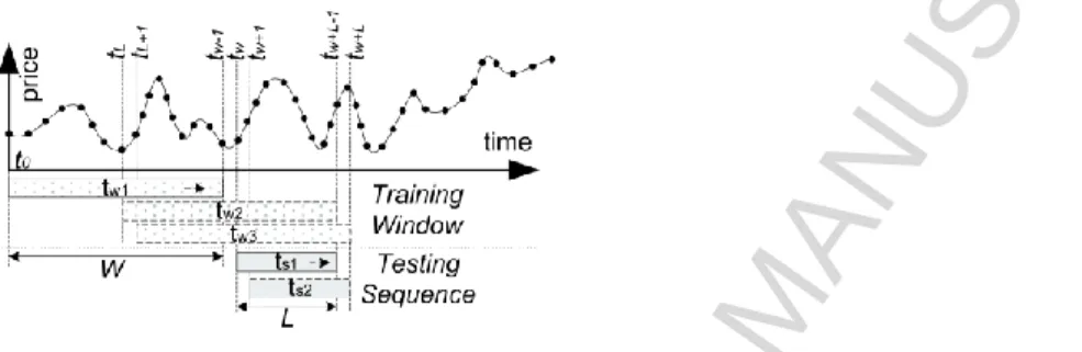
The financial time series is non-stationary. Although the non-stationary nature of the transformed impulse is reduced based on the test results in Table 2-Table 4, the mean and variance of the constructed joint PDFs may be subject to variation over time. To mitigate the non-stationarity, the proposed detection model is augmented with an adaptive mechanism. The detection models, OCSVM for single-order and HMM for multi-order disruptive behaviours, are trained using data in a sliding window of length . During the process of disruptive trading behaviour detection, the window slides forward and maintains the closest data points, and the OCSVM and HMM are updated if any meaningful differences between the data points in the current sliding window and prior training data are found. The Mann–Whitney U test (MWW) (Fay & Proschan, 2010), a nonparametric test of the null hypothesis that two samples come from the same population, is used to identify a deviation between the two data sequences. MWW can be applied on an unknown distribution, contrary to the t-test, which can only be applied on normal distributions, and it is nearly as efficient as the t-test on normal distributions (Fay & Proschan, 2010). The MWW is designed as an independent module and is used as a post-processing block of the detection model to identify the significant differences between the updated data sequence in the sliding window and the prior training data sequence. Figure 9 describes the proposed adaptive mechanism of the proposed model for detecting disruptive trading behaviours. At first, the OCSVM and HMM are trained separately by differently calculated features from w data points in the training window, , where and are the starting and ending time points, respectively. OCSVM uses

, and HMM uses . For OCSVM, the first testing sample is the trading

ACCEPTED MANUSCRIPT

27 first test case; if this is assessed as normal, the training sliding window is slid to for significant difference testing by MWW. If a significant change is detected, both the OCSVM and the HMM model are re-trained by the data in , and if not, the test case for OCSVM is updated as the trading order and the test

sequence for the HMM is then updated into the window . The length of the testing sequence in

Figure 5 is then set equal to the length of and . The training window in our proposed mechanism is set to a single

day because the disruptive trading actions are usually completed within a short time period as intraday activities, and setting the window to one single day is enough to cover the data features for training the detection model.

Figure 9 The training and testing mechanism of the multi-order disruptive trading behaviour detection model

4.2.4

The detection algorithm

As per the discussion in Section 4.2, Algorithm 1 provides a complete structure of the workflow of the detection algorithm. The steps of the “Single Order Detection” and “Order Sequence Detection” modules together with the “Adaptive Mechanism” module are summarised in Algorithm 2 and Algorithm 3, respectively, below. Therefore, the disruptive trading behaviour hybrid detection model is constructed by Algorithm 1-Algorithm 3.

Algorithm 2 Workflow of the proposed “Single Order Detection” and “Adaptive Mechanism” module in Figure 5

Step 1: Select a historical date and construct the training dataset of the transformed vector

;

Step 2: Train the OCSVM using the constructed training dataset;

Step 3: Detect the most updated incoming vector using the trained OCSVM;

Step 4: If OCSVM triggers a disruptive trading alert, the most updated vector is stored in the disruptive trading dataset;

Step 5: If no disruptive trading alert is triggered, the training dataset is slid forward to include the most updated vector and is fed into the adaptive mechanism module for a model update check. If a model update is needed, the algorithm flow goes to Step 2.

Step 6: If a model update is not needed, the algorithm flow goes to Step 3.

Algorithm 3 Workflow of the proposed “Order Sequence Detection” and “Adaptive Mechanism” module in Figure 5

Step 1: Select a historical date and construct the training dataset of the transformed vector ; Step 2: _{Calculate and construct the training dataset of ;}

Step 3: Collect all known disruptive trading records on the selected financial instrument and construct the dataset of the transformed disruptive vector ;

ACCEPTED MANUSCRIPT

28 Step 4: _{Calculate and construct the training dataset of}

;

Step 5: Apply Algorithm 2 on the dataset of and construct the over-sampled dataset

of ;

Step 6: Calculate the joint PDF of vectors and using GMM;

Set the corresponding thresholds for two joint PDFs;

Construct the hidden and observed states according to the discussion in Section 4.2.2.2 and the illustrations in Figure 7 and Figure 8;

Step 7: Train the HMM using the constructed vectors and states;

Step 8: For a constructed testing sequence , detect disruptive behaviours via the trained HMM model;

Step 9: If HMM triggers a disruptive trading alert, the corresponding vectors are stored in the disruptive trading dataset; the algorithm flow goes to Step 5;

Step 10: If no alert is triggered, the training dataset is slid forward to include the most updated vector and is fed into the adaptive mechanism module for a model update check. If a model update is needed, the algorithm flow goes to Step 2;

Step 11: If a model update is not needed, the testing sequence is slid forward to include the most updated vector, and the algorithm flow goes to Step 8;

4.3

Experimental evaluation

A large amount of labelled examples of both normal and disruptive trading data are commonly used in evaluating a detection model. However, given the lack of genuine market data of disruptive trading behaviour, a slightly adapted approach is taken in this case. To evaluate the proposed detection model, the characteristics of the disruptive trading behaviours have been studied, synthetically generated, and then injected into the financial time-series data. Meanwhile, statistical features such as mean, variance and volatility are all maintained.

4.3.1

The experimental setup

In this paper, experimental evaluation is conducted using genuine market data from four representative stocks: Google, Microsoft, Intel and Apple from the NASDAQ. These datasets were chosen because they have relatively high trading volumes and price volatility, which are elements likely to induce manipulation across exchanges (Cumming, Zhan, & Aitken, 2013); thus, they are at greater risk of manipulation than many others. The dataset covers tick trading data over the entire year of 2013, and the data in every trading day comprises approximately 400,000 samples for each stock. The dataset for each selected stock contains more than 10 Gigabytes of data. All of the datasets have been examined by the authors’ expert financial partners to ensure that none of them are related to any cases of disruptive behaviour that have been reported to the regulatory authorities. The experiments are designed by reproducing the reported examples and then injecting them into the dataset of corresponding stocks, which means that the test data becomes a mix of both normal and anomalous patterns. The trained models are then applied to that mixed data to identify patterns associated

ACCEPTED MANUSCRIPT

29 with disruptive behaviours. This approach is of acknowledged value to the industry, particularly given the huge

expense involved in isolating genuine trading cases. The experiments are therefore designed in three groups:

Group 1: The single-order disruptive trading behaviour in Figure 1 is reproduced in the datasets of the selected stocks using original characteristics discussed in Section 3.1. Five hundred examples are reproduced and injected in four datasets.

Group 2: Five hundred examples of the multi-order disruptive trading behaviour in Figure 2 are reproduced and injected in four datasets.

Group 3: Five hundred examples of mixed disruptive behaviours (half by single-order and half by multi-order) are reproduced and injected in four datasets.

The adaptive mechanism has a sliding window set to a length of one day since the disruptive trading behaviours usually target intra-day transactions to make a profit. Therefore, the genuine market trading data from 2 Jan 2013, the first trading day of 2013, was collected as the initial training dataset. The 400,000-point training dataset is partitioned into five equal-sized subsets. The cross-validation is then repeated five times. Each time, one single subset is retained as the testing dataset, and the remaining four subsets are used as the training data. The five results from the cross-validation are then averaged to produce a stable trained model. The experiments are designed as an on-line real-time detection scheme. After the model is initially trained, the data are fed into the model sequentially as an order time series. The model detects and reports the disruptive behaviour according to the detection flow illustrated in Figure 5 and is re-trained and updated according to the calculations of the adaptive mechanism represented in Figure 9.

As shown in the literature review of this paper, some generic computational models have already been applied to the problem of detecting similar disruptive patterns; these include k-nearest neighbour (kNN), Gaussian MM and logistic regression (LR) approaches (Aitken, Harris, & Ji, 2009) (Öğüt, Doğana, & Aktaş, 2009) (Diaz, Theodoulidis, & Sampaio, 2011). The three popular computational models are selected as benchmarks for evaluating the proposed model and are applied on the data sequence in the same scheme as the proposed model. The three benchmark models are fine-tuned through the application of five-fold cross-validation on each different dataset to ensure the stability and

ACCEPTED MANUSCRIPT

30 quality of the results. The basic accuracy measures, precision, recall, F measure and G measure, as well as the ROC curve and AUC, are used as performance measures for the evaluation.

4.3.2

Results of experimental assessment

The precision, recall, F and G measure for the four models on four different datasets are represented in Table 5-Table 7. From all of the experiments in the three groups, we can observe that the proposed hybrid model achieved stable and constantly better performances then all other benchmark models in terms of recall, precision, F and G measures. Table 5 Recall, Precision, F measure and G score of the Group 1 experimental results for four models on four datasets

Recall Precision F measure G score

APPA Hybrid 0.9717 0.9749 0.9733 0.9733 kNN 0.8902 0.9528 0.9204 0.9210 GMM 0.8221 0.9336 0.8743 0.8761 LR 0.8210 0.8938 0.8559 0.8567 GOOG Hybrid 0.9801 0.9699 0.9750 0.9750 kNN 0.9046 0.9494 0.9264 0.9267 GMM 0.9020 0.9505 0.9256 0.9259 LR 0.8020 0.9225 0.8580 0.8601 INTL Hybrid 0.9648 0.9847 0.9746 0.9747 kNN 0.8937 0.9546 0.9231 0.9236 GMM 0.8639 0.9514 0.9055 0.9066 LR 0.8490 0.9402 0.8923 0.8934 MSFT Hybrid 0.9678 0.9742 0.9710 0.9710 kNN 0.8968 0.9672 0.9307 0.9314 GMM 0.8833 0.9321 0.9070 0.9074 LR 0.8200 0.9100 0.8626 0.8638

Table 6 Recall, Precision, F measure and G score of the Group 2 experimental results for four models on four datasets

Recall Precision F measure G score

APPA Hybrid 0.9468 0.9682 0.9574 0.9574 kNN 0.8510 0.9327 0.8900 0.8909 GMM 0.8663 0.9448 0.9038 0.9047 LR 0.8700 0.9275 0.8978 0.8983 GOOG Hybrid 0.9705 0.9678 0.9692 0.9692 kNN 0.8077 0.9394 0.8685 0.8710 GMM 0.8802 0.9468 0.9123 0.9129 LR 0.8700 0.9242 0.8963 0.8967 INTL Hybrid 0.9725 0.9805 0.9765 0.9765 kNN 0.8299 0.9425 0.8826 0.8844 GMM 0.8903 0.9473 0.9179 0.9184 LR 0.8702 0.9381 0.9029 0.9035 MSFT Hybrid 0.9883 0.9832 0.9857 0.9858 kNN 0.8610 0.9561 0.9061 0.9073 GMM 0.8737 0.9468 0.9088 0.9095 LR 0.8490 0.9003 0.8739 0.8743

Table 7 Recall, Precision, F measure and G score of the Group 3 experimental results for four models on four datasets

Recall Precision F measure G score

APPA

Hybrid 0.9203 0.9809 0.9497 0.9501

kNN 0.8578 0.9570 0.9047 0.9061 GMM 0.8357 0.9339 0.8821 0.8834