Automated, Efficient, and Practical Extreme Value Analysis with Environmental Applications

(1)

Doctoral Dissertations University of Connecticut Graduate School

9-16-2016

Automated, Efficient, and Practical Extreme Value

Analysis with Environmental Applications

Brian Bader

[email protected]

Follow this and additional works at:https://opencommons.uconn.edu/dissertations

Recommended Citation

Bader, Brian, "Automated, Efficient, and Practical Extreme Value Analysis with Environmental Applications" (2016).Doctoral Dissertations. 1261.

(2)

Extreme Value Analysis with

Environmental Applications

Brian M. Bader, Ph.D. University of Connecticut, 2016

ABSTRACT

Although the fundamental probabilistic theory of extremes has been well developed, there are many practical considerations that must be addressed in application. The contribution of this thesis is four-fold. The first concerns the choice of r in ther largest order statistics modeling of extremes. Practical concern lies in choosing the value of r; a larger value necessarily reduces variance of the estimates, however there is a trade-off in that it may also introduce bias. Current model diagnostics are somewhat restrictive, either involving prior knowledge about the domain of the distribution or using visual tools. We propose a pair of formal goodness-of-fit tests, which can be carried out in a sequential manner to select r. A recently developed adjustment for multiplicity in the ordered, sequential setting is applied to provide error control. It is shown via simulation that both tests hold their size and have adequate power to detect deviations from the null model.

(3)

approach. Existing methods for threshold selection in practice are informal as in visual diagnostics or rules of thumb, computationally expensive, or do not account for the multiple testing issue. We take a methodological approach, modifying existing goodness-of-fit tests combined with appropriate error control for multiplicity to provide an efficient, automated procedure for threshold selection in large scale problems.

The third combines a theoretical and methodological approach to improve estimation within non-stationary regional frequency models of extremal data. Two alternative methods of estimation to maximum likelihood (ML), maximum product spacing (MPS) and a hybrid L-moment / likelihood approach are incorporated in this framework. In addition to having desirable theoretical properties compared to ML, it is shown through simulation that these alternative estimators are more efficient in short record lengths.

The methodology developed is demonstrated with climate based applications. Last, an overview of computational issues for extremes is provided, along with a brief tutorial of the R packageeva, which improves the functionality of existing extreme value software, as well as contributing new implementations.

(4)

Extreme Value Analysis with

Environmental Applications

Brian M. Bader

B.A., Mathematics, Stony Brook University, NY, USA, 2009 M.A., Statistics, Columbia University, NY, USA, 2011

A Dissertation

Submitted in Partial Fulfillment of the Requirements for the Degree of

Doctor of Philosophy at the

University of Connecticut 2016

(5)

Copyright by

Brian M. Bader

(6)

APPROVAL PAGE

Doctor of Philosophy Dissertation

Automated, Efficient, and Practical Extreme Value

Analysis with Environmental Applications

Presented by

Brian M. Bader, B.A. Mathematics, M.A. Statistics

Major Advisor Jun Yan Associate Advisor Kun Chen Associate Advisor Dipak K. Dey Associate Advisor Xuebin Zhang University of Connecticut 2016

(7)

Acknowledgements

“On this life that we call home, the years go fast and the days go so slow.” — Modest Mouse

This is sound advice for anyone considering to pursue a PhD. It’s hard to believe this chapter of my life is coming to an end — the past four years have gone so fast, yet at times I thought it would never come soon enough. It has been full of ups and downs, but at the lowest of times, the only thing to do was continue on. I’ve made many new friends (who will hopefully turn into old), mentors, and gained precious knowledge that I think will benefit me throughout the rest of my life.

I’d like to thank Dr. Ming-Hui Chen for guiding me through the qualifying exam process and allowing me to thrive in the Statistical Consulting Service. I’ve gained valuable experience from participating in this group. I appreciate Dr. Dipak Dey for taking time out of his busy schedule as a dean to give me advice, recommendations, and to be on this committee. The same appreciation goes to Dr. Kun Chen for agreeing to be on my committee. Suggestions by Dr. Vartan Choulakian and Dr. Zhiyi Chi helped improve some of the methodology and data analysis in this research.

Dr. Jun Yan, my major advisor, has guided me throughout the research process and pushed me along to make sure I completed all the necessary milestones in a timely manner. I must admit that I was slightly intimidated of him at first, but I now believe

(8)

that he is most likely the best choice of advisor (for me) and I am glad things fell into place as such. He is truly a kind person and has always been understanding of any problems I have had over the past two years. Although I am not pursuing the academic route at the moment, I appreciate his enthusiastic nudge for me to go in that direction. Additionally, Dr. Xuebin Zhang has graciously spent his time and energy into con-versations with myself and Dr. Yan to improve our manuscripts and our knowledge of environmental extremes. Of course I am thankful of the support he and Environment and Climate Change Canada gave by funding some of this research.

The journey would not have been the same with a different cohort — I am grateful to all their support and friendship during such trying times. I have to acknowledge my family for encouraging me to follow my academic pursuits even if it meant not seeing me as often as they’d like during these four years. The same goes for all my friends back home.

Last, but not least, I wouldn’t have made it through without the full support of my wife Deirdre and two cats Eva and Cuddlemonkey (who joined our family as a result of all this). I cannot express my total love and gratitude for them in words.

This research was partially supported by an NSF grant (DMS 1521730), a Univer-sity of Connecticut Research Excellence Program grant, and Environment and Climate Change Canada.

(9)

List of Tables

2.1 Empirical size (in %) for the parametric bootstrap score test under the null distribution GEVr, with µ = 0 and σ = 1 based on 1000 samples, each with bootstrap sample sizeL= 1000. . . 33 2.2 Empirical size (in %) for multiplier bootstrap score test under the null

distribution GEVr, with µ = 0 and σ = 1. 1000 samples, each with bootstrap sample size L = 1000 were used. Although not shown, the empirical size for r= 1 and ξ =−0.25 becomes acceptable when sample size is 1000. . . 34 2.3 Empirical size (in %) for the entropy difference (ED) test under the null

distribution GEVr, with µ= 0 and σ= 1 based on 10,000 samples. . . . 35 2.4 Empirical rejection rate (in %) of the multiplier score test and the ED

test in the first data generating scheme in Section 2.5.2 from 1000 replicates. 37 2.5 Empirical rejection rate (in %) of the multiplier score test and the ED test

(14)

2.6 Percentage of choice of r using the ForwardStop and StrongStop rules at various significance levels or FDRs, under ED, parametric bootstrap (PB) score, and multiplier bootstrap (MB) score tests, with n = 100 and ξ = 0.25 for the simulation setting described in Section 2.6. Correct choice is r= 4. . . 45 3.1 Empirical rejection rates of four goodness-of-fit tests for GPD under

var-ious data generation schemes described in Section 3.3.4 with nominal size 0.05. GPDMix(a, b) refers to a 50/50 mixture of GPD(1, a) and GPD(1, b). . . 70 4.1 Failure rate (%) in optimization for the three estimation methods in the

combined 12 settings of number of sites, observations, and dependence levels within each spatial dependence structure (SC, SM, and GC) out of 10,000 replicates. The setup is described in detail in Section 4.4. . . 103

(15)

List of Figures

1.1 The density function of the Generalized Extreme Value distribution for shape parameter values of −0.5, 0, and 0.5 with location and scale pa-rameters fixed at zero and one, respectively. . . 5 1.2 A comparison of extremes selected via the peaks over threshold (left)

versus block maxima approach for example time series data. . . 6 1.3 Mean Residual Life plot of Fort Collins daily precipitation data found in

R package extRemes. . . 13 1.4 Threshold stability plot for the shape parameter of the Fort Collins daily

precipitation data found in R package extRemes. . . 14 1.5 Hill plot of the Fort Collins daily precipitation data found in R package

extRemes. . . 14 2.1 Comparisons of the empirical vs. χ2(3) distribution (solid curve) based on

5000 replicates of the score test statistic under the null GEVrdistribution. The number of blocks used is n = 5000 with parameters µ = 0, σ = 1, and ξ∈(−0.25,0.25). . . 26

(16)

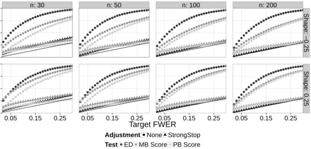
2.2 Observed FWER for the ED, parametric bootstrap (PB) score, and multi-plier bootstrap (MB) score tests (using No Adjustment and StrongStop) versus expected FWER at various nominal levels. The 45 degree line indicates agreement between the observed and expected rates under H0. . 42

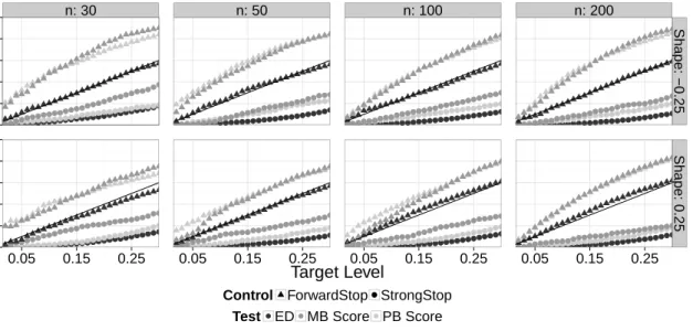
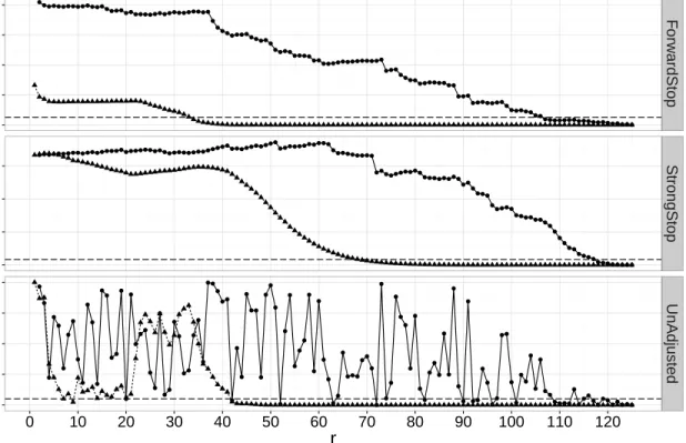
2.3 Observed FDR (from ForwardStop) and observed FWER (from StrongStop) versus expected FDR and FWER, respectively, at various nominal levels. This is for the simulation setting described in Section 2.6, using the ED, parametric bootstrap (PB) score, and multiplier bootstrap (MB) score tests. The 45 degree line indicates agreement between the observed and expected rates. . . 43 2.4 Adjusted p-values using ForwardStop, StrongStop, and raw (unadjusted)

p-values for the ED and PB Score tests applied to the Lowestoft sea level data. The horizontal dashed line represents the 0.05 possible cutoff value. 48 2.5 Location, scale, and shape parameter estimates, with 95% delta

confi-dence intervals for r = 1, . . . ,40 for the Lowestoft sea level data. Also included are the estimates and 95% profile likelihood confidence intervals for the 50, 100, and 200 year return levels. The vertical dashed line repre-sents the recommended cutoff value ofr from the analysis in Section 2.7.1. 49

(17)

2.6 Adjusted p-values using ForwardStop, StrongStop, and raw (unadjusted) p-values for the ED and PB Score tests applied to the Atlantic City pre-cipitation data. The horizontal dashed line represents the 0.05 possible cutoff value. . . 51 2.7 Location, scale, and shape parameter estimates, with 95% delta

confi-dence intervals for r = 1 through r = 10 for the Atlantic City precipi-tation data. Also included are the estimates and 95% profile likelihood confidence intervals for the 50, 100, and 200 year return levels. The ver-tical dashed line represents the recommended cutoff value of r from the analysis in Section 2.7.2. . . 52 3.1 Observed FWER for the Anderson–Darling test (using StrongStop and

no adjustment) versus expected FWER at various nominal levels under the null GPD at ten thresholds for 10,000 replicates in each setting as described in Section 3.4. The 45 degree line indicates agreement between the observed and expected rates under H0. . . 72 3.2 Plot of the (scaled) density of the mixture distribution used to generate

misspecification ofH0 for the simulation in Section 3.4. The vertical line

(18)

3.3 Frequency distribution (out of 1000 simulations) of the number of rejec-tions for the Anderson–Darling test and various stopping rules (Forward-Stop, Strong(Forward-Stop, and no adjustment), at the 5% nominal level, for the misspecified distribution sequential simulation setting described in Sec-tion 3.4. 50 thresholds are tested, with the 34th being the true threshold. 75 3.4 Observed FDR (using ForwardStop) and observed FWER (using StrongStop)

versus expected FDR and FWER respectively using the Anderson–Darling test, at various nominal levels. This is for the sequential simulation set-ting under misspecification described in Section 3.4. The 45 degree line indicates agreement between the observed and expected rates. . . 76 3.5 Average performance comparison of the three stopping rules in the

sim-ulation study under misspecification in Section 3.4, using the Anderson– Darling test for various parameters. Shown are the relative frequencies of the average value of each metric (bias, squared error, and coverage) for each stopping rule and parameter of interest. For each parameter of interest and metric, the sum of average values for the three stopping rules equates to 100%. RL refers to return level. . . 77 3.6 Distribution of chosen percentiles (thresholds) for the 720 western US

coastal sites, as selected by each stopping rule. Note that this does not include sites where all thresholds were rejected by the stopping rule. . . . 81

(19)

3.7 Map of US west coast sites for which all thresholds were rejected (black / circle) and for which a threshold was selected (grey / triangle), by stopping rule. . . 82 3.8 Comparison of return level estimates (50, 100, 250, 500 year) based on the

chosen threshold for ForwardStop vs. StrongStop for the US west coast sites. The 45 degree line indicates agreement between the two estimates. This is only for the sites in which both stopping rules did not reject all thresholds. . . 83 3.9 Map of US west coast sites with 50, 100, and 250 year return level

es-timates for the threshold chosen using ForwardStop and the Anderson– Darling test. This is only for the sites in which a threshold was selected. 84 4.1 Schlather model root mean squared error of the parameters for each

es-timation method, from 1000 replicates of each setting discussed in Sec-tion 4.4. W, M, S refers to weak, medium, and strong dependence, with

m being the number of sites and n, the number of observations within each site. . . 104 4.2 Smith model root mean squared error of the parameters for each

estima-tion method, from 1000 replicates of each setting discussed in Secestima-tion 4.4. W, M, S refers to weak, medium, and strong dependence, with m being the number of sites andn, the number of observations within each site. . 105

(20)

4.3 Gaussian copula model root mean squared error of the parameters for each estimation method, from 1000 replicates of each setting discussed in Section 4.4. W, M, S refers to weak, medium, and strong dependence, withmbeing the number of sites andn, the number of observations within each site. . . 106 4.4 Locations of the 27 California sites used in the non-stationary regional

frequency analysis of annual daily maximum winter precipitation events. 108 4.5 Scatterplot of Spearman correlations by euclidean distance between each

pair of the 27 California sites used in the non-stationary regional frequency analysis of annual daily maximum winter precipitation events. . . 109 4.6 Estimates and 95% semi-parametric bootstrap confidence intervals of the

location parameter covariates (postive and negative SOI piecewise terms), proportionality, and shape parameters for the three methods of estima-tion in the non-staestima-tionary RFA of the 27 California site annual winter maximum precipitation events. . . 110 4.7 Estimates and 95% semi-parametric bootstrap confidence intervals of the

marginal site-specific location means for the three estimation methods in the non-stationary RFA of the 27 California site annual winter maximum precipitation events. . . 111

(21)

4.8 Estimates and 95% semi-parametric bootstrap confidence intervals of the shape parameter by the three estimation methods, for the full 53 year and 18 year subset sample of California annual winter precipitation extremes. The horizontal dashed line corresponds to the shape parameter estimate of each method for the subset sample. . . 112 4.9 Left: 50 year return level estimates (using MPS) at the 27 sites,

condi-tioned on the mean sample SOI value (−0.40). Right: Estimated percent increase in magnitude of the 50 year event at the sample minimum SOI (−28.30) versus the mean SOI value. . . 113 5.1 Plot of GEV cumulative distribution function with x = 1, µ = 0 and

σ = 1, with ξ ranging from −0.0001 to 0.0001 on the cubic scale. The naive implementation is represented by the solid red line, with the imple-mentation in R package evaas the dashed blue line. . . 121 5.2 Estimates and 95% profile likelihood confidence intervals for the 250 year

return level of the LoweStoft sea level dataset, for r= 1 through r= 10. 123 5.3 Estimates and 95% delta method confidence intervals for the 250 year

(22)

5.4 Plot of the largest order statistic (block maxima) from a GEV10

distri-bution with shape parameter parameter ξ = 0. The location and scale have an intercept of 100 and 1, with positive trends of 0.02 and 0.01, respectively. The indices (1 to 100) are used as the corresponding trend coefficients. . . 126

(23)

Chapter 1

Introduction

1.1

Overview of Extreme Value Analysis

Both statistical modeling and theoretical results of extremes remain a subject of active research. Extreme value theory provides a solid statistical framework to handle atypical, or heavy-tailed phenomena. There are many important applications that require mod-eling of extreme events. In hydrology, a government or developer may want an estimate of the maximum flood event that is expected to occur every 100 years, say, in order to determine the needs of a structure. In climatology, extreme value theory is used to determine if the magnitude of extremal events are time-dependent or not. Similarly, in finance, market risk assessment can be approached from an extremes standpoint. See Coles (2001); Tsay (2005); Dey and Yan (2016) for more specific examples.

Further, the study of extremes in a spatial context has been an area of interest for many researchers. In an environmental setting, one may want to know if certain geo-graphic and/or climate features have an effect on extremes of precipitation, temperature, wave height, etc. Recently, many explicit models for spatial extremes have been devel-oped. For an overview, see Davison, Padoan, Ribatet, et al. (2012). Another approach in

(24)

the same context, regional frequency anaysis (RFA), allows one to ‘trade space for time’ in order to improve the efficiency of certain parameter estimates. Roughly speaking, after estimating site-specific parameters, data are transformed onto the same scale and pooled in order to estimate the shared parameters. This approach offers two particular advantages over fully-specified multivariate models. First, only the marginal distribu-tions at each site need to be explicitly chosen – the dependence between sites can be handled by appropriate semi-parametric procedures and second, it can handle very short record lengths. See Hosking and Wallis (2005) or Wang, Yan, and Zhang (2014) for a thorough review.

A major quantity of interest in extremes is the t-period return level. This can be thought of as the maximum event that will occur on average everyt periods and can be used in various applications such as value at risk in finance and flood zone predictions. Thus, it is quite important to obtain accurate estimates of this quantity and in some cases, determine if it is non-stationary. Given some specified extremal distribution, the stationary t-period return level zt can be expressed in terms of its upper quantile

zt =Q(1−1/t) where Q(p) is the quantile function of this distribution.

Within the extreme value framework, there are several different approaches to mod-eling extremes. In the following, the various approaches will be discussed and a data

(25)

example of extreme daily precipitation events in California is used to motivate the con-tent of this thesis.

1.1.1

Block Maxima / GEV

r

Distribution

The block maxima approach to extremes involves splitting the data into mutually ex-clusive blocks and selecting the top order statistic from within each block. Typically blocks can be chosen naturally; for example, for daily precipitation data over n years, a possible block size B could beB = 365, with the block maxima referring to the largest annual daily precipitation event. To clarify ideas, here the underlying data is of size 365×n and the sample of extremes is size n, the number of available blocks. There is a requirement that the block size be ‘large enough’ to ensure adequate convergence in the limiting distribution of the block maxima; further discussion of this topic will be delegated to later sections.

It has been shown (e.g. Leadbetter, Lindgren, and Rootz´en, 2012; De Haan and Fer-reira, 2007; Coles, 2001) that the only non-degenerate limiting distribution of the block maxima of a sample of size B i.i.d. random variables, when appropriately normalized and as B → ∞, must be the Generalized Extreme Value (GEV) distribution. The GEV distribution has cumulative distribution function given by

F(y|µ, σ, ξ) =          exp h −1 +ξy−_σµ −1_ξi , ξ 6= 0, exp h −exp − y−_σµi, ξ = 0, (1.1)

(26)

with location parameter µ, scale parameter σ > 0, shape parameter ξ, and 1 +ξ(y−

µ)/σ >0. By taking the first derivative with respect toythe probability density function is obtained as f(y|µ, σ, ξ) =          1 σ 1 +ξy−_σµ −(1_ξ+1) exph−1 +ξy−_σµ −1 ξi , ξ6= 0, 1 σ exp − y−µ σ exph−exp−y−µ σ i , ξ= 0. (1.2)

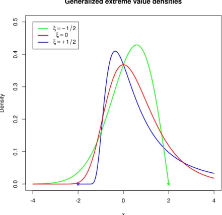
Denote this distribution as GEV(µ, σ, ξ). The shape parameterξ controls the tail of the distribution. When ξ > 0, the GEV distribution has a heavy, unbounded upper tail. When ξ = 0, this is commonly referred to as the Gumbel distribution and has a lighter tail. Figure 1.1 shows the GEV density for various shape parameter values.

Weissman (1978) generalized this result further, showing that the limiting joint dis-tribution of the r largest order statistics of a random sample of size B as B → ∞

(denoted here as the GEVr distribution) has probability density function

fr(y1, y2, ..., yr|µ, σ, ξ) =σ−rexp n −(1 +ξzr) −1 ξ − 1 ξ + 1 r X j=1 log(1 +ξzj) o (1.3)

for location parameter µ, scale parameter σ > 0 and shape parameter ξ, where y1 >

· · · > yr, zj = (yj −µ)/σ, and 1 +ξzj > 0 for j = 1, . . . , r. The joint distribution for ξ = 0 can be found by taking the limit ξ → 0 in conjunction with the Dominated Convergence Theorem and the shape parameter controls the tails of this distribution as discussed in the univariate GEV case. Whenr= 1, this distribution is exactly the GEV

(27)

Figure 1.1: The density function of the Generalized Extreme Value distribution for shape parameter values of −0.5, 0, and 0.5 with location and scale parameters fixed at zero and one, respectively.

distribution. The parameters θ = (µ, σ, ξ)> remain the same for j = 1, . . . , r, r B, but the convergence rate to the limit distribution reduces sharply as r increases. The conditional distribution of therth component given the topr−1 variables in (1.3) is the GEV distribution right truncated by yr−1, which facilitates simulation from the GEVr distribution; see Appendix A.1.

(28)

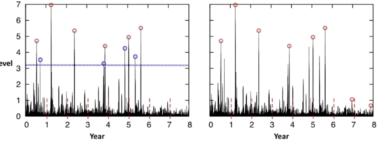
Figure 1.2: A comparison of extremes selected via the peaks over threshold (left) versus block maxima approach for example time series data.

1.1.2

Peaks Over Threshold (POT) Approach

Another approach to modeling extremes is the peaks over threshold method (POT). In-stead of breaking up the underlying data into blocks and extracting the top observations from each block, POT sets some high threshold and uses only the observations above the threshold. Thus, POT is only concerned with the relevant observations, regardless of temporal ordering. Figure 1.2 displays the differences between the POT and block maxima approaches.

Extreme value theory (McNeil and Saladin, 1997) says that given a suitably high threshold, data above the threshold will follow the Generalized Pareto (GPD) distri-bution. Under general regularity conditions, the only possible non-degenerate limiting distribution of properly rescaled exceedances of a thresholduis the GPD asu→ ∞(e.g.,

(29)

Pickands, 1975). The GPD has cumulative distribution function F(y|θ) =          1−h1 + _σξy u i−1/ξ ξ6= 0, y >0, 1 + _σξy u >0, 1−exph−_σy u i ξ= 0, y >0, (1.4)

where θ = (σu, ξ), ξ is a shape parameter, and σu > 0 is a threshold-dependent scale parameter. The GPD also has the property that for some threshold v > u, the excesses follow a GPD with the same shape parameter, but a modified scale σv =σu+ξ(v−u). Let X1, . . . , Xn be a random sample of size n. If u is sufficiently high, the exceedances

Yi =Xi−u for allisuch that Xi > uare approximately a random sample from a GPD. The GPD has the probability density function given by

f(y|σu, ξ) =          1 σu h 1 + _σξy u i−(1_ξ+1) , ξ 6= 0, 1 σuexp h − y σu i , ξ = 0. (1.5)

defined on y≥0 whenξ ≥0 and 0≤y ≤ −σu/ξ when ξ <0.

Both the block or threshold approach are justified in theory, but choice in application depends on the context or availability of data. For instance, it may be the case that only the block maxima or top order statistics from each period are available. The block maxima / r largest approach provides a natural framework in which to retain temporal structure, while the POT requires additional care. This may be important if interest is in modeling non-stationary extremes. Ferreira, de Haan, et al. (2015) provide an

(30)

overview of practical considerations when choosing between the two methods.

1.1.3

Non-stationary Regional Frequency Analysis (RFA)

Regional frequency analysis (RFA) is commonly used when historical records are short, but observations are available at multiple sites within a homogeneous region. A common difficulty with extremes is that, by definition, data is uncommon and thus short record length may make the estimation of parameters questionable. Regional frequency analysis resolves this problem by ‘trading space for time’; data from several sites are used in estimating event frequencies at any one site (Hosking and Wallis, 2005). Essentially, certain parameters are assumed to be shared across sites, which increases the efficiency in estimation of those parameters.

In RFA, only the marginal distribution at each location needs to be specified. To set ideas, assume a region consists of m sites over n periods. Thus, observation t at site s can be denoted as Yst. A common assumption is that data within each site are independent between periods; however, within each periodt, it is typically the case that there is correlation between sites. For example, sites within close geographic distance cannot have events assumed to be independent. Fully specified multivariate models generally require this dependence structure to be explicitly defined and it is clear that the dependence cannot be ignored. As noted by authors Stedinger (1983) and Hosking and Wallis (1988), intersite dependence can have a dramatic effect on the variance of these estimators.

(31)

There are a number of techniques available to adjust the estimator variances ac-cordingly without directly specifying the dependence structure. Some examples are combined score equations (Wang, 2015), pairwise likelihood (Wang et al., 2014; Shang, Yan, Zhang, et al., 2015), semi-parametric bootstrap (Heffernan and Tawn, 2004), and composite likelihood (Chandler and Bate, 2007).

1.2

Motivation

This thesis focuses on developing sound statistical methodology and theory to address practical concerns in extreme value applications. A common theme across the various methods developed here is automation, efficiency, and utility. There is a wide literature available of theoretical results and although recently the statistical modeling of extremes in application has gained in popularity, there are still methodological improvements that can be made. One of the major complications when modeling extremes in practice is deciding “what is extreme?”. The block maxima approach simplifies this idea somewhat, but for the POT approach, the threshold must be chosen. Similarly, if one wants to use the r largest order statistics from each block (to improve efficiency of the estimates), how isr chosen? Again, most of the current approaches do not address all three aspects mentioned earlier - automation, efficiency, and utility. For example, visual diagnostics cannot be easily automated, while certain resampling approaches are not scalable (effi-ciency), and many of the existing theoretical results may require some prior knowledge

(32)

about the domain of attraction of the limiting distribution and/or require computational methods in finite samples.

As data continues to grow, there is a need for automation and efficiency / scalability. Climate summaries are currently available for tens of thousands of surface sites around the world via the Global Historical Climatology Network (GHCN) (Menne, Durre, Vose, Gleason, and Houston, 2012), ranging in length from 175 years to just hours. Other sources of large scale climate information are the National Oceanic and Atmospheric Administration (NOAA), United States Geological Survey (USGS), National Centers for Environmental Information (NCEI), Environment and Climate Change Canada, etc. One particular motivating example is creating a return level map of extreme pre-cipitation for sites across the western United States. Climate researchers may want to know how return levels of extreme precipitation vary across a geographical region and if these levels are affected by some external force such as the El Ni˜no–Southern Oscillation (ENSO). In California alone, there are over 2,500 stations with some daily precipitation records available. Either using a jointly estimated model such as regional frequency analysis or analyzing data site-wise, appropriate methods are needed to accommodate modeling a large number of sites.

1.2.1

Choice of

r

in the

r

Largest Order Statistics Model

While the theoretical framework of extreme value theory is sound, there are many prac-tical problems that arise in applications. One such issue is the choice of r in the GEVr

(33)

distribution. Since r is not explicitly a parameter in the distribution (1.3), the usual model selection techniques (i.e. likelihood-ratio testing, AIC, BIC) are not available. A bias-variance trade-off exists when selecting r. As r increases, the variance decreases because more data is used, but ifris chosen too high such that the approximation of the data to the GEVr distribution no longer holds, bias may occur. It has been shown that the POT method is more efficient than block maxima in small samples (Caires, 2009) and thus it is often recommended to use that method over block maxima.

It appears that in application, the GEVr distribution is often not considered because of the issues surrounding the selection of r and that simply using the block maxima or POT approach are more straightforward. To the author’s knowledge, no comparison between efficiency of the GEVr distribution and POT method has been carried out in finite samples. In practice (An and Pandey, 2007; Smith, 1986) the recommendation for the choice of r is sometimes based on the amount of reduction in standard errors of the estimates.

Smith (1986) and Tawn (1988) used probability plots for the marginal distributions of the rth order statistic to assess goodness of fit. Note that this can only diagnose poor model fit at the marginal level – it does not consider the full joint distribution. Tawn (1988) suggested an alternative test of fit using a spacings result in Weissman (1978), however this requires prior knowledge about the domain of attraction of the limiting distribution. These issues become even more apparent when it is desired to fit the GEVr distribution to more than just one sample. This is carried out for 30 stations

(34)

in the Province of Ontario on extreme wind speeds (An and Pandey, 2007) but the value of r= 5 is fixed across all sites.

1.2.2

Selection of Threshold in the POT Approach

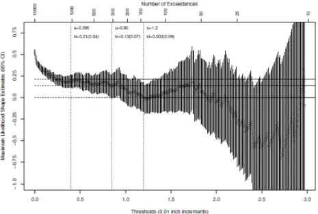
A similar, but distinct problem is threshold selection when modeling with the Gener-alized Pareto distribution. In practice, the threshold must be chosen, yet it cannot be chosen using traditional model selection tests since it is not a parameter in the distribu-tion. This has been studied thoroughly in the literature. Various graphical procedures exist. The mean residual life (MRL) plot, introduced by Davison and Smith (1990) uses the expectation of GPD excesses; for v > u, E[X−v|X > v] is linear in v when the GPD fits the data above u. The idea is to choose the smallest value of u such that the plot is linear above this point. The Hill estimator (Hill, 1975) for the tail index ξ is based on a sum of the log spacings of the top k+ 1 order statistics. Drees, De Haan, and Resnick (2000) discuss the Hill plot, which plots the Hill estimator against the top

k order statistics. The value of k is chosen as the largest (i.e. lowest threshold) such that the Hill estimator has become stable. A similar figure, referred to as the threshold stability plot, compares the estimates of the GPD parameters at various thresholds and the idea is to choose a threshold such that the parameters at this threshold and higher are stable.

It is clear that visual diagnostics cannot be scaled effectively. Even in the one sample case can be quite difficult to interpret, with the Hill plot being referred to as the ‘Hill

(35)

Figure 1.3: Mean Residual Life plot of Fort Collins daily precipitation data found in R packageextRemes.

Horror Plot’. Figures 1.3, 1.4, and 1.5 are examples of the mentioned plots applied to the Fort Collins daily precipitation data in R package extRemes (Gilleland and Katz, 2011a).

Some practitioners suggest various ‘rules of thumb’, which involve selecting the threshold based on some predetermined fraction of the data or it can involve com-plicated resampling techniques. There is also the idea of using a mixture distribution, which involves specifying a ‘bulk’ distribution for the data below the threshold and using the GPD to model data above the threshold. In this way, the threshold can be explicitly modeled as a parameter. There are some drawbacks to this approach however – the ‘bulk’ distribution must be specified, and care is needed to ensure that the two densities

(36)

Figure 1.4: Threshold stability plot for the shape parameter of the Fort Collins daily precipitation data found in R package extRemes.

Figure 1.5: Hill plot of the Fort Collins daily precipitation data found in R package

(37)

are continuous at the threshold pount u0.

Goodness-of-fit testing can be used for threshold selection. A set of candidate thresh-olds u1 < . . . < ul can be tested sequentially for goodness-of-fit to the GPD. The goal is to select a smaller threshold in order to reduce variance of the estimates, but not too low as to introduce bias. Various authors have developed methodology to perform such testing, but they do not consider the multiple testing issue, or it can be computa-tional intensive to perform. For a more thorough and detailed review of the approaches discussed in this section, see Scarrott and MacDonald (2012) and section 3.1.

1.2.3

Estimation in Non-stationary RFA

Unless otherwise noted, going forward the assumption is that the marginal distribution used in fitting a regional frequency model is the GEV or block maxima method. It is well known that due to the non-regular shape of the likelihood function, the MLE may not exist when the shape parameter of the GEV distribution, ξ < −0.5 (Smith, 1985). This can cause estimation and/or optimization issues, especially in situations where the record length is short. Even so, maximum likelihood is widely popular and relatively straightforward to implement. As an alternative, in the stationary RFA case, one can use L-moments (Hosking, 1990) to estimate the parameters in RFA. L-moments has the advantage over MLE in that it only requires the existence of the mean, and has been shown to be more efficient in small samples (Hosking, Wallis, and Wood, 1985). However, for non-stationary RFA, it is not straightforward to incorporate covariates

(38)

using L-moments, and generally MLE is used – see (Katz, Parlange, and Naveau, 2002; L´opez and Franc´es, 2013; Hanel, Buishand, and Ferro, 2009; Leclerc and Ouarda, 2007; Nadarajah, 2005) as examples.

One approach to estimate time trends is by applying the stationary L-moment ap-proach over sliding time windows (Kharin and Zwiers, 2005; Kharin, Zwiers, Zhang, and Wehner, 2013); that is, estimate the stationary parameters in (mutually exclusive) periods and study the change in parameters. This is not a precise method, as it is hard to quantify whether change is significant or due to random variation. In the one sample case, there has been some progress to combine non-stationarity and L-moment estima-tion. Ribereau, Guillou, and Naveau (2008) provide a method to incorporate covariates in the location parameter, by estimating the covariates first via least squares, and then transforming the data to be stationary in order to estimate the remaining parameters via L-moments. Coles and Dixon (1999) briefly discuss an iterative procedure to estimate covariates through maximum likelihood and stationary parameters through L-moments. However, these approaches only consider non-stationary in the location parameter and it may be of interest to perform linear modeling of the scale and shape parameters.

1.3

Outline of Thesis

The rest of this thesis is as follows. Chapter 2 builds on the discussion in Section 1.2.1, developing two goodness-of-fit tests for selection of r in the r largest order statistics

(39)

model. The first is a score test, which requires approximating the null distribution via a parametric or multiplier bootstrap approach. Second, named the entropy difference test, uses the expected difference between log-likelihood of the distributions of therand

r−1 top order statistics to produce an asymptotic test based on normality. The tests are studied for their power and size, and newly developed error control methods for order, sequential testing is applied. The utility of the tests are shown via applications to extreme sea level and precipitation datasets.

Chapter 3 tackles the problem of threshold selection in the peaks over threshold model, discussed in Section 1.2.2. A goodness-of-fit testing approach is used, with an emphasis on automation and efficiency. Existing tests are studied and it is found that the Anderson–Darling has the most power in various scenarios testing a single, fixed thresh-old. The same error control method discussed in Section 2.6 can be adapted here to control for multiplicity in testing ordered, sequential thresholds for goodness-of-fit. Al-though the asymptotic null distribution of the Anderson–Darling testing statistic for the GPD has been derived (Choulakian and Stephens, 2001), it requires solving an integral equation. We develop a method to obtain approximate p-values in a computationally efficient manner. The test, combined with error control for the false discovery rate, is shown via a large scale simulation study to outperform familywise and no error controls. The methodology is applied to obtain a return level map of extreme precipitation of at hundreds of sites in the western United States.

(40)

When analyzing climate extremes at many sites, it may be desired to combine infor-mation across sites to increase efficiency of the estimates, for example, using a regional frequency model. In addition, one may want to incorporate non-stationary. Currently, the only estimation methods available in this framework may have drawbacks in certain cases, as discussed in Section 1.2.3. In Chapter 4, we introduce two alternative meth-ods of estimation in non-stationary RFA, that have advantageous theoretical properties when compared to current estimation methods such as MLE. It is shown via simula-tion of spatial extremes with extremal and non-extremal dependence that the two new estimation methods empirically outperform MLE. A non-stationary regional frequency flood-index model is fit to annual maximum daily winter precipitation events at 27 lo-cations in California, with an interest in modeling the effect of the El Ni˜no–Southern Oscillation Index on these events.

Chapter 5 provides a brief tutorial to the companion software package eva, which implements the majority of the methodology developed here. It provides new imple-mentations of certain techniques, such as maximum product spacing estimation, and data generation and density estimation for the GEVr distribution. Additionally, it im-proves on existing implementations of extreme value analysis, particularly numerical handling of the near-zero shape parameter, profile likelihood, and user-friendly model fitting for univariate extremes. Lastly, a discussion of this body of work, and possible future direction follows in Chapter 6.

(41)

Chapter 2

Automated Selection of

r

in the

r

Largest Order Statistics Model

2.1

Introduction

The largest order statistics approach is an extension of the block maxima approach that is often used in extreme value modeling. The focus of this chapter is (Smith, 1986, p.28– 29): “Suppose we are given, not just the maximum value for each year, but the largest ten (say) values. How might we use this data to obtain better estimates than could be made just with annual maxima?” Ther largest order statistics approach may use more information than just the block maxima in extreme value analysis, and is widely used in practice when such data are available for each block. The approach is based on the lim-iting distribution of the r largest order statistics which extends the generalized extreme value (GEV) distribution (e.g., Weissman, 1978). This distribution, given in (1.3) and denoted as GEVr, has the same parameters as the GEV distribution, which makes it useful to estimate the GEV parameters when the r largest values are available for each

(42)

block. The approach was investigated by Smith (1986) for the limiting joint Gumbel distribution and extended to the more general limiting joint GEVrdistribution by Tawn (1988). Because of the potential gain in efficiency relative to the block maxima only, the method has found many applications such as corrosion engineering (e.g., Scarf and Laycock, 1996), hydrology (e.g., Dupuis, 1997), coastal engineering (e.g., Guedes Soares and Scotto, 2004), and wind engineering (e.g., An and Pandey, 2007).

In practice, the choice of r is a critical issue in extreme value analysis with the r

largest order statistics approach. In general r needs to be small relative to the block size B (not the number of blocks n) because as r increases, the rate of convergence to the limiting joint distribution decreases sharply (Smith, 1986). There is a trade-off between the validity of the limiting result and the amount of information required for good estimation. If r is too large, bias can occur; if too small, the variance of the estimator can be high. Finding the optimalr should lead to more efficient estimates of the GEV parameters without introducing bias. Our focus here is the selection of r for situations where a number of largest values are available each of n blocks. In contrast, the methods for threshold or fraction selection reviewed in Scarrott and MacDonald (2012) deal with a single block (n = 1) of a large size B.

The selection of r has not been as actively researched as the threshold selection problem in the one sample case. Smith (1986) and Tawn (1988) used probability (also known as PP) plots for the marginal distribution of the rth order statistic to assess its goodness of fit. The probability plot provides a visual diagnosis, but different viewers

(43)

may reach different conclusions in the absence of a p-value. Further, the probability plot is only checking the marginal distribution for a specific r as opposed to the joint distribution. Tawn (1988) suggested an alternative test of fit using a spacings results in Weissman (1978). Let Di be the spacing between the ith and (i+ 1)th largest value in a sample of size B from a distribution in the domain of attraction of the Gumbel distribution. Then {iDi : i = 1, . . . , r − 1} is approximately a set of independent and identically distributed exponential random variables as B → ∞. The connections among the three limiting forms of the GEV distribution (e.g., Embrechts, Kl¨uppelberg, and Mikosch, 1997, p.123) can be used to transform from the Fr´echet and the Weibull distribution to the Gumbel distribution. Testing the exponentiality of the spacings on the Gumbel scale provides an approximate diagnosis of the joint distribution of the

r largest order statistics when B is large. A limitation of this method, however, is that prior knowledge of the domain of attraction of the distribution is needed. Lastly, Dupuis (1997) proposed a robust estimation method, where the weights can be used to detect inconsistencies with the GEVr distribution and assess the fit of the data to the joint Gumbel model. The method can be extended to general GEVr distributions but the construction of the estimating equations is computing intensive with Monte Carlo integrations.

In this chapter, two specification tests are proposed to select r through a sequence of hypothesis testing. The first is the score test (e.g., Rao, 2005), but because of the nonstandard setting of the GEVr distribution, the usual χ2 asymptotic distribution

(44)

is invalid. A parametric bootstrap can be used to assess the significance of the ob-served statistic, but is computationally demanding. A fast, large sample alternative to parametric bootstrap based on the multiplier approach (Kojadinovic and Yan, 2012) is developed. The second test uses the difference in estimated entropy between the GEVr and GEVr−1 models, applied to the r largest order statistics and the r−1 largest order

statistics, respectively. The asymptotic distribution is derived with the central limit theorem. Both tests are intuitive to understand, easy to implement, and have substan-tial power as shown in the simulation studies. Each of the two tests is carried out to test the adequacy of the GEVr model for a sequence of r values. The very recently developed stopping rules for ordered hypotheses in G’Sell, Wager, Chouldechova, and Tibshirani (2016) are adapted to control the false discovery rate (FDR), the expected proportion of incorrectly rejected null hypotheses among all rejections, or familywise error rate (FWER), the probability of at least one type I error in the whole family of tests. All the methods are available in the R package eva (Bader and Yan, 2016) and some demonstration is seen in Chapter 5.

The rest of the chapter is organized as follows. The problem is set up in Section 2.2 with the GEVr distribution, observed data, and the hypothesis to be tested. The score test is proposed in Section 2.3 with two implementations: parametric bootstrap and multiplier bootstrap. The entropy difference (ED) test is proposed and the asymptotic distribution of the testing statistic is derived in Section 2.4. A large scale simulation study on the empirical size and power of the tests are reported in Section 2.5. In

(45)

Section 2.6, the multiple, sequential testing problem is addressed by adapting recent developments on this application. The tests are applied to sea level and precipitation datasets in Section 2.7. A discussion concludes in Section 2.8. The Appendices A.1 and A.2 contain the details of random number generation from the GEVr distribution and a sketch of the proof of the asymptotic distribution of the ED test statistic, respectively.

2.2

Model and Data Setup

The limit joint distribution (Weissman, 1978) of therlargest order statistics of a random sample of size B as B → ∞ is the GEVr distribution with probability density function given in (1.3).

The rlargest order statistics approach is an extension of the block maxima approach in extreme value analysis when a number of largest order statistics are available for each one of a collection of independent blocks (Smith, 1986; Tawn, 1988). Specifically, let (yi1, . . . , yir) be the observed r largest order statistics from block i for i = 1, . . . , n. Assuming independence across blocks, the GEVr distribution is used in place of the GEV distribution (1.2) in the block maxima approach to make likelihood-based inference about θ. Let l_i(r)(θ) =l(r)₍_y i1, . . . , yir|θ), where l(r)(y1, . . . , yr|θ) = −rlogσ−(1 +ξzr) −1 ξ − 1 ξ + 1 r X j=1 log(1 +ξzj) (2.1)

(46)

parameter µ, scale parameter σ > 0 and shape parameter ξ, where y1 > · · · > yr,

zj = (yj −µ)/σ, and 1 +ξzj > 0 for j = 1, . . . , r. The maximum likelihood estimator (MLE) of θ using the r largest order statistics is ˆθn(r)= arg maxPn_i₌₁l(_ir)(θ).

Model checking is a necessary part of statistical analysis. The rationale of choosing a larger value of r is to use as much information as possible, but not set r too high so that the GEVr approximation becomes poor due to the decrease in convergence rate. Therefore, it is critical to test the goodness-of-fit of the GEVr distribution with a sequence of null hypotheses

H₀(r): the GEVr distribution fits the sample of the r largest order statistics well

forr= 1, . . . , R, whereR is the maximum, predetermined number of top order statistics to test. Two test procedures for H₀(r) are developed for a fixed r first to help choose

r ≥ 1 such that the GEVr model still adequately describes the data. The sequential testing process and the multiple testing issue are investigated in Section 2.6.

2.3

Score Test

A score statistic for testing goodness-of-fit hypothesis H₀(r) is constructed in the usual way with the score function and the Fisher information matrix (e.g., Rao, 2005). For ease of notation, the superscript (r) is dropped. Define the score function

S(θ) = n X i=1 Si(θ) = n X i=1 ∂li(θ)/∂θ

(47)

and Fisher information matrix I(θ), which have been derived in Tawn (1988). The behaviour of the maximum likelihood estimator is the same as that derived for the block maxima approach (Smith, 1985; Tawn, 1988), which requiresξ >−0.5. The score statistic is Vn= 1 nS > (ˆθn)I−1(ˆθn)S(ˆθn).

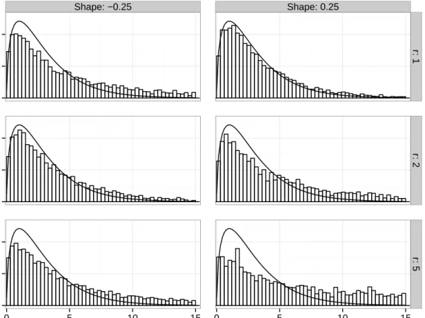
Under standard regularity conditions, Vn would asymptotically follow aχ2 distribu-tion with 3 degrees of freedom. The GEVr distribution, however, violates the regularity conditions for the score test (e.g., Casella and Berger, 2002, pp. 516-517), as its support depends on the parameter values unless ξ = 0. For illustration, Figure 2.1 presents a visual comparison of the empirical distribution ofVnwithn= 5000 from 5000 replicates, overlaid with the χ2(3) distribution, for ξ ∈ {−0.25,0.25} and r ∈ {1,2,5}. The sam-pling distribution ofVn appears to be much heavier tailed thanχ2(3), and the mismatch increases as r increases as a result of the reduced convergence rate.

Although the regularity conditions do not hold, the score statistic still provides a measure of goodness-of-fit since it is a quadratic form of the score, which has expectation zero under the null hypothesis. Extremely large values of Vn relative to its sampling distribution would suggest lack of fit, and, hence, possible misspecification of H₀(r). So the key to applying the score test is to get an approximation of the sampling distribution of Vn. Two approaches for the approximation are proposed.

(48)

Shape: −0.25 Shape: 0.25 0.0 0.1 0.2 0.0 0.1 0.2 0.0 0.1 0.2 r: 1 r: 2 r: 5 0 5 10 15 0 5 10 15 Score Statistic Density

Figure 2.1: Comparisons of the empirical vs. χ2_{(3) distribution (solid curve) based on}

5000 replicates of the score test statistic under the null GEVr distribution. The number of blocks used is n= 5000 with parameters µ= 0, σ= 1, and ξ ∈(−0.25,0.25).

2.3.1

Parametric Bootstrap

The first solution is parametric bootstrap. For hypothesisH₀(r), the test procedure goes as follows:

1. Compute ˆθn under H0 with the observed data.

2. Compute the testing statistic Vn.

(49)

(a) Generate a bootstrap sample of size n for the r largest statistics from GEVr with parameter vector ˆθn.

(b) Compute the ˆθn(k) under H0 with the bootstrap sample.

(c) Compute the score test statistic Vn(k).

4. Return an approximate p-value of Vn as L−1 PL

k=11(V (k)

n > Vn).

Straightforward as it is, the parametric bootstrap approach involves sampling from the null distribution and computing the MLE for each bootstrap sample, which can be very computationally expensive. This is especially true as the sample size n and/or the number of order statistics r included in the model increases.

2.3.2

Multiplier Bootstrap

Multiplier bootstrap is a fast, large sample alternative to parametric bootstrap in goodness-of-fit testing (e.g., Kojadinovic and Yan, 2012). The idea is to approximate the asymp-totic distribution of n−1/2I−1/2(θ)S(θ) using its asymptotic representation

n−1/2I−1/2(θ)S(θ) = √1 n n X i=1 φi(θ),

where φi(θ) = I−1/2(θ)Si(θ). Its asymptotic distribution is the same as the asymptotic distribution of Wn(Z, θ) = 1 √ n n X i=1 (Zi−Z¯)φi(θ),

(50)

conditioning on the observed data, where Z = (Z1, ..., Zn) is a set of independent and identically distributed multipliers (independent of the data), with expectation 0 and variance 1, and ¯Z = 1

n Pn

i=1Zi. The multipliers must satisfy R∞

0 {Pr(|Z1|> x)}

1

2dx <∞.

An example of a possible multiplier distribution is N(0,1).

The multiplier bootstrap test procedure is summarized as follows:

1. Compute ˆθn under H0 with the observed data.

2. Compute the testing statistic Vn.

3. For every k∈ {1, ..., L} with a large number L, repeat: (a) Generate Z(k)= (Z₁(k), . . . , Zn(k)) from N(0,1).

(b) Compute a realization from the approximate distribution of Wn(Z, θ) with

Wn(Z(k),θˆn).

(c) Compute Vn(k)(ˆθn) =Wn>(Z (k)_,_θ_ˆ

n)Wn(Z(k),θˆn).

4. Return an approximate p-value of Vn as L−1PL_k₌₁1(Vn(k) > Vn).

This multiplier bootstrap procedure is much faster than parametric bootstrap pro-cedure because, for each sample, it only needs to generate Z and compute Wn(Z,θˆn). The MLE only needs to be obtained once from the observed data.

(51)

2.4

Entropy Difference Test

Another specification test for the GEVr model is derived based on the difference in en-tropy for the GEVr and GEVr−1 models. The entropy for a continuous random variable

with density f is (e.g., Singh, 2013)

E[−lnf(y)] =−

Z ∞

−∞

f(y) logf(y)dy.

It is essentially the expectation of negative log-likelihood. The expectation can be ap-proximated with the sample average of the contribution to the log-likelihood from the observed data, or simply the log-likelihood scaled by the sample size n. Assuming that the r −1 top order statistics fit the GEVr−1 distribution, the difference in the

log-likelihood between GEVr−1 and GEVr provides a measure of deviation from H (r) 0 . Its

asymptotic distribution can be derived. Large deviation from the expected difference under H₀(r) suggests a possible misspecification of H₀(r).

From the log-likelihood contribution in (2.1), the difference in log-likelihood for the

ith block, Dir(θ) =l (r) i −l (r−1) i , is Dir(θ) = −logσ−(1 +ξzir) −1 ξ _{+ (1 +}_ξz ir−1) −1 ξ − 1 ξ + 1 log(1 +ξzir). (2.2) Let ¯Dr = _n1 Pn i=1Dir and SD2r = Pn

(52)

sample variance, respectively. Consider a standardized version of ¯Dr as

T_n(r)(θ) = √n( ¯Dr−ηr)/SDr, (2.3)

whereηr=−logσ−1 + (1 +ξ)ψ(r), andψ(x) = d log Γ(x)/dxis the digamma function. The asymptotic distribution ofTn(r)is summarized by Theorem 1 whose proof is relegated to Appendix A.2. This is essentially looking at the difference between the Kullback– Leibler divergence and its sample estimate. It is also worth pointing out thatTn(r)is only a function of the r and r−1 top order statistics (i.e., only the conditional distribution

f(yr|yr−1) is required for its computation). Alternative estimators of ηr can be used in place of ¯Dr as long as the regularity conditions hold; see Hall and Morton (1993) for further details.

Theorem 1. Let Tn(r)(θ) be the quantity computed based on a random sample of size

n from the GEVr distribution with parameters θ and assume that H(r

−1)

0 is true. Then

Tn(r) converges in distribution to N(0,1) as n → ∞.

Note that in Theorem 1, Tn(r) is computed from a random sample of size n from a GEVr distribution. If the random sample were from a distribution in the domain of attraction of a GEVr distribution, the quality of the approximation of the GEVr distribution to the r largest order statistics depends on the size of each block B → ∞

with r B. The block size B is not to be confused with the sample size n. Assuming

(53)

the r largest order statistics for the GEVr distribution. Since ˆθn is consistent forθ with

ξ >−0.5,Tn(r)(ˆθn) has the same limiting distribution as T (r)

n (θ) underH₀(r).

To assess the convergence ofTn(r)(ˆθn) toN(0,1), 1000 GEVrreplicates were simulated under configurations of r ∈ {2,5,10}, ξ ∈ {−0.25,0,0.25}, and n ∈ {50,100}. Their quantiles are compared with those ofN(0,1) via quantile-quantile plots (not presented). It appears that a larger sample size is needed for the normal approximation to be good for largerr and negativeξ. This is expected because larger rmeans higher dimension of the data, and because the MLE only exists for ξ >−0.5 (Smith, 1985). For r less than 5 andξ ≥0, the normal approximation is quite good; it appears satisfactory for sample size as small as 50. For r up to 10, sample size 100 seems to be sufficient.

2.5

Simulation Results

2.5.1

Size

The empirical sizes of the tests are investigated first. For the score test, the parametric bootstrap version and the multiplier bootstrap version are equivalent asymptotically, but may behave differently for finite samples. It is of interest to know how large a sample size is needed for the two versions of the score test to hold their levels. Random samples of size n were generated from the GEVr distribution with r ∈ {1,2,3,4,5,10}, µ = 0,

σ = 1, and ξ∈ {−0.25,0,0.25}. All three parameters (µ, σ, ξ) were estimated.

(54)

MLE. For the multiplier bootstrap score and ED test, the MLE only needs to obtained once, for the dataset being tested. However, in addition, the parametric bootstrap score test must obtain a new sample and obtain the MLE for each bootstrap replicate. To assess the severity of this issue, 10,000 datasets were simulated forξ ∈ {−0.25,0,0.25},

r∈ {1,2,3,4,5,10},n∈ {25,50}, and the MLE was attempted for each dataset. Failure never occurred for ξ ≥ 0. With ξ =−0.25 and sample size 25, the highest failure rate of 0.69% occurred for r = 10. When the sample size is 50, failures only occurred when

r= 10, at a rate of 0.04%.

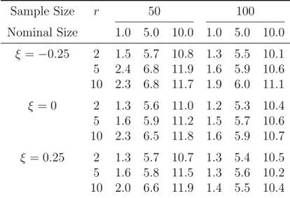
For the parametric bootstrap score test with sample size n∈ {25,50,100}, Table 2.1 summarizes the empirical size of the test at nominal levels 1%, 5%, and 10% obtained from 1000 replicates, each carried out with bootstrap sample size L = 1000. Included only are the cases that converged successfully. Otherwise, the results show that the agreement between the empirical levels and the nominal level is quite good for samples as small as 25, which may appear in practice when long record data is not available.

For the multiplier bootstrap score test, the results for n ∈ {25,50,100,200} are summarized in Table 2.2. When the sample size is less than 100, it appears that there is a large discrepancy between the empirical and nominal level. For ξ ∈ {0,0.25}, there is reasonable agreement between the empirical level and the nominal levels for sample size at least 100. For ξ =−0.25 and sample size at least 100, the agreement is good except for r = 1, in which case, the empirical level is noticeably larger than the nominal level. This may be due to different rates of convergence for various ξ values as ξ moves away

(55)

Table 2.1: Empirical size (in %) for the parametric bootstrap score test under the null distribution GEVr, with µ = 0 andσ = 1 based on 1000 samples, each with bootstrap sample size L= 1000. Sample Size r 25 50 100 Nominal Size 1.0 5.0 10.0 1.0 5.0 10.0 1.0 5.0 10.0 ξ=−0.25 1 0.4 2.8 6.0 1.1 4.8 9.3 0.6 4.1 8.0 2 0.1 2.6 6.0 0.8 3.4 6.5 0.6 3.6 8.1 3 0.3 2.5 5.0 0.8 4.3 7.7 1.1 4.8 8.1 4 0.3 1.8 5.4 0.6 3.1 6.9 1.1 5.1 8.8 5 0.4 2.4 6.7 0.4 3.3 8.3 0.6 3.1 6.5 10 2.7 5.3 8.7 0.5 3.9 8.4 0.7 4.2 7.6 ξ= 0 1 1.3 5.2 8.9 1.6 5.3 9.0 0.8 4.7 9.3 2 1.4 5.1 9.4 2.0 4.9 10.0 1.0 4.3 9.9 3 1.7 6.2 10.9 2.1 6.0 10.2 0.8 4.9 9.8 4 1.5 4.5 8.5 1.3 6.0 10.2 1.0 4.4 9.8 5 1.6 5.8 10.4 2.4 6.2 9.9 1.2 5.0 9.7 10 1.5 4.0 7.3 1.5 4.3 8.9 0.7 4.6 8.2 ξ= 0.25 1 1.7 4.5 9.7 2.6 7.1 11.5 1.1 4.6 9.1 2 1.8 5.1 8.7 1.8 4.4 8.5 0.5 2.9 7.5 3 1.5 4.4 9.4 1.5 3.7 8.1 1.0 4.2 9.4 4 1.2 3.3 8.1 1.1 4.6 9.7 1.1 4.3 9.6 5 1.7 4.4 9.4 1.1 4.2 8.6 0.6 4.8 9.6 10 1.1 4.6 8.3 1.5 6.1 10.7 1.0 3.9 8.5

from−0.5. It is also interesting to note that, everything else being held, the agreement becomes better asr increases. This may be explained by the more information provided by largerr for the same sample sizen, as can be seen directly in the Fisher information matrix (Tawn, 1988, pp. 247–249). For the most difficult case with ξ = −0.25 and

r= 1, the agreement gets better as sample size increases and becomes acceptable when sample size was 1000 (not reported).

(56)

Table 2.2: Empirical size (in %) for multiplier bootstrap score test under the null dis-tribution GEVr, with µ= 0 and σ = 1. 1000 samples, each with bootstrap sample size

L = 1000 were used. Although not shown, the empirical size for r = 1 and ξ =−0.25 becomes acceptable when sample size is 1000.

Sample Size r 25 50 100 200 Nominal Size 1.0 5.0 10.0 1.0 5.0 10.0 1.0 5.0 10.0 1.0 5.0 10.0 ξ=−0.25 1 7.0 13.4 18.9 6.3 13.8 19.6 5.4 11.4 16.3 5.4 10.5 15.2 2 2.0 6.9 13.4 1.3 6.4 12.4 1.6 6.9 13.6 1.4 6.7 12.8 3 2.1 5.8 11.7 1.1 5.9 11.1 1.1 5.0 10.8 1.5 5.9 11.8 4 3.3 7.2 12.3 1.1 4.9 10.8 1.0 5.2 11.9 1.1 5.6 10.6 5 3.6 9.0 14.0 2.3 6.8 11.2 1.1 6.2 10.6 1.1 4.5 9.3 10 2.0 7.0 10.3 2.6 7.4 12.8 2.1 6.4 10.1 1.4 6.4 11.6 ξ= 0 1 3.3 8.4 15.3 2.2 7.0 12.5 1.1 4.6 9.2 1.3 6.1 11.2 2 2.8 8.7 14.4 1.8 7.5 13.0 0.9 5.7 10.3 0.5 5.0 10.6 3 6.1 12.1 16.5 3.0 7.2 12.2 1.5 6.0 10.4 1.4 4.5 9.8 4 5.1 10.4 14.5 3.6 10.1 14.9 1.0 5.6 10.3 1.1 5.4 10.6 5 4.2 9.0 14.5 2.2 8.2 12.5 1.7 6.5 12.0 1.8 6.2 12.5 10 3.1 9.2 14.4 2.4 6.4 9.8 0.6 4.6 9.0 1.1 3.8 9.3 ξ= 0.25 1 1.8 6.7 13.7 1.3 4.7 10.4 0.8 4.4 11.5 0.9 4.9 11.4 2 5.7 12.7 17.1 4.7 9.9 14.9 3.5 7.4 11.6 3.2 7.9 11.7 3 7.1 12.2 16.5 5.3 9.4 14.8 4.2 8.4 12.5 1.8 6.1 10.7 4 5.4 9.8 16.8 3.7 9.0 13.4 2.6 6.0 11.4 1.2 4.9 11.2 5 4.4 10.1 15.8 3.5 8.2 13.6 2.4 7.4 11.4 1.6 5.9 10.0 10 3.3 8.9 15.3 2.4 6.6 12.3 1.6 5.8 10.9 1.7 6.6 12.4

To assess the convergence of Tn(r)(ˆθn) to N(0,1), 10,000 replicates of the GEVr dis-tribution were simulated with µ= 0 and σ = 1 for each configuration of r∈ {2,5,10},

ξ ∈ {−0.25,0,0.25}, and n ∈ {50,100}. A rejection for nominal level α, is denoted if |Tn(r)(ˆθn)| > |Zα₂|, where Zα₂ is the α/2 percentile of the N(0,1) distribution. Using this result, the empirical size of the ED test can be summarized, and the results are presented in Table 2.3.

For sample size 50, the empirical size is above the nominal level for all configurations ofrandξ. As the sample size increases from 50 to 100, the empirical size stays the same or decreases in every setting. For sample size 100, the agreement between nominal and

(57)

Table 2.3: Empirical size (in %) for the entropy difference (ED) test under the null distribution GEVr, with µ= 0 andσ = 1 based on 10,000 samples.

Sample Size r 50 100 Nominal Size 1.0 5.0 10.0 1.0 5.0 10.0 ξ=−0.25 2 1.5 5.7 10.8 1.3 5.5 10.1 5 2.4 6.8 11.9 1.6 5.9 10.6 10 2.3 6.8 11.7 1.9 6.0 11.1 ξ= 0 2 1.3 5.6 11.0 1.2 5.3 10.4 5 1.6 5.9 11.2 1.5 5.7 10.6 10 2.3 6.5 11.8 1.6 5.9 10.7 ξ= 0.25 2 1.3 5.7 10.7 1.3 5.4 10.5 5 1.6 5.8 11.5 1.3 5.6 10.2 10 2.0 6.6 11.9 1.4 5.5 10.4

observed size appears to be satisfactory for all configurations ofrand ξ. For sample size 50, the empirical size is slightly higher than the nominal size, but may be acceptable to some practitioners. For example, the empirical size for nominal size 10% is never above 12%, and for nominal size 5%, empirical size is never above 7%.

In summary, the multiplier bootstrap procedure of the score test can be used as a fast, reliable alternative to the parametric bootstrap procedure for sample size 100 or more when ξ ≥ 0. When only small samples are available (less than 50 observations), the parametric bootstrap procedure is most appropriate since the multiplier version does not hold its size and the ED test relies upon samples of size 50 or more for the central limit theorem to take effect.

(58)

2.5.2

Power

The powers of the score tests and the ED test are studied with two data generating schemes under the alternative hypothesis. In the first scheme, 4 largest order statistics were generated from the GEV4 distribution withµ= 0, σ= 1, andξ ∈ {−0.25,0,0.25},

and the 5th one was generated from a KumGEV distribution right truncated by the 4th largest order statistic. The KumGEV distribution is a generalization of the GEV distribution (Eljabri, 2013) with two additional parameters a and b which alter skew-ness and kurtosis. Defining Gr(y) to be the distribution function of the GEVr(µ, σ, ξ) distribution, the distribution function of the KumGEVr(µ, σ, ξ, a, b) is given byFr(y) = 1− {1−[Gr(y)]a}b for a > 0, b > 0. The score test and the ED test were applied to the top 5 order statistics with sample size n ∈ {100,200}. When a = b = 1, the null hypothesis of GEV5 is true. Larger difference from 1 of parametersaandb means larger

deviation from the null hypothesis of GEV5.

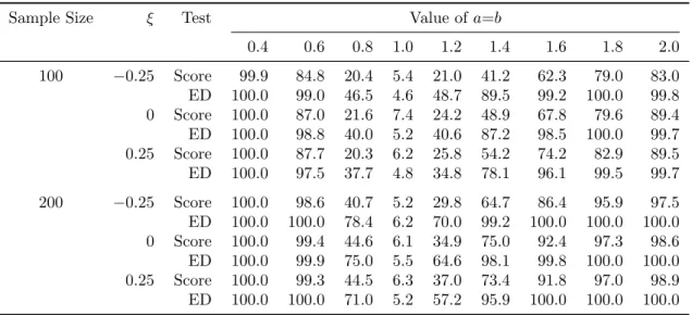
Table 2.4 summarizes the empirical rejection percentages obtained with nominal size 5%, for a sequence value of a =b from 0.4 to 2.0, with increment 0.2. Both tests hold their sizes when a =b = 1 and have substantial power in rejecting the null hypothesis for other values ofa =b. Between the two tests, the ED test demonstrated much higher power than the score test in the more difficult cases where the deviation from the null hypothesis is small; for example, the ED test’s power almost doubled the score test’s power for a = b ∈ {0.8,1.2}. As expected, the powers of both tests increase as a = b

(59)

Table 2.4: Empirical rejection rate (in %) of the multiplier score test and the ED test in the first data generating scheme in Section 2.5.2 from 1000 replicates.

Sample Size ξ Test Value ofa=b

0.4 0.6 0.8 1.0 1.2 1.4 1.6 1.8 2.0 100 −0.25 Score 99.9 84.8 20.4 5.4 21.0 41.2 62.3 79.0 83.0 ED 100.0 99.0 46.5 4.6 48.7 89.5 99.2 100.0 99.8 0 Score 100.0 87.0 21.6 7.4 24.2 48.9 67.8 79.6 89.4 ED 100.0 98.8 40.0 5.2 40.6 87.2 98.5 100.0 99.7 0.25 Score 100.0 87.7 20.3 6.2 25.8 54.2 74.2 82.9 89.5 ED 100.0 97.5 37.7 4.8 34.8 78.1 96.1 99.5 99.7 200 −0.25 Score 100.0 98.6 40.7 5.2 29.8 64.7 86.4 95.9 97.5 ED 100.0 100.0 78.4 6.2 70.0 99.2 100.0 100.0 100.0 0 Score 100.0 99.4 44.6 6.1 34.9 75.0 92.4 97.3 98.6 ED 100.0 99.9 75.0 5.5 64.6 98.1 99.8 100.0 100.0 0.25 Score 100.0 99.3 44.5 6.3 37.0 73.4 91.8 97.0 98.9 ED 100.0 100.0 71.0 5.2 57.2 95.9 100.0 100.0 100.0

In the second scheme, top 6 order statistics were generated from the GEV6

distribu-tion with µ = 0, σ = 1, and ξ ∈ {−0.25,0,0.25}, and then the 5th order statistic was replaced from a mixture of the 5th and 6th order statistics. The tests were applied to the sample of first 5 order statistics with sample sizes n ∈ {100,200}. The mixing rate

p of the 5th order statistic took values in {0.00,0.10,0.25,0.50,0.75,0.90,1.00}. When

p= 1 the null hypothesis of GEV5 is true. Smaller values of pindicate larger deviations

from the null. Again, both tests hold their sizes when p= 1 and have substantial power for other values of p, which increases as p decreases or as the sample sizes increases. The ED test again outperforms the score test with almost dou