This is an Open Access document downloaded from ORCA, Cardiff University's institutional
repository: http://orca.cf.ac.uk/126284/
This is the author’s version of a work that was submitted to / accepted for publication.
Citation for final published version:
Meng, Qinglong, Xiong, Chengyan, Mourshed, Monjur, Wu, Mengdi, Ren, Xiaoxiao, Wang,
Wenqiang, Li, Yang and Song, Hui 2020. Change-point multivariable quantile regression to explore
effect of weather variables on building energy consumption and estimate base temperature range.
Sustainable Cities and Society 53 , 101900. 10.1016/j.scs.2019.101900 file
Publishers page: http://dx.doi.org/10.1016/j.scs.2019.101900
<http://dx.doi.org/10.1016/j.scs.2019.101900>
Please note:
Changes made as a result of publishing processes such as copy-editing, formatting and page
numbers may not be reflected in this version. For the definitive version of this publication, please
refer to the published source. You are advised to consult the publisher’s version if you wish to cite
this paper.
This version is being made available in accordance with publisher policies. See
http://orca.cf.ac.uk/policies.html for usage policies. Copyright and moral rights for publications
made available in ORCA are retained by the copyright holders.
Title page:
Change-point multivariable quantile regression to explore
effect of weather variables on building energy consumption
and estimate base temperature range
Qinglong Meng1,2, Chengyan Xiong1, Monjur Mourshed2,Mengdi Wu1, Xiaoxiao Ren1,
Wenqiang Wang1, Yang Li1, Hui Song1
1School of Civil Engineering, Chang’an University, Xi’an, 710061, China
2School of Engineering, Cardiff University, Cardiff, CF24 3AA, United Kingdom
Corresponding author: Qinglong Meng (e-mail: [email protected]), Tel: (86)18229017219, URL: http://js.chd.edu.cn/jzgcxy/mql/list.htm
Change-point multivariable quantile regression to explore effect of
weather variables on building energy consumption and estimate base
temperature range
ABSTRACT: Mean regression analysis may not capture associations that occur primarily in the tails of the outcome distribution. In this study, we focused on building heating gas consumption related to multiple weather factors to find the extent to which they
impact gas consumption at higher quantile levels. We used change-point multivariable quantile regression models to investigate distributional effects and heterogeneity in the gas consumption-related responses to weather factors. Subsequently, we analyzed
quantile regression coefficients that corresponded to absolute differences in specific quantiles of gas consumption associated with a one-unit increase in weather factors. We found that the association of weather factors and gas consumption varied across 19
quantiles of gas consumption distribution. The heterogeneity of the case-study buildings was different: right tails of gas consumption for the community (CL) and educational (ED) buildings were more susceptible to weather factors than those of the
health care (HL) building. The base temperature of the CL building across quantiles of gas consumption indicated a flat trend, but the uncertainty ranges were relatively large compared with those for the CL and ED buildings. This study could reveal which
factors are most important and the extent to which they affect gas consumption at specific quantile levels.
Keywords: base temperature; building energy consumption; quantile regression; residual temperature; solar insolation.
2 1. Introduction
Urban energy consumption accounts for about 75% of global resource consumption. With urbanization accelerating in developing countries, the International Energy Agency predicts that by 2030, the share of urban energy demand will increase to
73% and CO2 emissions will increase to 76% [1]. Such rapid development of global industrialization, urbanization, and modernization has clearly increased the demand for energy. Reducing energy consumption and improving energy efficiency have
become urgent concerns for urban sustainable development. Buildings, in particular, are among the world's largest energy consumers [2]. Building energy accounts for 35-40% of society’s total energy consumption, which implies that there may be large
energy-saving potential in buildings. For example, energy-saving measures in buildings in the United Kingdom have reduced carbon dioxide emissions and saved up to 35% of energy. Therefore, energy-saving appliances and technologies should be
developed and used more widely. It is therefore desirable to reduce non-renewable energy requirements and the energy footprint of the built environment by developing new energy-saving technologies that are low cost and high reward. Diverse, innovative
technologies can also save additional energy. To meet requirements like thermal comfort, buildings are designed to deliver modulated amounts of energy to interior spaces. Both internal and external factors have effects on buildings. In addition to human
activities, weather conditions influence building energy use. More sustainable building protocols are needed to deal with climate change, which will depend on the innovation and development of energy-saving technologies. Weather parameters can be used
to predict indoor environmental conditions and establish sufficiently accurate prediction models. Building energy consumption performance can be quickly and accurately simulated using computer technology and prediction models [3]. Quantitative
representation of the relationship between energy consumption and weather conditions can provide necessary information for the development of new energy-saving technology. This relationship is also important for the short-term prediction of building energy,
and can help reduce building energy use before and after construction and /or retrofits.
A better understanding of the impacts of weather conditions on building energy use is needed to improve modeling and
prediction. Broadly speaking, forecasting can be classified into statistical, machine learning and physical methods [1]. In most prediction methods, the degree-day method, as an engineering mode, is based on one factor, i.e. temperature, providing an
inexpensive tool for building operators and managers. Climatic severity can be concisely characterized in terms of degree-days. According to Ref [2], the degree-day method is the simplest energy analysis method. The degree-day method can be used for
predicting building energy consumption [3], building design and regulations [4], as well as energy management [5]. Heating degree-day (HDD) is a versatile degree-day measure of cold weather duration and severity, allowing for weather-based analysis
of fuel consumption from sources such as natural gas or coal. In terms of degree-day, base or reference temperature is a key parameter. This is because base temperature influences the accuracy of HDD and corresponding energy consumption predictions.
Appropriate base temperatures are used to derive realistic representations of building energy consumption and efficiency, while
inappropriate choices can produce misleading results [6]. Furthermore, heating base temperature is temporal and dynamic change within a range rather than one point even if for a specific building [7].
The base temperature is generally determined by the energy signature method or the performance line method, the former method needs denser data sampling frequency (such as daily energy consumption readouts) than the latter method (often needs
monthly measurements). Currently, detail utility bills are easy to come by, and historic weather data are ubiquitous. Thus, the energy signature method is convenient to use. Much previous work has been done on the determination of base temperature using
the two approaches as well as on the practical issues with analyzing energy use data [8, 9, 10, 11, 12]. Other methods for estimation of base temperature were reported in Ref [13, 14]
Change-point model (CP) [15] has been further developed into estimating the change of patterns in a CP regression model which has had widespread use as baseline models for measuring energy savings. Due to simplicity, change-point (CP) model is
proved to be the most appropriate model in terms of accuracy vs. effort spent for verification of whole building energy consumption, and estimating building parameters [16]. One of model, best-fit change-point model, from American Society of
Heating, Refrigerating, and Air-conditioning Engineers (ASHRAE) Inverse Modeling Toolkit (IMT) [17] is used to derive regression models of building energy use.
Building energy consumption is weather-dependent [18]. As an engineering method, HDD is a versatile climatic indicator that encapsulates the severity and duration of cold weather. The existing methodologies only account for the effects of temperature
and ignore other potential climatic factors such a humidity, wind speed, and solar radiation. Because buildings are exposed to the environment, however, additional weather variables should be considered along with ambient temperature when determining base
temperature using a regression method. Although much research has been conducted on degree-days and determining base temperature, most studies [19, 20] have focused on one parameter (e.g. temperature) and only limited studies have incorporated
more than one into the approach. Sonderegger [21] derived a baseline model for utility bill analysis considering weather and non-weather- (i.e., occupancy) related variables. Guan [22] incorporated residual temperature (the temperature difference
between the current and the previous day’s temperature) and specific humidity to predict weather-dependent electricity consumption in the warm season. In Ref. [23] a new concept (infiltration degree-days (IDD)) was proposed, which added a
weighting factor calculated from relative infiltration. Huang [24] correlated residential building heating and cooling loads with different climatic parameters based on hourly simulated data. Stronger correlations were obtained using two parameter daily
4
effects of multiple climatic factors on the degree-days method were considered, such as temperature, humidity, and solar
radiation.
Building technologies are often examined by a mean regression approach. However, research questions can often go beyond
what can be answered in a standard regression framework. Previous studies have shown evidence of multi-variable dependency and heterogeneity in the relationship between the energy consumption distribution and different weather factors. Common
analytic approaches to examine energy consumption dependency on weather (especially ambient temperature) and further estimate base temperature include energy signature and performance line methods [3], which made improvements over classical
methods, such as quantile-quantile plots [13] and Bayesian estimation [14]. However, these approaches are all based on one parameter, such as temperature, as well as ordinary least squares (OLS) mean regression. Accordingly, they have not provided
sufficient understanding of how weather factors change the distribution of energy consumption. In particular, if larger energy consumption were seen among buildings at the adverse end of such distributions, such findings would have important energy
conservation implications and be helpful for energy use impact assessments and building performance analysis. Investigating variations in energy consumption effects based on the outcome of interest has received less attention but would address the issue
of fully understanding the reasons for changes in the distribution of actual energy use.
Quantile regression, introduced by Koenker and Bassett, provides “a systematic strategy for examining how covariates
influence the location, scale, and shape of the entire response distribution” [26], which is different from the classical least-squares regression only on the conditional mean. Quantile regression offers, on a systematic level, a more comprehensive distribution
picture of the relationship between the variables than ordinary regression does [27]. In terms of HDD-based building energy predictions, the advantages of quantile regression mainly are in following aspects. First, QR approach could provide with a wealth
of information across buildings energy use and weather, and can identify energy use anomalies in system behavior (for example, due to control failure or unrelated-weather occupant behavior) and poor-quality data. Second, quantile regression also has
flexibility in detecting more subtle relationships between energy use and ambient temperature, dealing with non-normally distributed errors, robustness against outliers, and the ability to detect heterogeneity (e.g., the distribution of gas consumption).
Finally, current studies on base temperature mostly focus on average using the conditional mean function. Unlike classical statistical regression methods, the outcomes of quantile regression are not only point estimates, but a full picture of base
temperature.
Obviously, the use of quantile regression (QR) allows for the examination of questions of differential relations or importance
while avoiding the problems associated with assuring a normal distribution or filtering skewness points. The main attraction of QR is that different measures of central tendency and statistical dispersion are available to make the analysis more comprehensive.
While until now research efforts on QR in building energy use is nascent, some limited implementation examples provide early
evidence of its potential. For instance, to determine the control limit on energy end use, QR with principal components analysis was applied [28], and Kaza adopted QR analysis to tease out the effects of various factors over the energy consumption spectrum
[29]. However, this approach has been frequently deployed in other fields, such as economics, social science, and environmental science [27, 30, 31]. The obstacle for application of the approach to energy conservation may be how to transfer QR results to
useful tools for building energy management. In [32], distributional degree-day temperatures were obtained using change point quantile regression where single outdoor environmental factor, i.e., ambient temperature, was considered.
In conclusion, from the literature it can be learned that, 1) the above studies all suggest that base temperature is highly dependent on building characteristics and operating conditions (by only using measured data from operating days). Although we
know that base temperature is characterized by multi-variable dependency and spatial and temporal distributions, few comprehensive studies have evaluated it. 2) Current studies on base temperature mostly focus on average using the conditional
mean function. To the best of the author’s knowledge, except [32], the analysis on the relationship between degree-day base temperatures and building consumption using quantile regression has not yet been investigated systematically.
Unlike classical statistical regression methods, the outcomes of quantile regression are not only point estimates, but a full picture of base temperature. Multivariable change-point quantile regression method energy analysis could examine some key
consumption drivers (in particular, e.g., solar simulation) and be further helpful to the development of predictive algorithms to estimate energy consumption and savings. Furthermore, in addition to knowing the relationship between mean energy
consumption and weather factors, we need more details, such as which part of the energy consumption is more susceptible to which weather factors, which cannot be achieved by OLS mean regression method.
The data for building information, weather (including weather derivatives such as residual temperature, the difference between the current and the previous day’s temperature), and energy use (gas consumption) and the methodology are first
described in detail. Using a change-point multivariable quantile regression (CP-MQR) approach, we subsequently discuss the association of daily average weather factors with 5th to 95th quantiles of the gas consumption distribution for three case-study
buildings. Finally, we compare results of QR from the three buildings to evaluate our conclusions.
2. Methodology
2.1 Data
2.1.1 Energy consumption
To evaluate the proposed method, we selected three non-residential buildings in Cardiff, South Glamorgan County, UK. The selected buildings represent diverse building sectors: community center (CL), educational (ED) building, and health care (HL)
6
building. The maximum distance between the weather station providing the meteorological data (Bute Park, Cardiff) and buildings
is less than 3.0 km. The detailed characteristics of the case-study buildings are listed in Table 1.
TABLEI
CASE-STUDY BUILDINGS CHARACTERISTICS
Building code CL ED HL
Photos
Building sectors1 Community, arts and leisure Education Health
Sub-sectors1 Clubs and community centres Primary school Nursing and care homes
Floor area (m2) 772 2437 317
Occupancy number (-) N/A2 387 33
Floor number (-) 1 2 2
Year built (-) Post 1976 Pre 1919 Post 1976
Occupancy schedule
09:30-21:30 (weekdays) 10:30-17:30 (Saturday) 11:00-15:30 (Sunday)
09:00-17:00 (weekdays 24h (weekdays and weekend)
Display Energy Certificate D C N/A
Note: 1 Buildings are categorized according to the Building Energy Efficiency Survey (BEES) [33], 2 N/A means that the variable is not available
Energy data for this research were gleaned from the City of Cardiff Council1, which monitors the gas and electricity
consumption of over 330 non-residential buildings and facilities they own and manage, as part of their sustainable development strategy. Energy consumption is measured every half-hour and sent to a central server. Some of these data are also publicly
available in Carbon Culture,2 a community platform for promoting the efficient use of resources. The raw data include energy
utility bills for both electricity and gas for periods with different starting and ending dates. As an example of building energy
consumption, we selected the gas consumption of three buildings covering 4 years from April 1, 2012, to March 31, 2016. The raw half-hourly gas consumption data were directly converted to daily equivalents for further analysis. Carpet plots were
prepared for various time frames, allowing us to identify patterns easily by visual inspection. Fig.1 illustrates carpet plots of gas consumption for the three buildings. Gas consumption had seasonal and diurnal patterns of dependency on the variation of ambient
temperature. Due to different functions and occupancy schedules, the diurnal patterns of three buildings had different characteristics. As an example, Fig.1b reveals that the peak heating demand fell within the time period of late October to early
April and from 7:00 to 17:00. In the daytime, the peak heating demand centered around 8:00, and lower heating demand was seen
1 The governing body for Cardiff, which is the capital of Wales. https://www.cardiff.gov.uk 2 https://platform.carbonculture.net/communities/car
before 7:00 and after 15:00. In most unoccupied periods (weekends and holidays), there was almost no energy use. Furthermore,
compared with the CL (Fig.1a) and ED (Fig.1b) buildings, the HL building (Fig.1c) had a relatively distinct heating system starting and ending cycle, which reflected a relatively stricter building operation management.
FIGURE 1. The carpet plot of gas consumption for three selected case buildings corresponding to three building types. a. Community Hall (Community, arts and leisure, CL). b. Primary school (Education, ED). c. Nursing and home care (Health, HL).
While the process is illustrated here using gas consumption, other energy end uses, such as heating, air-conditioning plug loads,
mechanical systems (fans and pumps), lighting, and even photovoltaic power generation, can be analyzed using our approach.
2.1.2 Weather
Three candidate weather stations were available for South Glamorgan: Bute Park, Rhoose, and St. Athan, located in the CF1, CF6, and CF64 Cardiff postal codes, respectively. Bute Park (latitude 51.4878 and longitude -3.18728, assigned World
Meteorological Organization [34] number 037170 and marked with a black solid circle in Fig.1) was chosen as the source station, as it is located within 1 km of the Cardiff city center. The average distance between the selected buildings and Bute Park weather
station is around 1.83 km (See in Fig.2). Bute Park is an automatic weather station that logs and reports weather parameters hourly. The remaining two stations, Rhoose and St. Athan (World Meteorological Organization numbers 037150 and 037160,
respectively, not shown in Fig.2), are located at nearby airports far from the city and have landscape characteristics different than those at the selected buildings, in terms of surroundings, built up areas, and exposure.
8 FIGURE 2. Maps of three case-study buildings and weather stations (Bute Park, Cardiff).
Hourly weather data from Cardiff were obtained from the Centre for Environmental Data Analysis [35], which archives data from the UK Met Office’s network of weather stations as part of the Met Office Integrated Data Archive System, Land and Marine
Stations dataset. The raw hourly data downloaded from the Centre often have duplicate and missing data. Therefore, pre-processing for duplicates and missing observations was conducted on the downloaded data to acquire complete and accurate data.
The carpet plots of post-processed hourly weather data, that is, air temperature, solar insolation, and residual temperature, are shown in Fig.3 for the study period. Residual temperature can be expressed as:
∆��,�=�� ‒ �‒ �� (1)
Where ∆��,� is the residual temperature in the th day resulting from the (� � ‒ �)th day.
As seen from Fig.3, the ambient temperature and solar insolation show seasonal and diurnal variation, while the variation of residual temperature looks more random. As an example of ambient temperature, the range of hourly ambient temperatures over
4 years was between -5°C and 30°C. The lowest ambient temperature occurred mainly around a time of day of 5:00 between November and March. Meanwhile, the highest temperature occurred at around 15:00. All of the weather parameters were tabulated
on an hourly basis, to maintain consistency with well-known terms of heating degree-days, although we converted the climatic parameters to daily equivalents when correlating building energy consumption and weather parameters.
FIGURE 3. The carpet plot of gas consumption for three selected case buildings corresponding to three building types. a. Community Hall (Community, arts and leisure, CL). b. Primary school (Education, ED). c. Nursing and home care (Health, HL).
2.2 Statistical approach
2.2.1 Change-point model for heating
The functional form of a best-fit three-parameter change-point model for heating is given as
�h=�1+�1
(
�b‒ �1)
+, (2)where �h is energy use (gas consumption in kilowatt-hours); �1is ambient dry bulb temperature (in degrees Celsius); �1 is baseline energy consumption or base load, the part of energy use that is independent of weather conditions; �1 is the physically meaningful slope of the total heat loss coefficient; and is the reference�b or base temperature (in degrees Celsius). The (+) notation indicates that the value of the parenthetical term is set to zero when it is negative. Using the three parameters, heating regression analysis can identify the breakpoint, that is, change-point (e.g., the blue point P shown in Fig.4a).
FIGURE 4. Schematics featuring the regression models of (a) 3PH change-point regression, (b) multi-variable 3PH change-point quantile regression (two independent variables).
In addition to ambient temperature, other climatic factors need to be considered when correlating building energy consumption dependency on weather for the improvement of estimation accuracy. Accordingly, multi-variable regression models are employed.
Although an ordinary multi-variable regression model can capture the effects of multiple independent variables, it cannot model energy use that varies at ambient temperature change points and balance points. The combination of change-point and
10
the effects of additional independent variables. Consequently, as in [17], we used the following three-parameter CP-MQR model
for heating:
�h=�1+�1
(
�b‒ �1)
+ +�2�2+�3�3+�4�4, (3)where �1 is ambient temperature and �� (�= 2, 3, 4) is one or more optional independent variables.
The OLS model can estimate how, on average, these independent variables affect the energy use. While the OLS model can address the question, for example, “is solar insolation important?” it cannot answer important questions such as “Does solar
insolation influence energy use differently at low consumption than it does for average or high consumption?” Fortunately, a more comprehensive picture of the effects of independent variables on the dependent variable can be obtained by using QR.
2.2.2 Quantile regression model: the preliminaries
Quantile regression, introduced by Koenker and Bassett [26], is different from OLS regression only with respect to the
conditional mean. Quantile regression offers, on a systematic level, a more comprehensive distribution picture of the relationship between the variables than ordinary regression does [27]. This approach can be applied to each quantile of the distribution function
separately, and therefore, it is more robust in handling outliers and applicable to asymmetrical distributions [36]. An interesting feature of this method is that no assumption is required about the probability distribution of the measurements as the function
parameters are estimated by a non-parametric technique that consists of minimizing asymmetrically weighted absolute residuals as the following linear equation:
min � �
∑
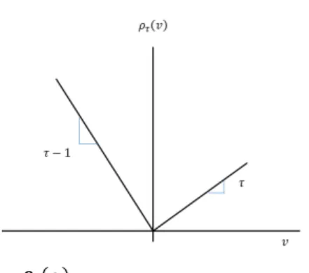
�= 1 ��(��‒ ����), (4)where is a scalar-dependent variable, � ��� is the �× 1 vector of explanatory variables, is the coefficient vector, is the � � conditional quantile of interest, and ��(�) =�(� ‒ �(�< 0)), 0 <�< 1, is the QR loss function [27] as shown schematically in Fig.5. Here, �(∙) denotes the indicator function.
FIGURE 5. Loss function for quantile regression ��(∙)
Quantile regression models the relation between a set of predictor variables and specific quantiles of the response variable. For
use as a function of the predictors. The effect of one predictor on median energy use can be compared with its effect on other
quantiles of energy use. In linear regression, the regression coefficient represents the increase in the dependent variable produced by a one-unit increase in the independent variable associated with that coefficient. In QR regression, the QR regression coefficient
estimates the change in a specified quantile of the dependent variable produced by a one-unit change in the independent variable. For example, this allows analysis of how some quantiles of energy use may be affected by some weather factors more than others.
This is reflected in the change in the size of the regression coefficient. Hence, the use of QR over the entire range of an outcome (building energy consumption) produces estimates that can be used to detect potential heterogeneity in weather–outcome
associations according to outcome levels. Another advantage of QR is that it does not require assumptions about the distribution of the outcome (or the model residuals) and can, therefore, be deployed to estimate associations between weather and building
energy consumption that are not normally distributed.
2.2.3 Change-point multivariable quantile regression: the extensions
The detailed theory of linear QR can be found in Refs. [26, 27]. From the above discussion of the energy signature model, we
know that linear QR lacks the ability to describe the relationship between energy use and ambient temperature and infer base temperature, while segmented linear QR may be preferable. Using the piecewise linear regression method, a more accurate range
of base temperatures for a specific building can be obtained, unlike a single estimated point obtained by the OLS method. Following previous studies on bent line QR [27, 37, 38, 39], we extensively developed the CP-MQR method.
Given a probability strictly between 0 and 1, we consider a three-parameter CP-MQR model derived from (2) (shown in � Figure 4b).
��=�1+�1
(
�b‒ ��)
+ +�⊺��+�� , (5)where is the -th response, is the scalar covariate whose slope changes at the change-point ,�� � �� �b �� is a -dimensional vector� of linear covariates with constant slopes, is the error term whose -th quantile is zero conditional on (�� � ��, ��), is the effect of �
, is an unknown variable to be estimated, and . The (+) notation indicates that the values of the parenthetic term is
�� �� �= 1,⋯,�
set to zero when it is negative. Let�= (�1,�1,�⊺)⊺. Given , the -th quantile of given and �� � �� �� ��, �(��,��;�)is .
�(��,��;�) =�1+�1
(
�b‒ ��)
+ +�⊺�� (6)As is known in (6), then, conditional on this known , the best estimate �� �� � �of is
�(�) = argmin� ∈ ℝ2 +�
�
∑
�= 1
��[��‒ �(��,��;�)]. (7)
12
��=�(��,��;�) =�1+�1��+�⊺�� . (8)
As (7) is equivalent to (6), (7) can be rewritten as
�= argmin� ∈ ℝ2 +�
�
∑
�= 1
��(��‒ ��,�⊺��), (9)
where ��,�b= (1,��,�⊺�)⊺. Now we can estimate �conditional on�b. As in [37], we adopted S(�|�b) (a function of ) as the following equation:�b
S
(
�│
�b)
= �∑
�= 1
��
(
��‒ ��,⊺�b�)
. (10)Finally, we can obtain all values of S(�|��) corresponding to all values of in the range of �� ��'s. The estimated change-point value , the value at which the minimum value of �b �b S(�|��) is realized, is calculated through the following equation:
��= argmin�
b
S(�|��). (11)
Both asymptotic and bootstrapping methods provide robust results for standard errors and confidence limits for regression
coefficient estimates [40]. We used the bootstrap technique for deriving confidence intervals (CIs) of the derivative of a QR model as more practical [41]. The triplets of variables (� �1, ��, and �1) with replacement from {��, ��, ��)|�= 1, ⋯, �|} were resampled, and these bootstrap samples were then used to re-estimate �1, ��, and �1. We calculated the 95% CIs for parameters �1, �b, and
using the bootstrap method [42]. Data were resampled and replaced 200 times.
�1
These quantile models are useful when the response variable is affected by more than one factor, when not all factors are measured, when factors vary in their effect on the response, or when multiple limiting factors interact [43]. Hence, similar to (3),
a three-parameter CP-MQR model could be derived from (5) (see Fig.2b for an example with two independent variables).
��=�1+�1
(
�b‒ �1�)
+ +�2�2�+�3�3�+�4�4�+�⊺��+��, (12)where �1� is the scalar covariate whose slope changes at the change-point ��,��� (�= 2, 3, 4) is one or more optional independent variables, and �= 1,⋯,�.
3 Results and discussion
3.1 Descriptive statistics
Cardiff has an essentially temperate oceanic climate with direct influences from the ocean, and the weather there is mild and often cloudy, wet, and windy. Winters tend to be fairly wet, but rainfall is rarely excessive, and the temperature usually stays
above freezing3. Fig.6 illustrates the relationships between gas consumption and weather factors, that is, daily mean dry-bulb
temperature, daily solar insolation, and residual temperature, for the case-study buildings. The number of measurements for all variables is 1,461. The gas consumption data contain some anomalies (such as the skewness points enclosed by red dashed circles
in Fig.6, panels a1, b1, and c1) which may have resulted from data collection errors (sensor faults), control faults (wide control dead bands or lack of weather-related controls), or operational factors. In addition, we observed that the negative effects of
temperature on gas consumption appeared to be stronger in the higher gas consumption measured for the ED building (Fig.6, panel b1).
FIGURE 6. Weather factors vs gas consumption for three case-study buildings
Spearman correlations between weather factors and gas consumption for the three case-study buildings during the study period
are presented in Table 2. Temperature was positively correlated with solar insolation (�= 0.53). We found no statistically significant correlation between the other weather factors. Consistent with the results shown in Table 2, gas consumption for all
case-study buildings was significantly negatively correlated ( �≈ 0.80) with temperature. In contrast, the associations with solar insolation were relatively weaker, and those with residual temperature revealed no statistically significant correlation.
TABLE II
SPEARMAN CORRELATIONS ( )� FOR THE WEATHER FACTORS AND GAS CONSUMPTION Gc Variable At Si Rt CL ED HL At 1 0.534 -0.175 -0.813 -0.788 -0.874 Si 1 0.006 -0.526 -0.490 -0.529 Rt 1 0.005 -0.036 0.072 Gc 1 1 1
At = Ambient temperature, Si = Solar insolation, Rt = Residual temperature, Gc = Gas consumption.
14
The CP-MQR models were estimated for the 5th to 95th quantiles in increments (τ) of 5 to test for heteroscedasticity across the entire distribution of the quantiles for the three case-study buildings. Also, OLS regressions with the same variables were calculated for comparing potential differences with the CP-MQR distribution from the lower to upper tails.
For the CL building (Fig.7), our results showed that the association between gas consumption and the three weather factors was not generally homogenous across quantiles. Fig.7 suggests increased gas consumption in response to decreases in temperature,
solar insolation, and residual temperature. We observed that the negative association between all three weather factors and gas consumption was stronger in the higher quantiles of the gas consumption. For instance, a one-unit increase in temperature was
associated with a 15.1 kWh decrease (95% CI: 14.1, 16.0) in the 10th quantile of gas consumption, and was significant in the 90th quantile (50.0 kWh/°C, 95% CI: 48.0, 52.3) (Fig.7b). Although the association between residual temperature and gas consumption
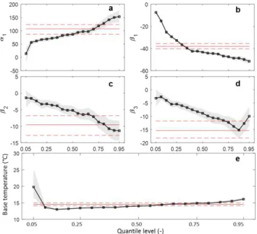
became stronger with increasing quantile up to the 85th quantile, above the 85th quantile, the association became weaker (the absolute value of �3 was lower, Fig.7d). Base building load �1 was positively correlated across all quantiles of gas consumption (Fig.7a). Additionally, it is worth noting that the pattern of changes in the estimated �1(�) ( denotes quantile) mirror those for � other coefficients (especially for �3 in Fig.7c). Except for the extreme 5th quantile, which is always influenced by outliers, base temperature slowly increased from the 10th to 95th quantiles of the outcome, over a range from 13.6°C to 16.1°C (Fig.7e). �b
FIGURE 7. Estimated coefficients from multivariable change-point quantile regression and OLS regression for CL building. The point-wise 95% confidence bounds are shown in grey areas. Each solid red line is coefficient from an OLS regression and the dashed red lines delineate the 95% point-wise confidence band based on bootstrap quantiles about this coefficient. Note: �� denotes base load. ���=�,�,� denotes slope coefficients, indicating the association between gas consumption and ambient temperature, solar insolation and residual temperature, respectively.
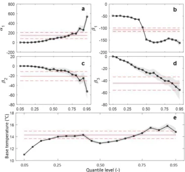
For the ED building (Fig.8), although weather factors were not significantly associated with the lower quantiles of gas
became stronger with increasing quantile. For instance, we saw little negative solar insolation–gas consumption association
(namely, almost null associations for the 5th to 40th quantiles; see coefficient �2 in Fig.8c). However, results suggested stronger negative effects of solar insolation at higher gas consumption quantiles (above the 60th quantile) that were relatively flat over the
distribution, in contrast with �3 estimates. The magnitude of �3 (Fig.8d) increased monotonously from the 5th quantile (0.0°C/kWh, 95% CI: 0, 0) to the 95th quantile (-55.8°C/kWh, 95% CI: -72.6, -39.2). Also, ambient temperature had relatively little relation to lower gas consumption quantiles (<40th quantile, with a magnitude of around 50°C/kWh); nevertheless, the
association rapidly became stronger above the 45th quantile and increased to an absolute value of around 150°C/kWh (Fig.8b). Note that the pattern of changes in �2(�) mirror those for �1(�) (Fig.8c and 8a). As a result, base temperatures (Fig.8e) showed random variations across all quantiles (12.3–15.8°C across the 10th to 90th quantiles).
FIGURE 8. Estimated coefficients from multivariable change-point quantile regression and OLS regression for ED building. The point-wise 95% confidence bounds are shown in grey areas. Each solid red line is coefficient from an OLS regression and the dashed red lines delineate the 95% point-wise confidence band based on bootstrap quantiles about this coefficient.
Different from the CL and ED buildings, for the HL building (Fig.9), we found no obvious distributional distortions on the
slope coefficients , which is consistent with our analysis that found no evidence against homogeneous associations over the gas � consumption distribution. For example, Fig.9c shows that the solar insolation–gas consumption association was fairly
homogenous (i.e., no clear monotonic patterns across quantiles of gas consumption, excluding both distribution tails). Moreover, except for the lowest quantile, �1 and �2 (Fig.9b and Fig.9c) had no clear relative variations across all quantiles, and the base temperature estimates (Fig.9e) also indicated a similar trend (14.0–13.4°C across the 10th to 90th quantiles). On the contrary, base
16 FIGURE 9. Estimated coefficients from multivariable change-point quantile regression and OLS regression for HL building. The point-wise 95% confidence bounds are shown in grey areas. Each solid red line is coefficient from an OLS regression and the dashed red lines delineate the 95% point-wise confidence band based on bootstrap quantiles about this coefficient.
Overall, consistent with the theory, we observed that all associations between weather factors and gas consumption were
negative for the three buildings. In addition, we noted that the QR coefficients tend to have greater variance when estimated at the tails of the distributions, which may be due to fewer observations at the tails (compared with the center) employed in the QR.
3.3 Discussions
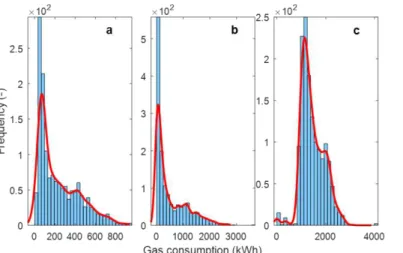
Our findings show heterogeneous associations across all quantiles of the gas consumption distribution for different building types and further suggest potentially different impacts of weather factors on gas consumption at different quantile levels. Therefore,
the heterogeneity extents for different buildings are different, indicating consistency with the gas consumption distribution shown in Fig.10. The results of QR for the CL and ED buildings revealed strong heterogeneity in the weather–gas consumption
association. For instance, the right tail of the gas consumption distributions became longer with increases in the three weather factors for the CL building, again indicating that quantiles with higher gas consumption are impacted more. Compared with the
CL and ED buildings, the HL building presented different quantile results, and the corresponding association seemed to have little heterogeneity. However, the CIs for all the HL building coefficients were fairly large, which implies that there are other variables
FIGURE 10. Histogram of gas consumption distribution for three buildings: (a) CL, (b) ED, and (c) CL. The number of measurements is totally 1461. The best fits by a nonparametric kernel-smoothing distribution are shown in red.
The QR coefficients estimate the change in a specific quantile produced by a one-unit change in the response variable. That is,
how some quantiles of gas consumption may be more affected by certain weather factors than other quantiles is reflected in the change in the size of the regression coefficient. What follows is a comparative analysis of the QR coefficients base load, ambient
temperature, solar insolation, residual temperature, and base temperature for the three buildings. Magnitudes of the coefficients from different buildings are not directly comparable due to different building characteristics, such as floor area. Hence, the
comparisons of coefficients are limited to those for the same building, although the speed of trend change can be compared between different buildings.
As mentioned above, the base load �1 increased with increasing quantiles for all buildings, which is in line with theory. Generally, all three buildings had temperature–gas consumption associations for decreasing temperatures. For CL and HL
buildings, base temperatures over the quantile range except the lowest pone (i.e. 0.05, which is always influenced by outliers) show a clear trend or almost unchanging trend, which may be attributed to the absence of holidays. While for the ED building,
ambient temperature was associated with gas consumption only at the highest quantiles (above the 50th) of the distribution of gas consumption, suggesting that there may be unoccupied periods (for example weekend and holidays) with lower gas consumption
(see Fig.6, panel b1). Therefore, its base temperature has no fluent changes. It is precisely because of the influence of high and low energy consumption in non-vacation and vacation that figure 8b and e appear: there is a trend of change from the same
quantile.
Base loads is the load independent of outdoor environment variables, therefore they showed monotonically increasing variation
across all quantiles for all three case buildings. The quantile analysis for the ED building revealed some associations between solar insolation and the upper tail of the gas consumption distribution, but no association between solar insolation and the lower
18
gas consumption, which implies that some measures should be taken to utilize more solar energy for both the CL and ED buildings
to save energy. Additionally, we found no obvious distributional distortions for �2, which is consistent with Fig.10c, which shows no evidence against homogeneous associations over the gas consumption distribution. The coefficient �3 had different trends for the three buildings. The quickly decreasing variation of �3 for the ED building revealed that residual temperature was significantly statistically related to higher gas consumption. Although �3 for the CL building, except at the extreme right tail, had a variation trend similar to that of the ED building, its change in variation was relatively lower. Additionally, at the higher end of its distribution, �3 for the ED building decreased, while it increased for the CL and HL buildings. This result suggests that the residual temperature effect on highest the energy use becomes weaker for the CL and HL buildings. From an overall look at �3 for the HL building, the variation of �3 was flat, which implies that residual temperature has a similar effect on all quantiles of gas consumption.
We found that base temperature estimates differed across quantiles, since the variance in gas consumption changed as a function
of all weather factors. Overall, the variation of this parameter did not significantly change for the CL and HL buildings across all quantiles, except for the lowest. Especially for the HL building, the base temperature results (Fig.9e) of the quantile comparisons
suggested that the estimated coefficients at the 25th, 50th, 75th, and 95th quantiles were not significantly different from one another, confirming that the base temperature was stable across the distribution due to better energy control. Moreover, the
change-point of base temperature for the ED building gives some informative indication to disaggregate the occupied and unoccupied periods of the building, which is consistent with the conclusions from �1 and �2.
The heterogeneous distribution characteristics of gas consumption indicate that OLS potentially will give incomplete and even
incorrect results. Our findings using the CP-MQR model are not very consistent with mean regression analyses using a change-point model. For instance, the Spearman correlation coefficients between residual temperature and gas consumption in Table 2
indicated that, for a conditional mean, the residual temperature–gas consumption association for the HL building was two times stronger than that for the ED building. However, our quantile results implied that the ED building is more sensitive to residual
temperature. Furthermore, the OLS regression model probably overestimates or underestimates the effect at higher quantiles. For instance, the magnitude of the mean estimated �2 for the CL building was larger compared with the estimates at higher quantiles, indicating that the mean effect was driven by the higher quantiles of the distribution, while the corresponding �1 for the CL building underestimated the effect in the right tail. The violation of the normality assumption could explain some of the inconsistencies between the two approaches (QR and OLS). Additionally, the results from mean regression might be influenced
short, the results demonstrate that in the presence of heterogeneity effects across the distribution of an outcome, it is not adequate
to report the mean estimate because it summarizes these effects, which differ across the range of the distribution.
We observed that the base temperature of the CL building across the quantiles of gas consumption indicated a flat trend, but
the uncertainty ranges were relatively large compared with those for the HL and ED buildings, which implies the probable existence of some unmeasured variables that affect the gas consumption. Also note that the CIs at the tails were always wider than
those at other quantiles, which is in line with the skewed sampling distribution of the estimates for smaller measurements and more extreme quantiles. Additionally, R2 for the CL building was 0.67 using mean regression. Thus, while the models may have
a good fit with existing data, they may be suspect as predictive models because model coefficients and predictions show large standard errors and uncertainty bands, which leads to unstable predictions. Plus, in models with collinear regressors, the regression
coefficients are no longer proper indicators of relative physical phenomena.
Overall, our findings provide further details for the effects of weather factors on building energy consumption and provide a
more comprehensive picture. We found evidence that the association coefficients are not merely a constant in the distribution of the gas consumption, but they change across the quantiles of the distribution. Our study identified heterogeneity in the association
between weather factors and gas consumption by means of QR, while previous studies may have overlooked this aspect when applying standard regression techniques (e.g., OLS). For example, the association between ambient temperature and gas
consumption was almost unchanged for quantiles higher than the 50th for the ED building. Also, the association between ambient temperature and gas consumption for the CL building was fairly heterogeneous and the association between solar insolation and
gas consumption was fairly homogeneous for the HL building.
3.4 Results comparison analysis
In this study, associations with energy consumption were estimated for different weather factors at different quantiles of the
energy consumption distribution using QR. The goal of this technique is to quantify the associations between weather factors and specific quantiles of energy consumption, thereby allowing one to identify whether certain outcome levels are more or less affected
by each weather factor. Thus, measures for saving energy could be derived from the QR results.
As mentioned in the section Introduction, to the best of the author’s knowledge, most of the existing studies on the relationship between outdoor environment and building energy consumption are from the overall average point of view, rather than from the
quantile point of view. In this paper, multi-variable quantile regression is first used to study the influence of outdoor environment on building energy consumption in different quantiles. The right medicines can be prescribed. For example, if high energy
consumption for a specific building is more susceptible to solar radiation by means of quantile regression proposed, specific measures should be taken to reduce the impact of radiation, such as shading and adjustable envelope structure.
20
4 Other issues
4.1 Method strengths and limitations
Quantile regression extends OLS regression to conditional quantiles of the response variables. Unlike mean regression analysis, the statistical approach using QR is distribution-free and more robust; thus, no transformation of the outcome (gas consumption)
is necessary. In contrast, the standard method using mean regression requires assumptions about the distribution of the outcome or residuals. Moreover, the QR method may capture associations that occur only at the tails of the distribution and might be
otherwise missed by OLS. That is, considerations of the mean effect on an outcome that is likely to differ according to the quantile could be misleading and may miss what is happening in some quantiles of the outcome. Another advantage of the QR is that it
captures distributional distortion. In the presence of heterogeneity, reporting the weather factor–energy consumption association along the entire outcome distribution could also add some precision to estimates used for importance comparison of predictor
variables. Finally, using QR, we could get the distributional base temperatures that correspond to full quantiles (from lower to higher) of gas consumption distribution, indicating different base temperatures for different weekdays, although there is no clear
line to differentiate them.
Quantile regression is not a panacea for investigating relationships between variables, and quantile plots can provide some
useful descriptive information but not final results. Researchers should look beyond the surface of concise helpful results to the deeper complicated information of quantile regression. Therefore, it is even more crucial for the investigator to clearly articulate
what is important in the process being studied and why. Theoretically, when answering a question by investigating possible quantiles on many models with combinations of variables with strong nonzero effects, QR is no more likely to provide helpful
scientific generalizations than is OLS [43]. Thus, QR is a double-edged sword, and the method should be used cautiously in some disciplines.
One limitation of our study is that the results may not be generalizable to other building types because we looked at only three buildings in Cardiff. In addition, other weather factors (e.g., relative humidity and wind speed) and non-weather factors (e.g.,
occupancy) should be incorporated to evaluate the robustness of QR for other variables.
Despite these limitations, the present study demonstrates that using CP-MQR to analyze building energy can reveal important
weather effects that are missed by OLS. Complicated forms of heterogeneous response distributions are expected in observational research where OLS is not able to capture or adequately measure all key covariates. This means that CP-MQR can present the
weather–gas consumption association more completely. Understanding these full relationships could have inherent benefits for building retrofit and energy management.
The power and versatility of QR make it more a powerful tool than mean regression for building energy analysis. Quantile
regression allows us to qualitatively elaborate effects that shift the overall shape, rather than the location, of the outcome distribution. In this study, the quantile analysis revealed some heterogeneous associations between weather factors and the overall
gas consumption distribution of a building, demonstrating the added value of the QR approach. For instance, heterogeneous associations between three weather factors and gas consumption across the quantiles of gas consumption distribution were seen
for the CL and ED buildings, and weak heterogeneous associations were seen for the CL building. The heterogeneity could indicate the identity and magnitude of weather factors that affect gas consumption at specific quantile levels and further provide
stakeholders with potential measures for saving energy. The main implications of this research are twofold.
First, our findings from QR might provide stakeholders with additional retrofit suggestions for building energy conservation.
For instance, our results (Fig.8) suggest that temperature has unchanging effects on gas consumption beyond the median; however, solar insolation and residual temperature effects on gas consumption increased with increasing quantile level. For the CL building
(Fig.7), its gas consumption variations in quantiles resulted from all three weather factors, while the gas consumption variations of the HL building (Fig.9) mainly resulted only from temperature. These clues imply that operators of the CL and ED buildings
should pursue retrofit measures that use solar radiation to reduce energy use at higher quantiles, rather than adding thermal insulation. Compared with the CL and HL buildings, the ED building was more sensitive to residual temperature. This information
suggests that the ED building has a relatively small thermal inertia and that operators should improve the building insulation. Different climate conditions create different requirements for building construction. Thus, different measures in building retrofit
projects should be taken according to their weather–energy use association from quantile analysis because different buildings have different physical characteristics and functions (see Table 1).
Second, using QR produces a range of base temperatures rather than a single value across all quantiles of gas consumption. The range implies that base temperature is characterized by time dependency, which is consistent with the conclusion in [24].
Also, while previous research indicated that base temperature variations between building types are likely to exist [7], the scale of the variation was not known prior to this research. The selection of an appropriate base temperature according to a more accurate
range reduces the gap between measured and predicted energy performance of buildings and might increase the effectiveness of building energy management with the heating-degree-days approach.
5 Conclusions
Quantile regression may capture associations that are only in the tails of the distribution that other methods might miss. In our
22
energy consumption changes associated with weather and obtain a range of base temperatures for each building. The estimation
of base temperature range must account for the type and characteristics of the building. Moreover, through quantile regression, which weather variable has a great influence on the high energy consumption (high quantile) of a particular building can be
obtained. On this basis, corresponding measures can be taken to circumvent and shed the influence of such weather variables. In short, our findings showed the effects of weather factors on building energy consumption more comprehensively and with more
detail. This makes it a valuable tool for building energy analytics and for developing information beneficial for building retrofit (e.g., passive building design) and energy management.
This research applied QR to energy use for only three buildings that are representative of the UK building stock and conditions. Next, further evaluation of the QR results should be pursued, for example, by investigating whether these findings generalize to
these building types outside the UK. Although the QR approach has been less frequently adopted in studies of building energy and the built environment than in studies in other fields (e.g., economics and social science), we believe that our results are
promising for leveraging the inherent flexibility provided by energy use and that benefits will emerge from future research.
Acknowledgments
The authors wish to thank the financial support received from various sources for conducting this research. Q.M was
supported by the Fundamental Research Funds for the Central Universities, CHD (300102289103, 300102289203, 2019) and Cardiff University. M.M was supported through the Horizon 2020 project, TABEDE (Grant ref.: 766733, 2018), funded by
the European Commission. We also thank Bryan Schmidt from Liwen Bianji, Edanz Editing China (www.liwenbianji.cn/ac), for editing the English text of a draft of this manuscript.
Nomenclature
CP-MQR
change-point multivariable quantile regression
HDD
heating degree-days (°C. day)
OLS
ordinary least squares
QR
quantile regression
the error term whose -th quantile is zero conditional on (
)
temperature in the th day
(°C)
�
��
base temperature (°C)
�
bThe estimated change-point value (°C)
�
�the scalar covariate whose slope changes at the change-point (°C)
�
��
bone or more optional independent
variables, and.
�
��(
�
= 2, 3, 4)
�
=
1,⋯,�
daily gas consumption (kWh)
�
hthe i-th response (-)
�
ia -dimensional vector of linear covariates with constant slopes (-)
�
��
baseline energy consumption or base load (kWh)
�
1slope or total heat loss coefficient
�
�the effect of
�
�
�loss function for quantile regression (-)
�
�(
∙
)
the conditional quantile of interest (-)
�
residual temperature in the th day resulting from the (
)th day (°C)
∆�
�,��
� ‒ �
References
[1] Z. Mrabet, M. Alsamara, A. S. Saleh and S. Anwar, "Urbanization and non-renewable energy demand: A comparison of developed and emerging countries," Energy, vol. 170, pp. 832-839, 2019.
[2] S.-H. Yoon, S.-Y. Kim, G.-H. Park, Y.-K. Kim, C.-H. Cho and B.-H. Park, "Multiple power-based building energy management system for efficient management of building energy," Sustainable Cities and Society, vol. 42,
pp. 462-470, 2018.
[3] F. Silvero, F. Rodrigues, S. Montelpare, E. Spacone and H. Varum, "The path towards buildings energy efficiency in South American countries," Sustainable Cities and Society, vol. 44, pp. 646-665, 2019.
[4] Z. Hai-xiang and F. Magoulès, "A review on the prediction of building energy consumption," Renewable and
[5] ASHRAE, ASHRAE Handbook: Fundamentals, Atlanta, GA: American Society of Heating, Refrigerating and Air-Conditioning Engineers, 2017.
[6] T. Day, Degree-days: Theory and Application, London, England: The Chartered Institution of Building Services Engineers, 2006.
[7] D. Conradie, T. Van Reenen and S. Bole, "Degree-day building energy reference map for South Africa,"
Building Research & Information, vol. 46, no. 2, pp. 191-206, 2018.
[8] Carbon Trust, "Degree days for energy management-a pratical introduction," [Online]. Available:
https://www.carbontrust.com/media/137002/ctg075-degree-days-for-energy-management.pdf. [Accessed 18 February 2017].
[9] Z. Verbai, Á. Lakatos and F. Kalmár, "Prediction of energy demand for heating of residential buildings using variable degree day," Energy, vol. 76, pp. 780-787, 2014.
[10] Q. Meng and M. Mourshed, "Degree-day based non-domestic building energy analytics and modelling should use building and type specific base temperatures," Energy and Buildings, vol. 155, pp. 260-268, 2017.
[11] G. Krese, M. Prek and V. Butala, "Incorporation of latent loads into the cooling degree days concept,"
Energ Buildings, vol. 43, no. 7, pp. 1757-1764, 2011.
[12] G. Krese, M. Prek and V. Butala, "Analysis of building electric energy consumption data using an improved cooling degree day method," Strojniški vestnik - Journal of Mechanical Engineering, vol. 58, no. 2, pp.
107-114, 2012.
[13] M. Shin and S. Lok Do, "Prediction of cooling energy use in buildings using an enthalpy-based cooling degree days method in a hot and humid climate," Energy and Buildings, vol. 110, pp. 57-70, 2016. [14] J. G. John, "Diagrams for the correction of heating degree-days to any base temperature," International
Journal of Green Energy, vol. 7, no. 4, pp. 376-386, 2010.
[15] L. Kyoungmi, B. Hee-Jeong and C. ChunHo, "The estimation of base temperature for heating and cooling degree-days for South Korea," Journal of Applied Meteorology and Climatology, vol. 53, pp. 300-309, 2014. [16] C. Ghiaus, "Experimental estimation of building energy performance by robust regression," Energy and
Buildings, vol. 38, no. 6, pp. 582-587, 2006.
[17] L. D., " Bayesian estimation of a building's base temperature for the calculation of heating degree-days,"
Energy and Buildings, vol. 134, pp. 154-161, 2017.
[18] U. Jensen and C. Lütkebohmert, Change-point models. Encyclopedia of statistics in quality and reliability, Chichester: John Wiley, 2007.
[19] Z. Y, O. Z, D. B and A. G, "Comparisons of inverse modeling approaches for predicting building energy performance," Building and Environment, Vols. 86:177-90., pp. 177-190, 2015.
[20] J. Kissock, J. Haberl and D. Claridge, "Inverse modeling toolkit (1050RP): numerical algorithms for best-fit variable-base degree-day and change-point models," ASHRAE Transactions, vol. 109, no. (Part 2), pp. 425-434, 2003.
[21] D. Lazos, A. B. Sproul and M. Kay, "Optimisation of energy management in commercial buildings with weather forecasting inputs: A review," Renewable and Sustainable Energy Reviews, vol. 39, pp. 587-603, 2014.
[22] D. Lindelöf, "Bayesian estimation of a building's base temperature for the calculation of heating degree-days," Energy and Buildings, vol. 134, pp. 154-161, 2017.
[23] X. Cheng and S. Li, "Interval Estimations of Building Heating Energy Consumption using the Degree-Day Method and Fuzzy Numbers," Buildings, vol. 8, no. 2, p. 21, 2018.
[24] R. C. Sonderegger, "Baseline Model for Utility Bill Analysis Using Both Weather and Non-Weather-Related Variables," ASHRAE Transactions, vol. 104, no. 2, pp. 859-870, 1998.
[25] H. Guan, S. Beecham, H. Xu and G. Ingleton, "Incorporating residual temperature and specific humidity in predicting weather-dependent warm-season electricity consumption," Environmental Research Letters,
vol. 12, no. 2, p. 024021, 2017.
[26] M. H. Sherman, "Infiltration degree-days: a statistic for quantifying infiltration-related climate," ASHRAE
transactions, vol. 92, no. Part 2A, pp. 161-181, 1986.
[27] Y. J. Huang, R. Ritschard, J. Bull and L. Chang, "Climatic indicators for estimating residential heating and cooling loads," in The ASHRAE Winter Conference, New York, NY, 1987.
[28] T. Atalla, G. Silvio and A. Lanza, "A global degree days database for energy-related applications," Energy,
vol. 143, pp. 1048-1055, 2018.
[29] R. Koenker and G. Bassett, "Regression Quantiles," Econometrica, vol. 46, no. 1, pp. 33-50, 1978. [30] R. Koenker, Quantile Rregression, New York: Cambridge , 2015.
[31] G. P. Henze, S. Pless, A. Petersen, N. Long and A. T. Scambos, "Control Limits for Building Energy End Use Based on Engineering Judgment, Frequency Analysis, and Quantile Regression.," Energy Efficiency, p.
1077–1092, 2015.
[32] N. Kaza, "Understanding the spectrum of residential energy consumption: a quantile regression approach,"
Energy policy, vol. 38, no. 11, pp. 6574-6585, 2010.
[33] K. Yu, Z. Lu and J. Stander, "Quantile regression: applications and current research areas," ournal of the Royal Statistical Society: Series D (The Statistician), vol. 52, no. 3, pp. 331-350, 2003.
[34] M. Bind, B. Coull and A. Baccarelli, "Distributional changes in gene-specific methylation associated with temperature," Environmental research, vol. 150, pp. 38-46., 2016.
[35] M. Qinglong, M. Monjur and W. Shen, "Going Beyond the Mean: Distributional Degree-Day Base
Temperatures for Building Energy Analytics Using Change Point Quantile Regression," IEEE Access, vol. 6, no. 1, pp. 39532-3954, 2018.
[36] Building Energy Efficiency Survey , "Building energy efficiency survey 2014–15: overaching report," 16 11 2016. [Online]. Available: https://www.gov.uk/government/publications/building-energy-efficiency-survey-bees.
[37] "World Meteorological Organization," [Online]. Available: http://www.wmo.int/pages/index_en.html. [Accessed 10 February 2017].
[38] Met Office, "MIDAS: UK Hourly Weather Observation Data. NCAS British Atmospheric Data Centre," 2006. [Online]. Available: http://catalogue.ceda.ac.uk/uuid/916ac4bbc46f7685ae9a5e10451bae7c. [Accessed 12 1 2017].
[39] R. Koenker and K. Hallock, "Quantile regression," Journal of economic perspectives, vol. 15, no. 4, pp. 143-156, 2001.
[40] C. Li, Y. Wei, R. Chappell and X. He, "Bent Line Quantile Regression with Application to an Allometric study of land mammals' speed and mass," Biometrics, vol. 67, no. 1, pp. 242-249, 2011.
[41] L. Zhang, H. J. Wang and Z. Zhu, "Composite change point estimation for bent line quantile regression,"
Annals of the Institute of Statistical Mathematics, vol. 69, no. 1, pp. 145-168, 2017.
[42] C. Li, N. M. Dowling and R. Chappell, "Quantile regression with a change-point model for longitudinal data: An application to the study of cognitive changes in preclinical alzheimer's disease," BIOMETRIC
METHODOLOGY, vol. 71, no. 3, pp. 625-635, 2015.
[43] R. Koenker and K. Hallock, "Quantile Ression: An Introduction," Journal of Economic Perspectives, vol. 15,
pp. 143-156, 2001.
[44] L. Hao and N. D. Q, Quantile regression, Thousand Oaks: Sage Publications, 2007.
[45] B. Efron, "Bootstrap Methods: Another Look at the Jackknife," The Annals of Statistics, vol. 7, no. 1, pp. 1-26, 1979.
[46] B. Cade and B. Noon, "A gentle introduction to quantile regression for ecologists," Frontiers in Ecology and