Variable selection for semiparametric varying coefficient partially linear errors-in-variables models

Contents lists available atScienceDirect

Journal of Multivariate Analysis

journal homepage:www.elsevier.com/locate/jmva

Variable selection for semiparametric varying coefficient partially linear

errors-in-variables models

Peixin Zhao

a,b,∗

, Liugen Xue

a

a_{College of Applied Sciences, Beijing University of Technology, Beijing, 100124, China} b_{Department of Mathematics, Hechi University, Guangxi Yizhou, 546300, China}

a r t i c l e i n f o Article history:

Received 20 October 2009 Available online 18 March 2010 AMS 2008 subject classifications: 62G05

62G20 Keywords:

Semiparametric varying coefficient partially linear model

Variable selection Measurement errors Shrinkage estimation

a b s t r a c t

This paper focuses on the variable selections for semiparametric varying coefficient partially linear models when the covariates in the parametric and nonparametric components are all measured with errors. A bias-corrected variable selection procedure is proposed by combining basis function approximations with shrinkage estimations. With appropriate selection of the tuning parameters, the consistency of the variable selection procedure and the oracle property of the regularized estimators are established. A simulation study and a real data application are undertaken to evaluate the finite sample performance of the proposed method.

©2010 Elsevier Inc. All rights reserved.

1. Introduction

Consider the following semiparametric varying coefficient partially linear model

Y

=

ZT

β

+

XT

θ(

U

)

+

,

(1) where

β

=

(β

₁

, . . . , βq)

T_{is aq-dimensional vector of unknown parameters,}

θ(

·

)

=

(θ

1

(

·

), . . . , θp(

·

))

Tis ap-dimensional

vector of unknown functions, and

is the model error with E

(

|

X

,

Z

,

U

)

=

0. In addition, to avoid the curse of dimensionality, we assume that U is univariate that ranges over a nondegenerate compact interval. Without loss of generality, it is assumed to be the unit interval [0, 1].

Model(1)has been studied by many authors recently. Li et al. [1] proposed a local least-squares method with a kernel weight function. Zhang et al. [2] proposed an estimation procedure based on the local polynomial fitting method. Fan and Huang [3] proposed a profile least-squares technique for estimating the parametric components and applied the generalized likelihood ratio techniques to the testing problem for the nonparametric components. Based on the empirical likelihood method, You and Zhou [4] studied the estimation of the parametric components, and Huang and Zhang [5] studied the estimation of the nonparametric components. Li and Liang [6] adopted the SCAD variable selection procedure, proposed by [7], to select important variables in the parametric components, and adopted the generalized likelihood ratio tests (GLRT) to select important variables in the nonparametric components of model(1). Wang et al. [8] considered the model selection for partially linear varying coefficient quantile regression models mainly based on testing, and aL1penalized procedure was

also briefly discussed.

∗_{Corresponding author at: College of Applied Sciences, Beijing University of Technology, Beijing, 100124, China.} E-mail addresses:[email protected](P. Zhao),[email protected](L. Xue).

0047-259X/$ – see front matter©2010 Elsevier Inc. All rights reserved.

An essential assumption in their papers is that all data can be observed directly. However, measurement error data are often encountered in many fields, including engineering, economics, biomedical sciences and epidemiology. Simply ignoring measurement errors, known as the naive method, will result in biased estimators. In this paper, we are concerned with the situation thatYandUare errors free, while the covariatesXandZare both measured with additive errors. That is,







Y

=

ZT

β

+

XT

θ(

U

)

+

,

η

=

Z

+

ν,

ξ

=

X

+

υ,

(2) whereZandXare unobserved latent covariates,

η

and

ξ

can be observed directly, and

ν

and

υ

are the measurement errors with zero mean. In addition, we assume that

ν

and

υ

are independent of each other. Furthermore, we assume that the measurement errors are all independent of

(

X

,

Z

,

U

, )

. Although this assumption is not the weakest possible condition, it is imposed to facilitate the technical proofs, and it can be satisfied in many applications.

Model(2)is flexible enough to include a variety of existing models. For example, when

θ(

·

)

≡

θ

, model(2)becomes the usual linear errors-in-variables model that was considered by [9–11]. Whenp

=

1 andX

≡

1 that can be observed directly, model(2)becomes the partially linear errors-in-variable model that was considered by [12–14]. In addition, when

β

=

0, model(2)becomes the varying coefficient model with measurement errors that was considered by [15,16]. Furthermore, if

β

=

0 andXcan be observed exactly, model(2)becomes the pure varying coefficient model that was considered by [17–21]. For the case that onlyZis measured with errors andXcan be measured directly, some methods have been developed for estimating the regression coefficients in model (2). You and Chen [22] proposed a modified profile least-squares estimator for the parametric components and a local polynomial estimator for the nonparametric components. Hu et al. [23] considered the empirical likelihood inferences for model(2) under different assumptions on the measurement errors. Zhao and Xue [24] studied the empirical likelihood inferences for model(2) with longitudinal data. In addition, Zhou and Liang [25] considered the statistical inferences for model(2)when some auxiliary information is available. However, the statistical inferences for such semiparametric varying coefficient partially linear models when the covariates in the parametric components and the nonparametric components are all subject to measurement errors seem to be missing.

Taking this issue into account, in this paper, we consider the variable selections for the parametric components and the nonparametric components in model(2). We propose a bias-corrected variable selection procedure for model (2)

based on basis function approximations and the group lasso penalty. Furthermore, with proper choice of the regularization parameters, we show that this variable selection procedure is consistent, and the regularized estimators of the regression coefficients have oracle property. Here, the oracle property means that the estimators of the nonparametric components achieve the optimal convergence rate, and the estimators of the parametric components have the same asymptotic distribution as that based on the correct submodel. This indicates that the penalized estimators work as well as if the subset of true zero coefficients were already known.

Our method extends the group lasso variable selection procedure, proposed by [26,27] for parametric models, to such semiparametric models with measurement errors. More specifically, our variable selection procedure offers the following improvements. Firstly, our method can select significant variables in the parametric components and the nonparametric components simultaneously. This is very different from the two-step variable selection procedure proposed by [6]. The GLRT, that was used by [6] to select significant variables in the nonparametric components, poses great challenges. Because, for each submodel, it is necessary to estimate the varying coefficient functions, and that will dramatically increase the computational burden. Secondly, although the variable selection method, proposed by Zhao and Xue [28], can select significant variables in the parametric components and the nonparametric components simultaneously, the data in their paper did not include measurement errors. Their variable selection procedure cannot be used directly any more for such models with measurement errors. Thirdly, we propose a new bias correction for the nonparametric components in our regularized estimation procedure. Although You et al. [15] proposed a bias-corrected estimation for the nonparametric components, their bias-correction scheme for the local polynomial estimation is not workable in our estimation procedure based on the basis function expansions.

The rest of this paper is organized as follows. In Section 2, we first propose the bias-corrected variable selection procedures. Then, we present some theoretical properties of this procedure, including the consistency of the variable selection, and the oracle property of the regularized estimators. In Section3, based on local quadratic approximations, we propose an iterative algorithm for finding penalized estimators. In Section4, some simulations and a real data application are carried out to assess the performance of the proposed methods. In Section5, we present a brief discussion of the results and methods. The technical proofs of all asymptotic results are provided in theAppendix.

2. Variable selection via group lasso

In order to identify model(2), some restrictions are required on the measurement errors. In this paper, we assume that the covariance matrix of

ν

and

υ

, sayΣ_ννandΣ_υυrespectively, are known. Otherwise, we can estimate them by repeatedly measuring

ν

and

υ

as mentioned by Liang et al. [13], and the asymptotic results in this paper still hold, but the proofs need slight modification. LetB

(

u

)

=

(

B1

(

u

), . . . ,

BL(u

))

Tbe B-spline basis functions with the order ofM

+

1, whereL

=

K

+

M

+

1,

andKis the number of interior knots. Then, whenKis large enough,

θk(

u

)

can be approximated by

WhenXandZare observable as well, suppose that we have a random sample

(

Yi,Xi,Zi,Ui),i

=

1

, . . . ,

n, from model

(1). Then, substituting(3)into model(1), we can get Yi

≈

ZiT

β

+

W

T

i

γ

+

i,

i

=

1

, . . . ,

n

,

(4)

whereWi

=

Ip

⊗

B

(

Ui)

·

Xi, and

γ

=

(γ

1T

, . . . , γ

pT

)

T. Model(4)is a standard linear regression model, and note that each function

θk(

·

)

in model(1)is characterized by

γk

in model(4). This motivates us to adopt the following group lasso penalized least-squares function n

X

i=1

Yi

−

WiT

γ

−

Z T i

β

2

+

n p

X

k=1

λ

1k

k

γk

k

H

+

n q

X

l=1

λ

2l

|

βl

|

,

where

k

γk

k

_H

=

γ

T kH

γk

1/2 andH

=

R

1 0 B

(

u

)

B

(

u

)

T_du.

However,XiandZiin model(2)cannot be observed exactly. If one ignores the measurement errors and replacesXiand

Ziby

ξi

and

ηi

directly, one can show that the resulting regularized estimator is inconsistent. In addition, the bias correction scheme for local polynomial estimation proposed by [15] is not workable in our estimation procedure based on basis function expansions. Next, we propose a new correction for our estimation method. DenoteΩ

(

u

)

= [

Ip

⊗

B

(

u

)

]

Συυ

[

Ip

⊗

B

(

u

)

]

T, then, a bias-corrected objective function can be defined as

Q

(γ , β)

=

n

X

i=1

n

Yi

− ˜

WiT

γ

−

η

T i

β

o

2

−

n

X

i=1

γ

T_Ω

(

_U i

)γ

−

n

β

TΣνν

β

+

n p

X

k=1

λ

1k

k

γk

k

H

+

n q

X

l=1

λ

2l

|

βl

|

,

(5) whereW

˜

i

=

Ip

⊗

B

(

Ui

)

·

ξi

. Let

β

ˆ

and

γ

ˆ

=

(

γ

ˆ

1T

, . . . ,

γ

ˆ

pT

)

T be the solutions by minimizing(5). Then,

β

ˆ

is the penalized least-squares estimator of

β

, and the estimator of

θk(

u

)

can be obtained by

θk(

ˆ

u

)

=

B

(

u

)

T

γk

ˆ

.

Remark 1. Here, the tuning parameters

λ

1kand

λ

2lare not necessarily the same for all

γk

and

βl

. Such a flexibility will produce different amounts of shrinkage for different regression coefficients. Then an estimator with a better efficiency can be obtained. With appropriate selection of the tuning parameters, we show theoretically that the proposed regularized estimator for the parametric components has asymptotically normality. In fact, such a choice of tuning parameters, in some sense, is the same rationale behind the adaptive group lasso (see [27]).

Next, we study the asymptotic properties of the regularized estimators. For convenience and simplicity, let

θ

0

(

·

)

be

the true value of

θ(

·

)

, and corresponding true value of

γ

be denoted by

γ

0. Without loss of generality, we assume that

θk

0

(

·

)

≡

0

,

k

=

d

+

1

, . . . ,

p, and

θk

0

(

·

),

k

=

1

, . . . ,

dare all nonzero components of

θ

0

(

·

)

. Furthermore, we assume that

β

0be the true value of

β

,

βl

0

=

0

,

l

=

s

+

1

, . . . ,

q, and

βl

0

,

l

=

1

, . . . ,

s, are all nonzero components of

β

0. Heredands

are assumed to be known. Then, the following theorem gives the consistency of the penalized least-squares estimators.

Theorem 1. Suppose that

θ(

·

)

is rth continuously differentiable on

(

0

,

1

)

, and the number of knots K

=

O

(

n1/(2r+1)

)

_{. Then,}

under the regularity conditionsC1–C5in theAppendix, we have that (i)

k ˆ

β

−

β

₀

k =

Op

n2−r+r1

,

(ii)

k ˆ

θk(

·

)

−

θk

₀

(

·

)

k =

Op

n2−r+r1

,

k

=

1

, . . . ,

p

.

Theorem 1implies that, by choosing proper tuning parameters, the resulting estimators are consistent. Furthermore, under some conditions, we show that such consistent estimators must possess the sparsity property, which is stated as follows.

Theorem 2. Suppose that the regularity conditionsC1–C6in theAppendixhold and the number of knots K

=

O

(

n1/(2r+1)

)

_{. Then,}

with probability tending to1

,

β

ˆ

and

θ(

ˆ

u

)

must satisfy (i)

βl

ˆ

=

0, l

=

s

+

1

, . . . ,

q

,

(ii)

θk(

ˆ

u

)

≡

0, k

=

d

+

1

, . . . ,

p

.

FromTheorems 1and 2, it is clear that, by choosing proper tuning parameters, our variable selection procedure is consistent and the estimators for the nonparametric components achieve the optimal convergence rate as if the subset of true zero coefficients were already known (see [29]). Next, we show that the estimators for nonzero coefficients in the parametric components have the same asymptotic distribution as that based on the correct submodel. Let

β

∗

=

(β

1

, . . . , βs)

T,

θ

∗

(

u

)

=

(θ

1

(

u

), . . . , θd(

u

))

T, and

β

0∗and

θ

∗

0

(

u

)

be the true values of

β

∗

and

θ

∗

(

u

)

respectively. Corresponding covariates are denoted byZ∗_andX∗_{respectively. In addition, let}

Σ

=

E

(

Z∗Z∗T

)

−

E

{

E

(

Z∗X∗T

|

U

)

{

E

(

X∗X∗T

|

U

)

}

−1E

(

X∗Z∗T

|

U

)

}

.

Theorem 3.Suppose that the regularity conditionsC1–C6in theAppendixhold and the number of knots K

=

O

(

n1/(2r+1)

)

. Then,

√

n

(

β

ˆ

∗

−

β

∗

)

−→

L N

(

0

, σ

2Σ−1

),

where

σ

2

=

_E

(

2

)

_{, and}

−→

L _{means the convergence in distribution.}

Remark 2. Theorem 2indicates that the proposed variable selection procedure can identify the true model consistently.

Theorems 1 and 3 indicate that the regularized estimators have the oracle property. That is, the estimators of the nonparametric components achieve the optimal convergence rate, and the estimators of parametric components have the same asymptotic distribution as that based on the correct submodel.

3. Issues in practical implementation

3.1. Computational algorithm

Many methods have been proposed for the computational algorithms of the lasso-type problems such as the shooting algorithm (see [30]), the local quadratic approximation (see [7]), and the least angle regression (see [31]). For the purpose of completeness and simplicity, this paper describes an easy implementation based on the idea of the local quadratic approximation that is proposed by [7]. More specifically, in a neighborhood of a given non-zero

w

0, an approximation of the

penalty function at value

w

0can be given by

λ

|

w

| ≈

λ

|

w

₀

| +

λ

2

|

w

₀

|

(w

2

−

w

2 0

).

Hence, for given the initial values

β

_l(0)with

|

β

_l(0)

|

>

0,l

=

1

, . . . ,

q, and

γ

_k(0)with

k

γ

_k(0)

k

_H

>

0,k

=

1

, . . . ,

p, we can obtain

λ

2l

|

βl

| ≈

λ

2l

|

β

l(0)

| +

λ

2l 2

|

β

_l(0)

|

|

βl

|

2

− |

β

_l(0)

|

2

,

and

λ

1k

k

γk

k

H

≈

λ

1k

k

γ

k(0)

k

H

+

λ

1k 2

k

γ

_k(0)

k

_H

γ

T kH

γk

−

γ

(0)T k H

γ

(0) k

.

Let Σ

(β

(0)

)

=

_diag

n

λ

21

|

β

1(0)

|

−1

, . . . , λ

2q

|

β

q(0)

|

−1

o

,

and Σ

(γ

(0)

)

=

_diag

n

λ

11

k

γ

1(0)

k

−1 H H

, . . . , λ

1p

k

γ

p(0)

k

−1 H H

o

.

As a consequence, except for a constant term,(5)becomes

Q

(γ , β)

≈

n

X

i=1

{

Yi

− ˜

WiT

γ

−

η

T i

β

}

2

−

n

X

i=1

γ

T_Ω

(

_U i

)γ

−

n

β

TΣvv

β

+

n 2

β

T_Σ

(β

(0)

)β

+

n 2

γ

T_Σ

(γ

(0)

)γ .

₍₆₎

This is a quadratic form. Then, we obtain the following iterative algorithm. Step1. Initialize

β

(0)and

γ

(0).

Step2. Set

β

(0)

=

β

(k)_and

γ

(0)

=

γ

(k)_{, solve}

β

(k+1)_and

γ

(k+1)_{by minimizing(6).}

Step3. Iterate Step 2 until convergence, and denote the final estimators of

β

and

γ

as

β

ˆ

and

γ

ˆ

respectively.

In the initialization step, the initial estimators of

β

and

γ

do not affect the degree of sparsity of the solution and the accuracy of the final estimator, but they will affect the speed of convergence of our iterative algorithm. In the following simulations, we obtain an initial estimator using a bias-corrected ordinary least-squares method based on the first three terms on the right-hand side of(5). The simulation results show that such a choice is workable.

3.2. Selection of tuning parameters

To implement this method, the number of interior knotsK, and the tuning parameters

λ

1k’s and

λ

2l’s in the penalty functions should be chosen. From our simulation studies in Section4, we can see that the performance of the variable selection for the parametric components does not depend sensitively on the choice of the number of interior knots (see

Table 1). Hence, we can use the similar cross-validation (CV) method to choose the tuning parameters as in [19] for pure varying coefficient models. However, there are too many tuning parameters in our penalty functions, and the minimization problem for the cross-validation score over a high dimensional space is very difficult. To overcome this difficulty, in practice, we suggest taking the tuning parameters as

λ1

k

=

λ/

k ˆ

γ

(0)

k

k

H

,

λ2

l

=

λ/

| ˆ

β

(0)

Table 1

Variable selections for the parametric components with different numbers of interior knots by CLASSO, whereK1= b1.5K0candK2= bK0/1.5c.

K σ2

νν=συυ2 =0.22 σνν2 =συυ2 =0.42 σνν2 =συυ2 =0.62

C I GMSE C I GMSE C I GMSE

K0 5.982 0 0.016 5.742 0 0.052 5.546 0.004 0.072

K1 5.976 0 0.019 5.741 0 0.057 5.544 0.006 0.076

K2 5.978 0 0.017 5.739 0 0.058 5.541 0.006 0.078

where

γ

ˆ

_k(0)and

β

ˆ

_l(0)are initial estimators of

γk

and

βl

respectively. In fact, such a choice of tuning parameters, in some sense, is the same rationale behind the adaptive lasso (see [32]). In addition, as long as the conditionsnr/(2r+1)

λ

→

0 and n2r/(2r+1)

λ

→ ∞

_{hold, one can verify that the conditions that are used in the asymptotic properties are satisfied. Then, we}

can estimate

λ

andKby minimizing the following two-dimensional cross-validation score CV

(

K

, λ)

=

n

X

i=1

n

Yi

− ˜

WiT

γ

ˆ

[i]

−

η

Ti

β

ˆ

[i]

o

2

−

n

X

i=1

γ

T [i]Ω

(

Ui)γ[i]

−

n

X

i=1

ˆ

β

T [i]Σνν

β

ˆ

[i]

,

(8)

where

γ

ˆ

[i]and

β

ˆ

[i]are the solutions based on(6), with equally spaced knots, after deleting theith subject.

Remark 3. We also can use any other appropriate selection method to select the tuning parameters such as GCV, AIC and BIC. However, the definition of the degrees of freedom for the effective parameters in our variable selection procedure poses great challenges. Then, it is inconvenient to use such selection criteria for our variable selection procedure. In addition, from our simulation experience, we found that the CV method used in this paper works well.

4. Numerical results

4.1. Simulation studies

In this section, we conduct some Monte Carlo simulations to evaluate finite sample performances of the proposed method. As in [6], the performance of estimator

β

ˆ

_{will be assessed by using the generalized mean square error (GMSE),}

defined as

GMSE

=

(

β

ˆ

−

β

₀

)

TE

(

ZZT

)(

β

ˆ

−

β

₀

).

The performance of estimator

θ(

ˆ

·

)

will be assessed by using the square root of average square errors (RASE) RASE

=

(

1 N N

X

s=1 p

X

k=1

h

ˆ

θk(

us)

−

θk

₀

(

us)

i

2

)

1/2

,

whereus,s

=

1

, . . . ,

Nare the grid points at which the function

θ(

ˆ

u

)

is evaluated. In our simulation,N

=

200 is used. We simulate data from model(2), where

β

=

(β

₁

, . . . , β

₁₀

)

T_with

β

1

=

3

.

5,

β

2

=

2

.

4,

β

3

=

1

.

5 and

β

4

=

0

.

8, and

θ(

u

)

=

(θ

₁

(

u

), . . . , θ

10

(

u

))

Twith

θ

1

(

u

)

=

7

.

5

+

0

.

1 exp

(

3u

−

1

)

,

θ

2

(

u

)

=

3

−

cos

(π

u

)

and

θ

3

(

u

)

=

0

.

8

+

u

(

1

−

u

)

. The

remaining coefficients, corresponding to the irrelevant variables, are given by zeros. To perform this simulation, we take the covariatesZl

∼

N

(

1

,

2

.

5

)

,l

=

1

, . . . ,

10,Xk

∼

N

(

1

,

3

.

5

)

,k

=

1

, . . . ,

10, andU

∼

U

(

0

,

1

)

.Yis generated according to the model, where

∼

N

(

0

,

0

.

5

)

. Moreover, we assume that

η

=

Z

+

ν,

ξ

=

X

+

υ,

with

ν

∼

N

(

0

, σ

2

ννI10

)

and

υ

∼

N

(

0

, σ

_υυ2 I10

)

, whereI10is a 10

×

10 identity matrix. We take

σ

_νν2

=

σ

_υυ2

=

0

.

22, 0

.

42and

0

.

62_{to represent different levels of measurement errors in our simulations. In the following simulations, we use the cubic}

B-splines, and generaten

=

300 subjects. In addition, we make 1000 simulation runs in each simulation study.

We first evaluate the sensitivity of the bias-corrected variable selection procedure, say CLASSO, for the parametric components on the choice of the number of interior knots. To demonstrate this, the interior knots are taken equidistantly, and the number of interior knots is fixed atK

=

K0,

b

1

.

5K0

c

, and

b

K0

/

1

.

5

c

respectively, whereK0is the number of interior

knots obtained by(8), and the tuning parameter

λ

is obtained by(8)for givenK. The average number of the estimated zero coefficients for the parametric components, with 1000 simulation runs, is reported inTable 1. InTable 1, the column labeled ‘‘C’’ gives the average number of coefficients, of the true zeros, correctly set to zero, and the column labeled ‘‘I’’ gives the average number of the true nonzeros incorrectly set to zero. Furthermore,Table 1also presents the median of GMSE over the 1000 simulations.

From Table 1, we can see that the performance of the variable selection for the parametric components become increasingly better in terms of model error and model complexity as the level of the measurement errors decreases in each case. We also can see that, for the given level of measurement errors, the performance of the variable selection for the parametric components does not depend sensitively on the choice of the number of interior knots.

Next, we compare the performance of the CLASSO variable selection procedure, proposed by this paper, with the naive group lasso variable selection procedure, say NLASSO. The latter neglects the measurement errors, and uses the group

Table 2

Variable selections for the parametric components with different methods.

Methods σ2

νν=συυ2 =0.22 σνν2 =συυ2 =0.42 σνν2 =συυ2 =0.62

C I GMSE C I GMSE C I GMSE

CLASSO 5.982 0 0.016 5.742 0 0.052 5.546 0.004 0.072

NLASSO 5.968 0 0.020 5.050 0 0.162 4.365 0.003 0.269

Oracle 6 0 0.011 6 0 0.029 6 0 0.065

Table 3

Variable selections for the nonparametric components with different methods.

Methods σ2

νν=συυ2 =0.22 σνν2 =συυ2 =0.42 σνν2 =συυ2 =0.62

C I RASE C I RASE C I RASE

CLASSO 6.927 0 0.024 6.726 0 0.041 6.525 0.006 0.095

NLASSO 6.758 0 0.089 5.408 0 0.192 4.436 0.002 0.340

Oracle 7 0 0.014 7 0 0.023 7 0 0.043

lasso variable selection procedure replacingZiandXi by

ηi

and

ξi

directly. The simulation results for the parametric and nonparametric components are summarized inTables 2and3respectively. FromTables 2and3, we can make the following observations:

(i) The performances of both CLASSO and NLASSO procedures become better in terms of model error and model complexity as the level of measurement error decreases.

(ii) Both variable selection procedures perform very similarly when the level of measurement error is small. However, when the level of measurement error is large, the performance of CLASSO is significantly better than that of NLASSO. The latter cannot eliminate some unimportant variables and gives larger model errors. This implies that the estimators based on the NLASSO procedure are biased.

(iii) In addition, as expected, the performance of the Oracle procedure is best in all cases in terms of model error. Furthermore, the performance of CLASSO becomes increasingly closer to that based on the Oracle procedure as the level of measurement error decreases.

4.2. Application to AIDS data

We now illustrate the variable selection procedure proposed in this paper through analysis of a data set from the Multi-Center AIDS Cohort study. The dataset contains the human immunodeficiency virus (HIV) status of 283 homosexual men who were infected with HIV during a follow-up period between 1984 and 1991. This dataset has been used by many authors to illustrate varying coefficient models (see [17,19,33]) and semiparametric models (see [34,35]). The objective of the study is to describe the trend of the mean CD4 percentage depletion over time and evaluate the effects of smoking, the pre-HIV infection CD4 percentage, and age at HIV infection on the mean CD4 percentage after infection. Huang et al. [33] indicates that, at significance level 0.05, neither smoking nor age has a significant impact on the mean CD4 percentage. In addition, the preCD4 has a constant effect over time. This motivates us to use the model(1)for this dataset.

LetY be the individual’s CD4 percentage,Z1be the centered preCD4 percentage,Z2

=

Z12that represents the quadratic

effects of the centered preCD4 percentage,X1be the centered age at HIV infection, andX2

=

X12that represents the quadratic

effects of the centered age. For the purpose of demonstration and simplicity, the possible effects of other available covariates are omitted. Then, we consider the following model

Y

=

θ

₀

(

t

)

+

X1

θ

1

(

t

)

+

X2

θ

2

(

t

)

+

Z1

β

1

+

Z2

β

2

+

,

(9)

where

θ

0

(

t

)

, the baseline CD4 percentage, represents the mean CD4 percentaget years after the infection. Sometimes,

observations of the individual’s centered preCD4 percentage and centered age may contain measurement errors. Hence, some repeated measurements are collected for each subject. Because many individuals missed some of their scheduled visits and the HIV infections occurred randomly during the study, there were unequal numbers of replicates. We apply the variable selection procedure, proposed by this paper, to model(9).

Our procedure identified two nonzero regression coefficients

θ

0

(

t

)

and

β

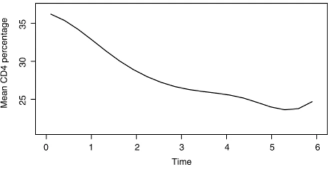
1. This indicates that age, and the quadratic

effects of age and preCD4 percentage have no significant impact on the mean CD4 percentage, which basically agrees with what was discovered by [34]. In addition, the curve of the estimated baseline function is show inFig. 1. FromFig. 1, we find that the mean baseline CD4 percentage decreases very quickly at the beginning of HIV infection, and the rate of decrease somewhat slows down four years after infection. This result is similar to what was discovered based on the varying coefficient models by [17,33].

5. Conclusion and discussion

We have proposed a variable selection procedure for the semiparametric varying coefficient partially linear model when the explanatory variables in the parametric and nonparametric components are subject to measurement errors. Our method

Fig. 1. Application to AIDS data. The regularized estimators for the mean CD4 percentageθ0(t), based on CLASSO.

extends the group lasso variable selection procedure to the semiparametric models. We have shown that the proposed method is consistent in variable selections, and the estimators of the regression coefficients have oracle property. Simulation studies indicate that the proposed method seems rather encouraging.

In this paper, although we assume that the covariates in the parametric and nonparametric components are all subject to measurement errors, it is not essential. Our variable selection procedure can easily extend the case that only some of the covariates are measured with errors, and the results in this paper still hold. However, the proofs of theoretical properties need slight modification.

To conclude this article, we would like to discuss some interesting topics for future study. Firstly, in this paper, we assume that the covariance matrix of measurement errors is known. However, it is usually unknown in many applications. If the covariance matrix is unknown, the variable selection procedure proposed by this paper will not work any more unless repeated measurements of the data are available. As a future research topic, it is interest to consider the variable selection for the semiparametric varying coefficient partially linear errors-in-variables models when the covariance matrix of measurement errors is unknown. Secondly, to avoid numerical instability, a threshold value is needed in the proposed iterative algorithm, which will potentially affect the degree of sparsity of the solution as well as the speed of convergence of our iterative algorithm. Then, how to give an optimal threshold value needs further investigation. In addition, how to extend the group LARS algorithm, proposed by [26] for parametric models, to the semiparametric models with measurement errors is another interesting topic of further research.

Acknowledgments

This research was supported by the National Natural Science Foundation of China (10871013), the Natural Science Foundation of Guangxi (2010GXNSFB013051), the Natural Science Foundation of Beijing (1102008), the Ph.D. Program Foundation of Ministry of China (20070005003), the Graduate Student Foundation of Hechi University (2008QS-N014), and the Funding Project for Academic Human Resources Development in Institutions of Higher Learning Under the Jurisdiction of Beijing Municipality (IHLB). The authors thank Drs Huang and Wu for allowing us to use the dataset ‘‘MACS Public Use Data Set Release PO4 (1984–1991)’’.

Appendix. Proof of theorems

For convenience and simplicity, letCdenote a positive constant that may be different at each appearance throughout this paper. Before we prove our main theorems, we list some regularity conditions that are used in this paper.

C1.

θ(

u

)

isrth continuously differentiable on

(

0

,

1

)

, wherer

>

1

/

2.

C2. The density function ofU, sayf

(

u

)

, is bounded away from 0 and infinity on

[

0

,

1

]

. Furthermore, we assume thatf

(

u

)

is continuously differentiable on

(

0

,

1

)

.

C3. LetΨ

(

u

)

=

E

{

X∗_Z∗T

|

_U

=

_u

}

_andΦ

(

_u

)

=

_E

{

_X∗_X∗T

|

_U

=

_u

}

_{. Then,Ψ}

(

_u

)

_andΦ

(

_u

)

_{arerth continuously differentiable} with respect tou. Furthermore, for givenu,Φ

(

u

)

is a positive definite matrix, and the eigenvalues ofΦ

(

u

)

are bounded. C4. Letc1

, . . . ,

cK be the interior knots of

[

0

,

1

]

. Furthermore, we letc0

=

0,cK+1

=

1,hi

=

ci

−

ci−1. Then, there exists a

constantC0such that

max

{

hi

}

/

min

{

hi

} ≤

C0

,

max

{|

hi+1

−

hi

|} =

o K−1

.

C5. Letan

=

maxk,l

{

λ

1k, λ2l

:

βl

0

6=

0

, γk

0

6=

0

}

, then

√

nan

→

0, asn

→ ∞

. C6. Letbn

=

mink,l

{

λ

1k, λ2l

:

βl

0

=

0

, γk

0

=

0

}

, then

√

nbn

→ ∞

, asn

→ ∞

.

These conditions are commonly adopted in the nonparametric literature and variable selection methodology. Conditions C1–C3 are similar to those used in [8,17,18]. Condition C4 implies thatc0

, . . . ,

cK+1 is aC0-quasi-uniform sequence of

partitions of

[

0

,

1

]

(see [36], p. 216). Conditions C5 and C6 are assumptions on the penalty function, which are similar to that used in [20,27].

Proof of Theorem 1. Let

δ

=

n−r/(2r+1),

β

=

β

₀

+

δα

₁,

γ

=

γ

₀

+

δα

₂and

α

=

(α

₁T

, α

T₂

)

T. For part (i), we first show that, for any given

ε >

0, there exists a large constantCsuch that

P

inf kαk=CQ

(γ , β) >

Q

(γ

0

, β

0

)

≥

1

−

ε.

(10) Let∆

(γ , β)

=

K−1

{

_Q

(γ , β)

−

_Q

(γ

0

, β

0

)

}

, then invoking

βl0

=

0,l

=

s

+

1

, . . . ,

qand

γk0

=

0,k

=

d

+

1

, . . . ,

p, we have

that ∆

(γ , β)

≥

1 K n

X

i=1

n

(

Yi

− ˜

WiT

γ

−

η

T i

β)

2

−

(

_Y i

− ˜

WiT

γ

0

−

η

iT

β

0

)

2

o

×

−

1 K n

X

i=1

(β

T_Σ νν

β

−

β

0TΣνν

β

0

)

+

(γ

TΩ

(

Ui

)γ

−

γ

0TΩ

(

Ui

)γ

0

)

+

n K s

X

l=1

λ

2l

|

βl

| −

λ

2l

|

βl0

|

+

n K d

X

k=1

λ

1k

k

γk

k

H

−

λ

1k

k

γk0

k

H

≡

I1

+

I2

+

I3

+

I4

.

Then, a simple calculation yields I1

=

−

2

δ

K n

X

i=1

(

X_iTR

(

Ui)

+

i

−

ϕ

_iT

γ

₀

−

ν

_iT

β

₀

)(

W_iT

α

2

+

ZiT

α

1

)

+

−

2

δ

K n

X

i=1

(

X_iTR

(

Ui)

+

i)(ϕ

_iT

α

₂

+

ν

T_i

α

₁

)

+

2

δ

K n

X

i=1

(ϕ

T i

γ

0

+

ν

iT

β

0

)(ϕ

iT

α

2

+

ν

iT

α

1

)

+

δ

2 K n

X

i=1

(

W_iT

α

2

+

ϕ

Ti

α

2

+

ZiT

α

1

+

ν

iT

α

1

)

2

≡

I11

+

I12

+

I13

+

I14

,

whereR

(

u

)

=

(

R1

(

u

), . . . ,

Rp(u

))

T,Rk(u

)

=

θk

0

(

u

)

−

B

(

u

)

T

γk

0,k

=

1

, . . . ,

p, and

ϕi

=

Ip

⊗

B

(

Ui)

·

υi

. From conditions C1, C4 and Corollary 6.21 in [36], we get that

k

Rk(

·

)

k =

O

(

K−r

).

(11)

Then, invoking condition C3, a simple calculation yields n

X

i=1

X_iTR

(

Ui)(W_iT

α

2

+

ZiT

α

1

)

=

Op(nK−r

k

α

k

).

(12)

In addition, notice thatE

{

i

−

ϕ

T

i

γ

0

−

ν

Ti

β

0

|

Zi

,

Xi,Ui

} =

0, we can prove that

1

√

n n

X

i=1

(i

−

ϕ

T_i

γ

₀

−

ν

_iT

β

₀

)(

W_iT

α

2

+

ZiT

α

1

)

=

Op(

k

α

k

).

Taking this together with(12), it is easy to show that I11

=

Op(

√

nK−1

δ)

k

α

k +

Op(nK−1−r

δ)

k

α

k =

Op(

k

α

k

).

(13) Similarly, we can prove thatI12

=

Op(

k

α

k

)

, and

I13

=

2

δ

K n

X

i=1

α

T 2

ϕiϕ

T i

γ

0

+

2

δ

K n

X

i=1

α

T 1

νiν

T i

β

0

+

op(

k

α

k

),

I14

=

δ

2 K n

X

i=1

(

W_iT

α

2

+

ZiT

α

1

)

2

+

δ

2 K n

X

i=1

(α

T 2

ϕiϕ

T i

α

2

+

α

T1

νiν

T i

α

1

)

+

op(

k

α

k

2

).

In addition, note that I2

=

−

2

δ

K n

X

i=1

(α

T 2Ω

(

Ui)γ0

+

α

1TΣνν

β

0

)

+

−

δ

2 K n

X

i=1

(α

T 2Ω

(

Ui)α2

+

α

1TΣνν

α

1

).

Then, we have I1

+

I2

=

δ

2 K n

X

i=1

(

W_iT

α

2

+

ZiT

α

1

)

2

+

δ

2 K n

X

i=1

α

T 2

(ϕiϕ

T i

−

Ω

(

Ui))α2

+

δ

2 K n

X

i=1

α

T 1

(νiν

T i

−

Σνν

)α

1

+

2

δ

K n

X

i=1

α

T 2

(ϕiϕ

Ti

−

Ω

(

Ui))γ0

+

2

δ

K n

X

i=1

α

T 1

(νiν

iT

−

Σνν

)β

0

+

Op(

k

α

k

)

+

op(

k

α

k

2

)

≡

J1

+

J2

+

J3

+

J4

+

J5

+

Op(

k

α

k

)

+

op(

k

α

k

2

).

InvokingE

(ϕi

ϕ

T_i

−

Ω

(

Ui))

=

0 andE

(νiν

_iT

−

Σ_νν

)

=

0, with the same arguments as in the proof of(13), we have that Js

=

Op(

√

nK−1

δ

2

)

k

α

k

2

=

_op(

k

α

k

2

),

_s

=

₂

,

_{3, andJ}

s

=

Op(

√

nK−1

δ)

k

α

k =

_op(

k

α

k

),

_s

=

₄

,

_{5. Furthermore, it is clear that}

J1

=

Op(nK−1

δ

2

)

k

α

k

2

=

Op(

k

α

k

2

).

Hence, by choosing a sufficiently largeC,J1dominates the other terms ofI1

+

I2uniformly in

k

α

k =

C. Next, we prove that

I3andI4are also dominated byJ1. By a simple calculation, we get that

I3

≤

snK−1

δ

an

k

α

k =

snr/(2r+1)an

k

α

k

.

Then, by condition C5, it is easy to show thatI3

=

op(

k

α

k

)

which is dominated byJ1uniformly in

k

α

k =

C. With the same

argument, we can prove thatI4is also dominated byJ1uniformly in

k

α

k =

C. Hence, by choosing a sufficiently largeC,(10)

holds. This implies, with probability at least 1

−

ε

, that there exists a local minimum in the ball

{

β

₀

+

δα

₁

: k

α

₁

k ≤

C

}

. Hence, there exists a local minimizer

β

ˆ

such that

k ˆ

β

−

β

₀

k =

Op(δ), which completes the proof of part (i).

Next, we prove part (ii). Note that

k ˆ

θk(

·

)

−

θk

₀

(

·

)

k

2

=

Z

1 0

n

ˆ

θk(

u

)

−

θk

₀

(

u

)

o

2 du

=

Z

1 0

B

(

u

)

T

γk

ˆ

−

B

(

u

)

T

γk

0

+

Rk0

(

u

)

2 du

≤

2

Z

1 0

B

(

u

)

T

γk

ˆ

−

B

(

u

)

T

γk

0 2 du

+

2

Z

1 0 Rk0

(

u

)

2du

=

2

(

γk

ˆ

−

γk

₀

)

TH

(

γk

ˆ

−

γk

₀

)

+

2

Z

1 0 Rk0

(

u

)

2du

.

With the same arguments as the proof of part (i), we can get that

k ˆ

γ

−

γ

₀

k =

Op(n−r/(2r+1)

)

_{. Then, invoking}

k

_H

k =

_O

(

₁

)

_{, a}

simple calculation yields

(

γk

ˆ

−

γk

₀

)

TH

(

γk

ˆ

−

γk

₀

)

=

Op

n2−r+2r1

.

(14)

In addition, it is easy to show that

Z

1 0 Rk0

(

u

)

2du

=

Op

n2−r+2r1

.

(15)

Invoking(14)and(15), we complete the proof of part (ii).

Proof of Theorem 2. We first prove part (i). ByTheorem 1, it is sufficient to show that, for any

γ

that satisfies

k

γ

−

γ

₀

k =

Op(n−r/(2r+1)

)

_,

βl

_{that satisfies}

|

βl

−

βl

0

| =

Op(n−r/(2r+1)

)

,l

=

1

, . . . ,

s, and some small

ε

=

Cn−r/(2r+1), whenn

→ ∞

, with

probability tending to 1 we have

∂

Q

(γ , β)

∂βl

>

0

,

for 0

< βl

< ε,

l

=

s

+

1

, . . . ,

q

,

(16) and

∂

Q

(γ , β)

∂βl

<

0

,

for

−

ε < βl

<

0

,

l

=

s

+

1

, . . . ,

q

.

(17)

Thus,(16)and(17)imply that the minimizer ofQ

(γ , β)

attains at

βl

=

0,l

=

s

+

1

, . . . ,

q. By a similar the proof of

Theorem 1, we have that

∂

Q

(γ , β)

∂βl

= −

2 n

X

i=1

ηil(

Yi

−

η

Ti

β

− ˜

W T i

γ )

−

2nΣνν,lβ

+

n

λ

2lsgn

(βl)

= −

2 n

X

i=1 Zil(Yi

− ˜

WiT

γ

−

Z T i

β

−

ν

T i

β)

−

2 n

X

i=1

νil(

Yi

− ˜

WiT

γ

−

Z T i

β)

−

2 n

X

i=1

(νilν

T i

β

−

Σνν,lβ)

+

n

λ

2lsgn

(βl)

=

n

λ

2l

n

sgn

(βl)

+

Op(λ₂−_l1n−2rr+1

)

o

.

By condition C6 and

λ

2ln r 2r+1

≥

bnn r

2r+1

→ ∞

,l

=

s

+

1

, . . . ,

q, we have that the sign of the derivation is completely determined by the sign of

βl

, then(16)and(17)hold. This completes the proof of part (i).

Applying similar techniques as in the analysis of part (i) in this theorem, we have, with probability tending to 1, that

ˆ

γk

=

0,k

=

d

+

1

, . . . ,

p. Then, invoking sup_u

k

B

(

u

)

k =

O

(

1

)

, the result of this theorem is immediately achieved from

ˆ

θk(

u

)

=

B

(

u

)

T

γk

ˆ

_.

Lemma 1. Suppose that the regularity conditions C1–C6 in theAppendixhold and the number of knotsK

=

O

(

n1/(2r+1)

)

. Then, 1 n n

X

i=1

˘

Z_i∗Z

˘

_i∗T

−→

P Σ

,

whereZ

˘

∗ i

=

Z ∗ i

−

ΨnTΦ −1 n W ∗ i,Φn

=

n−1

P

n i=1W ∗ i W ∗T i ,Ψn

=

n−1

P

n i=1W ∗ iZ ∗T i , and where P

−→

means the convergence in probability. Proof. LetW∗

=

(

W₁∗

, . . . ,

W_n∗

)

T,Z∗

=

(

Z₁∗

, . . . ,

Z_n∗

)

T andZ∗

=

(

_Z∗

−

_Γn)

+

_Γ n

≡

∆n

+

Γn, whereΓn

=

(

Ψ

(

U1

)

Φ

(

U1

)

−1X1∗

, . . . ,

Ψ

(

Un)Φ

(

Un) −1_X∗

n

)

T. Then a simple calculation yields 1 n n

X

i=1

˘

Z_i∗Z

˘

_i∗T

=

n−1Z∗T

(

I

−

PT

)(

I

−

P

)

Z∗

=

n−1

{

∆T_n∆_n

+

Γ_nT

(

I

−

PT

)(

I

−

P

)

Γn

+

∆Tn(I

−

PT

)(

I

−

P

)

Γn

+

Γ_nT

(

I

−

PT

)(

I

−

P

)

∆n

+

∆TnPTP∆n

}

,

(18)

whereP

=

W∗

(

_W∗T_W∗

)

−1_W∗T_{. By(11)and condition C3, there exists a matrixMsuch that}

k

_Γ

n

−

W∗M

k =

Op(n1/2K−r

)

. In addition, asPis a projection matrix, we have

k

(

I

−

P

)

Γn

k = k

Γn

−

W∗M

k + k

W∗M

−

PΓn

k

≤

2

k

Γ_n

−

W∗M

k =

Op(n1/2K−r

).

(19)

Furthermore, a simple calculation yieldsE

(

W∗T_∆

n

|

U1

, . . . ,

Un)

=

0. Then we have that

E

(

W∗T∆n)

=

0

,

and E

(

k

W∗T∆n

k

2

)

=

E n

X

i=1

k

W_i∗∆ni

k

2

!

=

Op(nK

),

where∆niis theith row of∆n. Hence

k

W∗T∆n

k =

Op(n1/2K1/2

)

. Then, we have

k

P∆n

k ≤ k

W∗

k k

W∗TW∗

kk

W∗T∆n

k

=

Op(n1/2K−1/2

)

Op(n−1K

)

Op(n1/2K1/2

)

=

Op(K

),

(20) and

k

(

I

−

P

)

∆n

k =

Op(n1/2

).

(21)

Hence, invoking(19)–(21), we have that all but the first term on the right-hand side of(18)areop(1

)

. Furthermore, by the law of large numbers, we can derive that the first term converges toΣin probability, so the result is proven as desired.

Proof of Theorem 3. ByTheorems 1and2, we know that, asn

→ ∞

, with probability tending to 1,Q

(γ , β)

attains the minimal value at

(

β

ˆ

∗T

,

₀

)

T_and

(

γ

ˆ

∗T

,

₀

)

T_{. LetQ}

1n(γ , β)

=

∂

Q

(γ , β)/∂β

∗andQ2n(γ , β)

=

∂

Q

(γ , β)/∂γ

∗, then,

(

β

ˆ

∗T

,

0

)

T

and

(

γ

ˆ

∗T

,

0

)

Tmust satisfy 1 nQ1n((

γ

ˆ

∗T

,

₀

)

T

, (

β

ˆ

∗T

,

₀

)

T

)

=

−

2 n n

X

i=1

η

∗ i

(

Yi

− ˜

Wi∗T

γ

ˆ

∗

−

η

∗T i

β

ˆ

∗

)

−

2Σ_νν∗

β

ˆ

∗

+

s

X

l=1

λ

2lsgn

(

βl)

ˆ

=

0

.

(22) 1 nQ2n((

γ

ˆ

∗T

,

₀

)

T

, (

β

ˆ

∗T

,

₀

)

T

)

=

−

2 n n

X

i=1

{ ˜

W_i∗

(

Yi

− ˜

Wi∗T

γ

ˆ

∗

−

η

∗T i

β

ˆ

∗

)

−

_Ω

(

Ui)

γ

ˆ

∗

} +

d

X

k=1

λ

1k H

γk

ˆ

k ˆ

γk

k

_H

=

0

.

(23)

ByTheorem 1and the condition C5, it is clear that s

X

l=1

λ

2lsgn

(

βl)

ˆ

=

op(

β

ˆ

∗

−

β

∗ 0

).

Then, combining the proofs ofTheorems 1and2, a simple calculation yields 1 n n

X

i=1 Z_i∗

{

Z_i∗T

(β

₀∗

− ˆ

β

∗

)

+

W_i∗T

(γ

₀∗

− ˆ

γ

∗

)

+

X_i∗TR∗

(

Ui)

+

i

} +

op(

β

ˆ

∗

−

β

₀∗

)

=

0

,

(24) 1 n n

X

i=1 W_i∗

{

Z_i∗T

(β

₀∗

− ˆ

β

∗

)

+

W_i∗T

(γ

₀∗

− ˆ

γ

∗

)

+

X_i∗TR∗

(

Ui)

+

i

} +

op(

γ

ˆ

∗

−

γ

₀∗

)

=

0

,

(25) whereX∗

i

=

(

Xi1

, . . . ,

Xid)TandR∗

(

u

)

=

(

R1

(

u

), . . . ,

Rd(u

))

T. Then, by(25), we have that

ˆ

γ

∗

−

γ

∗ 0

= [

Φn

+

op(1

)

]

−1

n

Ψn(β∗ 0

− ˆ

β

∗

)

+

Λn

o

,

whereΛn

=

n−1

P

n i=1W ∗ i

(

X ∗T i R ∗

(

Ui)

+

i)

. Substituting this into(24), and a simple calculation yields 1 n n

X

i=1 Z_i∗

{

Z_i∗T

−

W_i∗TΦ_n−1Ψn

}

(

β

ˆ

∗

−

β

0∗

)

+

op(

β

ˆ

∗

−

β

∗ 0

)

=

1 n n

X

i=1 Z_i∗

i

+

X_i∗TR∗

(

Ui)

−

W_i∗T

[

Φ_n−1

+

op(1

)

]

Λ_n

.

(26) Note that 1 n n

X

i=1 ΨT nΦ −1 n W ∗ i

{

Z ∗T i

−

W ∗T i Φ −1 n Ψn

} =

0

,

and 1 n n

X

i=1 ΨT nΦ −1 n W ∗ i

i

+

X_iTR

(

Ui)

−

W_i∗TΦ_n−1Λn

=

0

.

Then, by(26), it is easy to show that

(

1 n n

X

i=1

˘

Z_i∗Z

˘

_i∗T

+

op(1

)

)

√

n

(

β

ˆ

∗

−

β

₀∗

)

=

√

1 n n

X

i=1

˘

Z_i∗

i

+

√

1 n n

X

i=1

˘

Z_i∗W_i∗T

[

Φ_n−1

+

op(1

)

]

Λ_n

+

√

1 n n

X

i=1

˘

Z_i∗X_i∗TR∗

(

Ui

)

≡

∆₁

+

∆₂

+

∆₃

,

(27)

whereZ

˘

_i∗

=

Z_i∗

−

Ψ_nTΦ_n−1W_i∗. Using the similar proof ofLemma 1, we have that 1 n n

X

i=1

˘

Z_i∗Z

˘

_i∗T

2_i

−→

P

σ

2Σ

.

Hence by the Central Limits Theorem, we can obtain

∆1

L

−→

N

(

0

, σ

2Σ

).

(28)

In addition, note that

P

n i Z

˘

∗ iW

∗T

i

=

0, we have that∆2

=

0. Next, we prove∆3

P

−→

0. A simple calculation yields

∆3

=

1

√

n n

X

i=1

{

Z_i∗

−

E

(

Ψn)TE

(

Φn)−1W_i∗

}

X_i∗TR∗

(

Ui)

+

√

1 n n

X

i=1

{

E

(

Ψn)TE

(

Φn)−1

−

Ψ_nTΦ_n−1

}

W_i∗X_i∗TR∗

(

Ui)

≡

∆₃₁

+

∆₃₂

.

InvokingE

{[

Z∗ i

−

E

(

Ψn)TE

(

Φn) −1_W∗ i

]

W ∗ i

} =

0, we can prove 1

√

n n

X

i=1

{

Z_i∗

−

E

(

Ψn)TE

(

Φn)−1W_i∗

}

W_i∗T

=

Op(1

).

Taking this together with

k

B

(

·

)

k =

O

(

1

)

,

k

R

(

·

)

k =

o

(

1

)

andW∗

i

=

Ip

⊗

B

(

Ui)

·

Xi∗, it is clear that∆31

=

op(1

)

. Similarly, we

can prove that∆32

=

op(1

)

. Then, invoking(27),(28),Lemma 1, and using the Slutsky Theorem, we completes the proof of

References

[1] Q. Li, C.J. Huang, D. Li, T.T. Fu, Semiparametric smooth coefficient models, Journal of Business & Economic Statistics 20 (2002) 412–422. [2] W. Zhang, S.Y. Lee, X. Song, Local polynomial fitting in semivarying coefficient models, Journal of Multivariate Analysis 82 (2002) 166–188. [3] J.Q. Fan, T. Huang, Profile likelihood inference on semiparametric varying-coefficient partially linear models, Bernoulli 11 (2005) 1031–1057. [4] J.H. You, Y. Zhou, Empirical likelihood for semiparametric varying-coefficient partially linear regression models, Statistics & Probability Letters 76

(2006) 412–422.

[5] Z. Huang, R. Zhang, Empirical likelihood for nonparametric parts in semiparametric varying-coefficient partially linear models, Statistics & Probability Letters 79 (2009) 1798–1808.

[6] R. Li, H. Liang, Variable selection in semiparametric regression modeling, The Annals of Statistics 36 (2008) 261–286.

[7] J.Q. Fan, R. Li, Variable selection via nonconcave penalized likelihood and its oracle properties, Journal of the American Statistical Association 96 (2001) 1348–1360.

[8] H.J. Wang, Z. Zhu, J. Zhou, Quantile regression in partially linear varying coefficient models, The Annals of Statistics 37 (2009) 3841–3866. [9] H.J. Cui, S.X. Chen, Empirical likelihood confidence region for parameter in the errors-in-variable models, Journal of Multivariate Analysis 84 (2003)

101–115.

[10] C.L. Cheng, J.V. Ness, Statistical Regression with Measurement Error, Arnold, London, 1999. [11] W.A. Fuller, Measurement Error Models, Wiley, New York, 1987.

[12] H. Cui, R. Li, On parameter estimation for semi-linear errors-in-variables models, Journal of Multivariate Analysis 64 (1998) 1–24.

[13] H. Liang, W. Härdle, R.J. Carroll, Estimation in a semiparametric partially linear errors-in-variables model, The Annals of Statistics 27 (1999) 1519–1535. [14] H. Liang, R. Li, Variable selection for partially linear models with measurement errors, Journal of the American Statistical Association 104 (2009)

234–248.

[15] J. You, Y. Zhou, G. Chen, Corrected local polynomial estimation in varying-coefficient models with measurement errors, The Canadion Journal of Statistics 34 (2006) 391–410.

[16] L. Li, T. Greene, Varying coefficients model with measurement error, Biometrics 64 (2008) 519–526.

[17] L.G. Xue, L.X. Zhu, Empirical likelihood for a varying coefficient model with longitudinal data, Journal of the American Statistical Association 102 (2007) 642–652.

[18] Q.G. Tang, L.S. Cheng,M-estimation and B-spline approximation for varying coefficient models with longitudinal data, Journal of Nonparametric Statistics 20 (2008) 611–625.

[19] L. Wang, H. Li, J.Z. Huang, Variable selection in nonparametric varying-coeddicient models for analysis of repeated measurements, Journal of the American Statistical Association 103 (2008) 1556–1569.

[20] H.S. Wang, Y.C. Xia, Shrinkage estimation of the varying coefficient model, Journal of the American Statistical Association 104 (2009) 747–757. [21] C. Leng, A simple approach for varying-coefficient model selection, Journal of Statistical Planning and Inference 139 (2009) 2138–2146.

[22] J. You, G. Chen, Estimation of a semiparametric varying-coefficient partially linear errors-in-variables model, Journal of Multivariate Analysis 97 (2006) 324–341.

[23] X. Hu, Z. Wang, Z. Zhao, Empirical likelihood for semiparametric varying-coefficient partially linear errors-in-variables models, Statistics & Probability Letters 79 (2009) 1044–1052.

[24] P.X. Zhao, L.G. Xue, Empirical likelihood inferences for semiparametric varying-coefficient partially linear errors-in-variables models with longitudinal data, Journal of Nonparametric Statistics 21 (2009) 907–923.

[25] Y. Zhou, H. Liang, Statistical inference for semiparametric varying-coefficient partially linear models with error-prone linear covariates, The Annals of Statistics 37 (2009) 427–458.

[26] M. Yuan, Y. Lin, Model selection and estimation in regression with grouped variables, Journal of the Royal Statistical Society: Series B 68 (2006) 49–67. [27] H.S. Wang, C. Leng, A note on adaptive group lasso, Computational Statistics and Data Analysis 52 (2008) 5277–5286.

[28] P.X. Zhao, L.G. Xue, Variable selection for semiparametric varying coefficient partially linear models, Statistics & Probability Letters 79 (2009) 2148–2157.

[29] C.J. Stone, Optimal global rates of convergence for nonparametric regression, The Annals of Statistics 10 (1982) 1348–1360. [30] W.J. Fu, Penalized regression: the bridge versus the LASSO, Journal of Computational and Graphical Statistics 7 (1998) 397–416. [31] B. Efron, T. Hastie, I. Johnstone, R. Tibshirani, Least angle regression, The Annals of Statistics 32 (2004) 407–489.

[32] H. Zou, The adaptive lasso and its oracle properties, Journal of the American Statistical Association 101 (2006) 1418–1429.

[33] J.Z. Huang, C.O. Wu, L. Zhou, Varying-coefficient models and basis function approximations for the analysis of repeated measurements, Biometrika 89 (2002) 111–128.

[34] J.Q. Fan, R. Li, New estimation and model selection procedures for semiparametric modeling in longitudinal data analysis, Journal of the American Statistical Association 99 (2004) 710–723.

[35] L.G. Xue, L.X. Zhu, Empirical likelihood semiparametric regression analysis for longitudinal data, Biometrika 94 (2007) 921–937. [36] L.L. Schumaker, Spline Functions, Wiley, New York, 1981.