Online Client-Server Load Balancing Without
Global Information
∗
Baruch Awerbuch† Mohammad T. Hajiaghayi‡ Robert Kleinberg‡ § ¶ Tom Leighton‡§
Abstract
We consider distributed online algorithms for maximizing throughput in a net-work of clients and servers, modeled as a bipartite graph. Unlike most prior net-work on online load balancing, we do not assume centralized control and seek algorithms and lower bounds for decentralized algorithms in which each participant has only local knowledge about the state of itself and its neighbors. Our problem can be seen as analogous to the recent work on oblivious routing in [8, 14, 20], but with the objective of maximizing throughput rather than minimizing congestion. In con-trast to that work, we prove a strong lower bound (polynomial inn, the size of the graph) on the competitive ratio of any oblivious algorithm. This is accompanied by simple algorithms achieving upper bounds which are tight in terms of k, the maximum throughput achievable by an omniscient algorithm. Finally, we examine a restricted model in which clients, upon becoming active, must remain so for at leastlog(n)time steps. In contrast to the primarily negative results in the oblivi-ous case, here we present an algorithm which is constant-competitive. Our lower bounds justify the intuition, implicit in earlier work on the subject [2], that some such restriction (i.e. requiring some stability in the demand pattern over time) is necessary in order to achieve a constant — or even polylogarithmic — competitive ratio.
1
Introduction
We consider distributed online algorithms for maximizing throughput in a network of clients and servers, modeled as a bipartite graphG= (VL, VR, E)withVLrepresenting the clients,VRrepresenting the servers, andErepresenting the client-server assignments which are considered admissible, e.g. because of proximity constraints. Motivated by Internet load-balancing applications, such as load-balancing HTTP connections in
∗A preliminary version of this paper appeared in Proceedings of the 16th Annual ACM-SIAM Sympo-sium on Discrete Algorithms, 2005.
†Center for Networking and Distributed Systems, Johns Hopkins University, U.S.A.,
‡Department of Mathematics and Computer Science and Artificial Intelligence Laboratory,
Mas-sachusetts Institute of Technology, 200 Technology Square, Cambridge, MA 02139, U.S.A.,
{hajiagha,rdk,ftl}@theory.lcs.mit.edu
§Akamai Technologies, 8 Cambridge Center, Cambridge, MA 02139, U.S.A. ¶Supported by a Fannie and John Hertz Foundation Fellowship.
a content delivery network, we consider the case where client-server connections are extremely short-lived (lasting for only one unit of time) and it is impossible to get an instantaneous snapshot of the demand pattern. Our focus is on distributed algorithms in which clients must make decisions knowing nothing about the current demand pattern other than their own demand, and servers must make decisions knowing nothing other than what they learn from their adjacent clients. (We also assume that servers may report their load to the adjacent clients at the end of a round, though this is not necessarily predictive of their load in future rounds.) This emphasis on distributed algorithms with a very limited amount of communication is what distinguishes the present paper from most of the previous work on online load balancing.
Our model of online load-balancing is completely stateless, since client-server con-nections last for only one unit of time and the demand pattern may be completely dif-ferent in the next round. Thus, if the demand pattern is allowed to vary arbitrarily and adversarially over time, an online algorithm’s competitive ratio over a sequence of T
steps will generally be no better than its competitive ratio in the caseT = 1, i.e. a one-shot game between the algorithm and the adversary. It may seem hopeless to achieve non-trivial upper bounds on competitive ratio in such a one-shot game, since the al-gorithm has no time to learn any information about the demand pattern before making its decisions. However, the recent result of R¨acke [20] (and its subsequent construc-tive results by Harrelson, Hildrum, and Rao [14] and Bienkowski, Korzeniowski and R¨acke [8]) on oblivious routing in undirected networks demonstrate that it is sometimes possible to achieve surprisingly strong upper bounds for such “one-shot” load balancing problems. Specifically, for a multicommodity flow problem in an undirected graph G, it is possible for each commodity to choose a flow without knowing the demand of any
other commodity, in such a way that the maximum edge congestion in G is within a
O(log2nlog logn) factor of that of the congestion-minimizing flow for the given de-mand pattern.
Much of the present paper is devoted to analyzing the analogous question for client-server load-balancing. While it is possible to achieve competitive ratios significantly better than the trivial O(n) bound for this problem, we show that it is impossible to achieve apolylog(n)competitive ratio. A comparably strong lower bound for oblivious routing in bipartite directed graphs was established using a simple construction in [6]. Our lower bound requires a significantly more sophisticated construction because we seek a lower bound on competitive ratio for throughput rather than edge congestion. This is the first polynomial lower bound on throughput for oblivious routing.
As a counterpoint to these primarily negative results, we consider a restricted ad-versarial model in which clients have{0,1}-valued demands (i.e. they are either active or inactive), and a client who becomes active must remain active for at least r rounds thereafter. In this environment, we present an algorithm whose competitive ratio is
O(∆6/r),where∆is an upper bound (known to all parties) on the degree of any client. In particular, the algorithm achieves a constant competitive ratio when r = Ω(log ∆).
Our algorithm is structurally similar to the concurrent routing algorithm of [2], with two important differences: the latter algorithm assumes that clients are not entering and leaving the system over time, and it requires the clients to gradually increase their flow until eventually reaching the desired level of throughput. Our algorithm permits clients to become active and inactive over time (provided that a client, upon becoming active, remains active for the nextr steps), and it permits them to route their full demand in each round in which they are active (though the demand may not be satisfied, if it is sent to a congested server).
All of the algorithms presented in this paper are very easy to implement, requiring straightforward decision-making and communication protocols on the part of clients and servers. Some of the lower bound proofs, on the other hand, are relatively sophisticated. We show that oblivious algorithms for throughput maximization can be obstructed by the presence of substructures in the bipartite graph which we call γ-focal matchings. The task of proving competitive-ratio lower bounds is thereby reduced to a combinato-rial problem of packing as manyγ-focal matchings as possible into a bipartite graph of sizen. Our construction of such graphs involves an interesting mixture of combinato-rial, algebraic, and probabilistic techniques. These lower bound techniques constitute one of main contributions of this paper, and we believe it may be interesting to consider whether they can be used to obtain lower bounds for other problems.
2
Related work
Recall that this paper considers load balancing for a client-server model which has two essential characteristics. The first one is that our system is fully dynamic and the input can change drastically from one time period to the next. The second one is that there is no central “dispatcher” in the system that could communicate the result of the maximum matching computation to the clients, thus guiding their routing decisions. Indeed, the interplay of these two aspects plays an important role in this paper, since otherwise there are many algorithms in the literature for models possessing only one of these characteristics. Below, we review some of these results.
2.1
Centralized control
Finding a maximum matching, or its generalization to maximum flow, is one of the clas-sical problems in combinatorial optimization. The fastest known sequential algorithm for the problem has running time close toO(|E||V|)[12]. For the more general prob-lem of solving a positive linear program to within a(1 +)factor of optimality, Plotkin, Shmoys, and Tardos [19] present a sequential algorithm which repeatedly identifies a globally minimum weight path, and pushes more flow along that path. The algorithm of Plotkin et al. is further improved by Garg and Konemann [10], who give faster and simpler primal-dual algorithms for multicommodity flow and other fractional packing
problem with the same approximation factor(1 +). In addition, several (determinis-tic and randomized) parallel algorithms for maximum bipartite matching and maximum flow have been proposed (see e.g. [9, 12, 15]). Although these algorithms have effi-cient implementations, they are all centralized algorithms and require global kowledge of the demand pattern and global coordination, which make them unsuitable for fast distributed implementation with local information.
2.2
Distributed control with persistent demands
Routing and admission control. Assuming that the demand pattern remains stable
for at leastΩ(logn)rounds at a time, a distributed routing and flow control algorithm with a global objective function has been given by Awerbuch and Azar [2]. This work is based on fundamental results from competitive analysis [1, 3] and assumes clients can gradually increase their flow; while the flow is still small it could for example be buffered at the client. In this case, under the assumption that there is a small number of routing paths, they provide anO(logn)-competitive algorithm for the routing problem, which takes a polylogarithmic number of rounds to converge. Awerbuch and Leighton [4, 5] have suggested general methods for distributed routing and admission control that use a polynomial amount of buffer space. Our lower bounds demonstrate that at least one of these two assumptions — persistence of demands over time, or the ability to buffer packets — is really required in order to achieve a polylogarithmic competitive ratio.
Distributed admission control alone. For the distributed admission control problem
(in which clients do not choose a server or routing path, but only their sending rate) Papadimitriou and Yannakakis [18] initiated the study of flow control using distributed routers based only on local information. More precisely, they presented a framework for solving positive linear programs by distributed agents. Luby and Nisan [16], Bar-tal, Byers and Raz [7] and finally Garg and Young [11] obtained(1 +)-competitive algorithms converging in a polylogarithmic number of rounds.
Even though all of these results are distributed, they converge to their final solu-tion in a polylogarithmic number of rounds, which makes them unsuitable for our fully dynamic client-server model.
2.3
Distributed control without persistence of demands
One possible approach to distributed load-balancing is to use an “oblivious” solution. Such an oblivious algorithm exists for the congestion minimization problem in undi-rected edge-capacitated graphs (see [20] and its subsequent improvement by Harrelson, Hildrum, and Rao [14]) and for directed and node-capacitated graphs [13]. No such so-lution exists for the throughput problem, though R¨acke and Rosen (independently and concurrently with our work) gave a distributed online call control algorithm which is
closely related to oblivious throughput maximization in undirected graphs [21]. One of the main results in our paper establishes nearly tight upper and lower bounds on the performance of oblivious routing schemes in directed bipartite graphs, in terms of throughput. The performance gap between the optimal and oblivious solution is poly-nomial; our lower bounds show that this gap is inherent.
3
Formal model and statement of results
Our graph terminology is as follows. All the graphs in this paper are directed bipartite graphs without multiple edges. For such a graph G = (VL, VR, E), we will refer to elements of VL as clients and elements of VR as servers. The number of clients is denoted byn, the number of servers bym. The edges ofE are directed from clients to servers. For a vertex setS ⊆ VL∪VR we denote the set of adjacent vertices byΓ(S), the set of outgoing edges byδ+(S), and the set of incoming edges byδ−(S). When S
is a singleton set{v}, these will be abbreviated to Γ(v), δ+(v), δ−(v). The degree of a
vertexv will be denoted byd(v).
The prototypical problem we will analyze is the following online throughput max-imization problem. In each time stept (1 ≤ t ≤ T), an adversary designates a setSt of clients, called the active clients. Each active client i generates a request and must choose a (possibly random) adjacent server to which it will send this request, without knowing which other clients are active. Each server that receives one or more requests in roundtmay choose to satisfy any one of them. The goal is to maximize the expected number of satisfied requests, called the throughput. The algorithm is judged according to its competitive ratio, i.e. the ratio of its throughput to that of the omniscient algorithm which chooses a throughput-maximizing assignment in each period.
When the problem is posed in this form, its online nature is essentially irrelevant. This is because any algorithm achieving the optimum competitive ratio in theT = 1case also achieves the optimum competitive ratio in the case of generalT, by simply ignoring past history and treating each round as if it were the first round. For this reason, we will focus most of our attention on the T = 1case, which we call the one-shot model. We will use the letterk to denote the throughput of the optimal assignment, i.e. the size of a maximum matching from the active clients toVR.
The following variants of the problem are also of interest.
Multicast model In contrast to the unicast model described above, we may consider a
model in which a client may send its request to any subset of the adjacent servers. A server receiving one or more requests may choose to satisfy any one of them, but it must make this choice without any knowledge about the set of active clients other than the information contained in the requests it received. The throughput is defined as the number of distinct clients whose requests are satisfied, i.e. a client whose request is satisfied by two or more servers still contributes only1 to the throughput.
Fractional assignments Instead of requiring each active client i to choose one of its adjacent servers, it may choose a fractional load distribution among its outgoing edges. In other words, each client chooses a functionfi : δ+(i) →[0,1] satisfy-ingP
e∈δ+(i)f(e)≤1. As always, clientimust specifyfiwithout knowing which
other clients are inS. The load on a serverj, denoted by`(j), is equal to the total load on all incoming edges. The throughput is defined byP
j∈VRmin{1, `(j)}.
Restricted adversary In the restricted-adversary model, we assume that the setsSt of active clients satisfy the following constraint: every client, upon becoming active, must remain active for the nextrrounds. In other words, ifi∈St then there exist
t0, t1 such thatt0 ≤ t ≤t1, t1−t0 ≥ r, andi ∈ St0 fort0 ≤ t0 ≤ t1. (We callr
the minimum activity period.) We also assume that servers may report their load and capacity to the adjacent clients at the end of each round.
In proving lower bounds in this paper, we will assume that the structure of the entire graph Gis known to all clients and servers, and that they have access to an unlimited supply of shared random bits. In contrast, our upper bounds will be based on algorithms which require much less knowledge on the part of the participants: each vertex need only know which vertices are adjacent to it. (In Section 7 we must also assume that they share a common estimate of the maximum client degree,∆.)
The following theorems summarize our main results.
Theorem 1. In the unicast one-shot model, there is an algorithm whose competitive
ratio isO(√k), and this bound is tight in terms ofk, even if the algorithm is randomized and is allowed to use fractional assignments. In terms ofn, the competitive ratio of any such algorithm isΩ(n0.103).
Theorem 2. In the multicast one-shot model, there is an algorithm whose competitive
ratio is O(k1/3), provided that the servers know the degree of their adjacent clients or that the clients can communicate this information in their request headers. This bound is tight in terms of k, even if the clients are allowed to put an arbitrary amount of information in the request header. In terms ofn, the competitive ratio of any such algorithm isΩ(n0.069).
Theorem 3. In the restricted adversary model with fractional assignments and with
minimum activity periodr, if the clients know the value ofras well as an upper bound
∆on the maximum degree of any client, then there is an algorithm whose competitive ratio isO(∆6/r). In particular, ifr= Ω(log ∆),the competitive ratio is constant.
It is worth mentioning that the proofs of Theorems 1 and 2 also establish tight bounds on the optimal competitive ratio in terms of m, the number of servers. The optimal competitive ratio is θ(m1/2)in the unicast model andθ(m1/3) in the multicast model.
4
Lower bounds for the one-shot model
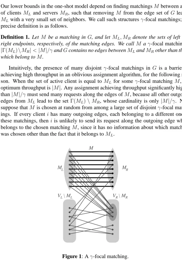
Our lower bounds in the one-shot model depend on finding matchingsM between a set of clients ML and serversMR, such that removingM from the edge set of G leaves
ML with a very small set of neighbors. We call such structuresγ-focal matchings; the precise definition is as follows.
Definition 1. Let M be a matching in G, and let ML, MR denote the sets of left and
right endpoints, respectively, of the matching edges. We callM aγ-focal matching if
|Γ(ML)\MR|<|M|/γandGcontains no edges betweenMLandMRother than those
which belong toM.
Intuitively, the presence of many disjoint γ-focal matchings in G is a barrier to achieving high throughput in an oblivious assignment algorithm, for the following rea-son. When the set of active client is equal to ML for some γ-focal matching M, the optimum throughput is|M|. Any assignment achieving throughput significantly higher than|M|/γ must send many requests along the edges ofM, because all other outgoing edges from ML lead to the set Γ(ML)\MR, whose cardinality is only |M|/γ. Now suppose thatM is chosen at random from among a large set of disjointγ-focal match-ings. If every client i has many outgoing edges, each belonging to a different one of these matchings, then i is unlikely to send its request along the outgoing edge which belongs to the chosen matchingM, since it has no information about which matching was chosen other than the fact that it belongs toML.
M M M V \ M V \ M L R L L R R
4.1
Unicast lower bounds
LetAdenote the set of all fractional assignments inG, i.e.
A={f : E →[0,1]| ∀i∈VL
X
j∈Γ(i)
f(i, j) = 1}.
A set S of active clients may be represented by a functionD : VL → {0,1}mapping
S to 1 and VL\S to 0; we call this the demand pattern associated with S. Given a fractional assignmentf, define the load on serverj by
`(j) = X
i∈Γ(j)
f(i, j)D(i)
and the throughput off by
θ(f) = X
j∈VR
min{`(j),1}.
We may think of a randomized assignment algorithm in the one-shot model as comput-ing a functionA : {0,1}VL
×X → A, whereXis a probability space encapsulating all the random bits (both shared and private) which the parties may use in their decision-making. The fact that the assignment is oblivious (i.e. that clients must choose their own assignment without knowing which other clients are active) is captured by the fol-lowing constraint: in the fractional assignment f = A(D, x), for any edge (i, j), the value of f(i, j)may only depend onD(i)andx. In other words, iff0 = A(D0, x)and
D0(i) =D(i), thenf0(i, j) =f(i, j).
Theorem 4. Let Gbe a bipartite graph which is (dL, dR)-biregular, i.e. everyi ∈ VL
has degreedL and everyj ∈VR has degreedR. Assume all servers have unit capacity.
If the edge set of G can be partitioned intoγ-focal matchings of equal size, then the competitive ratio of any oblivious randomized fractional assignment algorithm forGis at least 12min{dL, γ}.
Proof. Let A be any oblivious randomized fractional assignment algorithm, and let
M(1), . . . , M(s) be a partition ofE into γ-focal matchings of equal size k. Note that
the number of edges satisfiessk =|E|=dLn,whence
n s =
k dL
.
Let the demand patternD : VL→ {0,1}be defined by selecting a matchingM =M(r) uniformly at random from{M(1), . . . , M(s)}, independently of the algorithm’s random
seed x ∈ X, and settingD(i) = 1 if i ∈ ML, 0 otherwise. The throughput of the assignmentf =A(D, x)satisfies θ(f) = X j∈MR min{`(j),1}+ X j∈Γ(ML)\MR min{`(j),1} ≤ X j∈MR `(j) + X j∈Γ(ML)\MR 1 ≤ X e∈M f(e) +k/γ.
LetD∗ denote the demand pattern in which all clients are active, i.e.D∗(i) = 1∀i, and
letf∗ = A(D∗, x). By the definition of “oblivious,” we have thatf(i, j) = f∗(i, j)for
alli∈ML. Hence
θ(f)≤k/γ+X
e∈M
f∗(e).
Now let’s take the expectation over the random choice ofxandM.
E[θ(f)] ≤ k γ + X e∈E Pr(e ∈M)E[f∗(e)] = k γ + 1 s X e∈E E[f∗(e)] = k γ + 1 sE X i∈VL X e∈δ+(i) f∗(e) ≤ γk + n s = k γ + k dL ≤ 2k min{dL, γ} .
The optimal assignment sends the k requests along the edges of M, thus achieving throughputk. Hence the competitive ratio ofAis at least 12min{dL, γ},as claimed.
Theorem 5. There exists a bipartite graph G such that the competitive ratio of any oblivious randomized fractional assignment algorithm forGis at least√k/2, where k
is the maximum throughput achievable in the given problem instance.
Proof. The graphGis defined as follows. Given a positive integerd, letVR be the set
{1,2, . . . , d2},and letV
Lbe the set of alld-element subsets ofVR.Each such seti∈VL is joined by an edge to each of its elements j ∈ VR. Gis a biregular bipartite graph, withdL=danddR= d
2−1
d−1
.
For each (d −1)-element subsetS ⊆ VR, let M(S) be the matching containing, for each j ∈ VR\ S,an edge from i = S ∪ {j} to j. Each such matching has size
d2 −d + 1, and each edge (i, j) ∈ E belongs to exactly one such matching M(S).
We claim that each matchingM = M(S)is ad-focal matching. We have MR =
VR \S, and each i ∈ MLhas one edge joining it toMR(namely, the matching edge) andd−1edges joining it toS. ThusGcontains no edges between MLandMR other than the matching edges, and
|Γ(ML)\MR|<|M|/d,
because the left side is equal tod−1while the right side is equal tod−1 + 1/d. Applying Theorem 4, we find that the competitive ratio of any oblivious randomized fractional assignment algorithm is at least d/2, which is greater than √k/2 because
k =d2−d+ 1.
Note that the proof of Theorem 5 also gives a lower bound of√m/2wheremis the number of servers. (We will see later that this bound is tight, up to a constant factor, in terms of m.) However the number of clients in this example, n, is equal to dd2, so the competitive-ratio lower bound ofd/2only translates into a very weak lower bound ofΩ(logn/log logn) in terms ofn. The following theorem demonstrates that a much stronger lower bound is possible.
Theorem 6. There exists a bipartite graph G such that the competitive ratio of any oblivious randomized fractional assignment algorithm forGisΩ(n0.103).
Proof. The construction of the graphGin this case is quite complicated. For a positive integer d, let X be the ring (F2)d, i.e. the cartesian product of d copies of the field
F2 = {0,1}. Considering X as a vector space over F2, let Y be a linear subspace of
dimension bd. (We will optimize the value of the parameter b < 1 later on.) Let Z
denote the set of all z in X such that zy is non-zero for all non-zero y ∈ Y. (If we identify elements of X with subsets of {1,2, . . . , d}, then the non-zero elements ofY
constitute a set system and Z consists of all hitting sets for this set system.) We will want the complement, X \Z, to be as small as possible. Here is a calculation which bounds the expected size ofX\ZwhenY is a random linear subspace of dimensionbd. For any non-zeroy ∈X, the probability that it belongs toY is2(b−1)d, and the number ofz such thatzy = 0is2d−wt(y), wherewt(y)denotes the Hamming weight ofy. This
means that an upper bound for the expected size ofX\Z is given by:
X y∈X, y6=0 2(b−1)d2d−wt(y) = 2bd X y∈X, y6=0 2−wt(y) = 2bd d X j=1 d j 2−j = 2bd (3/2)d−1 < (3·2b−1)d
Henceforth we assume that we have chosen a specific linear subspace Y such that the cardinality ofX \Z is at most(3·2b−1)d. Later on, when we specify the value ofb, it will be the case that3·2b−1 =√3·(1 +o(1)), so the fraction of elements ofXwhich
are not contained inZis exponentially small ind. The bipartite graphGis defined as follows. We put
VL = X×Z
VR = X
E = {((xL, zL), xR)|xR−xL=yzLfor somey∈Y}.
By abuse of notation, we will write an edge e with left endpoint (xL, zL) and right endpointxRas an ordered triplee= (xL, zL, xR). Note that ifxR−xL =yzLfor some
y ∈ Y, then this y is actually unique. (If yzL = y0zL, then (y− y0)zL = 0. Since
y−y0 ∈Y andz ∈Z, this impliesy−y0 = 0.) We will refer to this unique value ofy
as the type of edgee= (xL, zL, xR).
We have seen that each(xL, zL) ∈ VL has exactly|Y|outgoing edges, one of each type y ∈ Y. Similarly, each xR ∈ VR has exactly |Y × Z| incoming edges. Given
(y, z) ∈ Y ×Z, one may easily verify that there is one and only one edge of type y
joiningX× {z}toxR, namely the edgee= (xR−yz, z, xR). We have thus established thatGis(2bd,2bd· |Z|)-biregular.
We must now specify a partition of the edge set intoγ-focal matchings of equal size. For each pair(x, y)wherex∈X,y∈Y, let
M(x, y) ={(x+ ((1−y)z), z, x+z)|z ∈Z}.
where “1” denotes the vector(1,1,1, . . . ,1)∈X. Note that(x+ ((1−y)z), z, x+z)
is a valid edge of typeyinG, because x+z =x+ 1·z = x+ ((1−y)z) +yz.The matchings M(x, y) each have size|Z|. To see that every edge belongs to exactly one such matching, observe that ife= (xL, zL, xR)withxR−xL =yzL, thenebelongs to
M(xR−zL, y). There can be no otherM(x0, y0)containinge, sincey0 must equal the type ofeandx0 must equalx
R−zLin order foreto belong toM(x0, y0).
Next, we wish to see that each such matchingM = M(x, y)is γ-focal for a rea-sonably large (i.e. exponential ind) value ofγ. To do so, we will first show that every edge between ML and the setMR = x+Z = {x+z | z ∈ Z} belongs to M. Let
e = (xL, zL, xR) be such an edge, with xR −xL = y0zL for some y0 ∈ Y. Since
(xL, zL)∈ML, we havexL=x+ (1−y)zL,whencexR =x+ (1 +y0−y)zL. Ify0 =y thene∈M. Ify0 6=y, then we use the fact that every elementwof the ringXsatisfies
w(1−w) = 0.Applying this withw=y−y0, we see that(y−y0)(1 +y0−y)z
L = 0. Asy−y0 is a non-zero element ofY, we may conclude that(1 +y0−y)z
L6∈Z, whence
xR 6∈x+Z. Finally, observe that
Recalling that|M| =|Z|= (1−o(1))2d,we see thatM isγ-focal with
γ = (1−o(1)) 22−b/3d
.
Applying Theorem 4, we find that no oblivious randomized fractional assignment algorithm achieves a competitive ratio better than
1 2min{dL, γ}= 1 2min n 2bd, 22−b/3d (1−o(1))o.
This approximately maximized when 2b = 22−b/3, i.e. when b = 1− 1
2log2(3) =
0.2075. . .(Of course, b must be rounded to the nearest multiple of1/d, since bd, the dimension of the vector space Y, must be an integer.) Recalling thatn = |X ×Z| <
22d, we see that the lower bound of Ω(2bd) on competitive ratio may be expressed as
Ω(nb/2) = Ω(n0.103).
4.2
Multicast lower bounds
Proving lower bounds in the multicast model is slightly more difficult than in the uni-cast model, because clients may broaduni-cast their request to every adjacent server if they wish. If the set of active clients is equal toMLfor someγ-focal matchingM, and each client chooses to broadcast its request to all adjacent servers, then each server in MR will receive exactly one request and will satisfy it, leading to a throughput of|M|, the optimum throughput for the designated set of active clients. Nevertheless, it is possible to use γ-focal matchings to prove lower bounds in the multicast model, by combining them with another device which we call a smokescreen. A smokescreen is simply a random set of clients whose size is small relative to the size of the matching, and whose purpose is to confuse the servers in MR by making it difficult for them to distinguish which incoming request is coming fromML.
We will begin by formalizing the class of protocols which we will be considering. We will assume once again that there is a probability spaceXencapsulating the random bits (both shared and private) available to the parties in their computation. There is also a (not necessarily finite) message spaceMSGencapsulating all the messages that clients
may send to servers. A protocol is specified by a communication function
Ai :{0,1} ×X →MSGd(i) for each clientiand a decision function
Bj :MSGd(j)×X →Γ(j)
for each serverj. The value ofAi(D, x)specifies the d(i)-tuple of messages whichi will send on its outgoing edges if its demand isDand the random seed isx. The value of Bj(m1, m2, . . . , md(j), x)specifies which client’s request will be served by j if the
random seed is x and j receives messages m1, m2, . . . , md(j) on its incoming edges.
We will call such a protocol {Ai, Bj} an oblivious assignment protocol for G in the
multicast model.
Without loss of generality we may assume thatMSG={0,1}and that each
commu-nication functionAi is simply the functionAi(D, x) = D. In other words, each client simply informs all adjacent servers whether it is active or not. This assumption is with-out loss of generality because for any other protocol Pˆ = {Aˆi,Bˆj}, we can construct a protocol P = {Ai, Bj} with Ai defined as above, and with Bj defined as follows. For each client i ∈ Γ(j), Bj(m1, . . . , md(j), x)simulates Aˆi(mi, x)to determine what message mˆi would have been sent fromi toj under the protocolP, and it then com-putesBˆj( ˆm1, . . . ,mˆd(j), x)to determine what request it would have satisfied. This new
protocolP has precisely the same outcome asPˆ.
Based on this reduction, we will assume from now on that each server’s decision function is a mapping Bj : {0,1}Γ(j) ×X → Γ(j) which chooses, for each subset
S ⊆ Γ(j), a random elementBj(S, x) ∈ Γ(j)determined by the random seedx. The notion that servers have difficulty distinguishing elements of ML from elements of the smokescreen is captured by the following lemma.
Lemma 1. Let Γ be a set of d elements, and consider any function B : 2Γ → Γ. Suppose a random elementi∈ Γis sampled according to the uniform distribution, and a random set S ⊆ Γ\ {i} is sampled by choosing each element independently with probabilityp. ThenPr(B(S∪ {i}) =i) =O1
pd
.
Proof. For any non-empty setT ⊆Γof cardinalityt, we have
Pr(B(T) =ikS∪ {i}=T) =
1
t ifB(T)∈T
0 otherwise.
This is obvious ifB(T)6∈ T. AssumingB(T)∈ T, it holds because for every element
i0 ∈T, Pr(i=i0 ∧ S =T \ {i0}) = 1 d ·p t−1 ·(1−p)d−t.
Denoting this probability byp0, we have
Pr(S∪ {i}=T) = X i0∈T Pr(i=i0 ∧ S =T \ {i0}) =tp0, and Pr(B(T) =ikS∪ {i}=T) = Pr(i=B(T) ∧ S =T \ {B(T)}) Pr(S∪ {i}=T) = p0 tp0 = 1 t.
Summing over allt, we have Pr(B(S∪ {i}) = i) = d X t=1 1 t ·Pr(|S∪ {i}|=t) ≤ Pr(|S|< p(d−1)/2) + 2 p(d−1)Pr(|S| ≥p(d−1)/2) < e−p(d−1)/8+ 2 p(d−1) =O 1 pd ,
where the last line follows from the Chernoff bound [17] and from the fact that the expectation of|S|isp(d−1).
Theorem 7. LetGbe a bipartite graph which is(dL, dR)-biregular. If the edge set ofG
can be partitioned intoγ-focal matchings of sizek = Ω(m), then the competitive ratio of any oblivious assignment protocol forGin the multicast model isΩ(min{γ,√dL}).
Proof. LetM(1), . . . , M(s)be a partition of the edge set intoγ-focal matchings of sizek,
and let the set of active clientsSbe defined as follows. Every clienti ∈MLbelongs to
S, and in addition, everyi∈VL\MLjoinsSindependently with probabilityp=
q
m dRn. The setQ=S\MLis referred to as the smokescreen.
In the discussion preceding Lemma 1, we argued that one can assume without loss of generality that the protocol operates as follows: each client broadcasts its request to all adjacent servers; each serverj receives requests from a setTj ⊆ Γ(j)and chooses which request to satisfy by computing a function Bj(Tj, x)which depends on Tj and the (shared) random seedx.
Since each client inQand each server inΓ(ML)\MRcontributes at most one unit of throughput, we have the following bound on the expected total throughputθ (where the expectation is over the random choice ofSas well as the random seedx):
θ ≤ E(|Q|) + E(|Γ(ML)\MR|) + X j∈VR Pr(j ∈MR ∧ Bj(Tj, x)∈ML) ≤ pn+k/γ+ X j∈VR Pr(Bj(Tj, x)∈ML kj ∈MR).
We may boundPr(Bj(Tj, x) ∈ ML k j ∈ MR)using Lemma 1. The key observation is that, conditional on the eventj ∈ MR, the set of active clients adjacent toj consists of one element i of ML, uniformly distributed in Γ(j), as well as a random subset of
Γ(j)\ {i}sampled by including each element independently with probabilityp. Thus
Pr(Bj(Tj, x)∈ML kj ∈MR) = O 1 pdR =O r n mdR =O r 1 dL ,
where the last step follows from the fact that mdR = |E| = ndL. We are assuming k = Ω(m), so θ ≤ pn+k/γ+O(mp1/dL) θ/k ≤ O pn m + 1 γ + r 1 dL = O r n mdR + 1 γ + r 1 dL = O1/γ+p1/dL = Omaxn1/γ,p1/dL o ,
and the competitive ratiok/θisΩ(min{γ,√dL}).
Theorem 8. There exists a graph G such that the competitive ratio of any oblivious assignment protocol forGin the multicast model isΩ(k1/3).
Proof. For an arbitrary positive integerd, letVR ={1,2, . . . , d3}, and letVL be the set of alld2-element subsets ofV
R. Define the edge set by joining such a setito an element
j ∈VRifjis an element ofi, as in the proof of Theorem 5. As in that proof, the edge set may be partitioned into matchingsM(S), whereSruns over all(d2−1)-subsets ofV
R andM(S)is the matching containing, for eachj ∈VR\S, the edge fromi=S∪ {j}to
j. Each such matching has sizek =d3−d2+ 1, satisfies|Γ(M
L)\MR|=|S|=d2−1, and has the property that G contains no edges between ML and MR other than the edges of M(S). ThusM(S) is a(d−1)-focal matching, for eachS. The matchings
M(S)also satisfy|M(S)|= Ω(m)sincem =d3. We may thus apply Theorem 7 with
γ =d−1 = Ω(k1/3)and√d
L =d= Ω(k1/3),to obtain the desired lower bound. As above, the proof of Theorem 8 also establishes a lower bound ofΩ(m1/3)on the
competitive ratio of the optimal assignment protocol in the multicast model, and we will later see a matching upper bound. However, as before, this graph gives us only a very weak lower bound,Ω(logn/log logn), in terms ofn. For a polynomial lower bound in terms ofn, we may use the same construction as was used in Theorem 6.
Theorem 9. There exists a graph G such that the competitive ratio of any oblivious assignment protocol forGin the multicast model isΩ(n0.069).
Proof. The graphGis defined by the same construction as in the proof of Theorem 6, but this time we chooseb by rounding off(4/3)−(2/3)·log2(3) = 0.27669. . .to the nearest multiple of1/d. (Note that this value ofb still satisfies3·2b−1 <1.) We have
k = |Z|. Here m = 2d and|Z| ≥ 2d− 3·2b−1d
= (1−o(1))m, sok = Ω(m)as required by Theorem 7. Recall that for this graphG,
γ = (1−o(1)) 22−b/3d
dL = 2bd
We have chosen b so that 2b/2 = 1 +O 1
d
22−b/3, so √d
L and γ are equal up to constant factors, and the competitive ratio of any oblivious assignment protocol is
Ω(√dL) = Ω 2bd/2
. Recalling that n = 22d, this means the competitive ratio is
Ω nb/4
= Ω(n0.069).
5
Algorithm for the unicast model
In this section we present an algorithm which isO(√k)-competitive, where k denotes the maximum throughput achievable for the given demand pattern. We will initially work in the fractional assignment model. Later we will show that a simple random-ized rounding of the fractional assignment yields an integral assignment with the same expected throughput, up to a constant factor.
Theorem 10. There exists an oblivious fractional assignment algorithm which isO(√k) -competitive with the optimum fractional assignment, for every demand patternD. Proof. The oblivious fractional assignment algorithm is extremely simple. Each active
clientisends d(1i) units of flow into each of its outgoing edges; each inactive client sends zero flow.
For a server j, recall that the load `(j) is defined as the sum of the flows on all incoming edges. With the flow defined according to the algorithm specified, let Φbe the set of full servers, i.e. those with`(j)≥1. Letφ =|Φ|. We consider two cases. If
φ ≥√k, then the algorithm’s throughput is at least√kand we are done.
Now consider the case in whichφ < √k. LetAbe the set of active clientsiwith
Γ(i) ⊆ Φ, and let B be the set of all other active clients. Note that k ≤ |Φ|+|B|, since every unit of flow in the optimal assignment passes passes throughΦorB. Our algorithm achieves a throughput of 1from each server in Φ, and a throughput of `(j)
from each serverj ∈VR\Φ. Therefore, to finish proving the theorem it suffices to show that
X
j∈VR\Φ
`(j)≥ |B|
d√ke. (1)
To do so, we will show that each clienti∈Bcontributes at least1/d√keto the left side of (1). Note that eachi∈Bhas at leastmax{1, d(i)−φ}neighbors which are not inΦ, soicontributes at leastmax{1/d(i),1−φ/d(i)}to the left side of (1). Ifd(i)<d√ke,
then 1/d(i) ≥ 1/d√ke. If d(i) ≥ d√ke, then using the fact that φ ≤ d√ke −1 we obtain 1− φ d(i) ≥1− d√ke −1 d√ke ≥ 1 d√ke, as desired.
Theorem 5 demonstrates that no algorithm can achieve a better competitive ratio in terms of k than our simple algorithm, up to constant factors. An obvious corollary of Theorem 10 is that our algorithm’s competitive ratio, in terms of n, is O(√n). This bound is tight in terms of n for our algorithm, i.e. there exist instances for which
the algorithm’s throughput isO(k/√n).1 We do not know if there exists an algorithm achieving a better competitive ratio in terms of n; the best known lower bound is the one specified in Theorem 6.
5.1
Rounding fractional to integral assignments
We wish to demonstrate that for any oblivious fractional assignment algorithmA achiev-ing competitive ratioR, there is a randomized integral assignment algorithmA0
achiev-ing competitive ratioO(R). Iffis the fractional assignment computed byAfor a given demand pattern, letA0select a random integral assignment as follows: each active client
ichooses a random outgoing edge independently of the other clients’ random choices, withf(e)representing the probability of choosing edgee.
Lemma 2. Let θ(A), θ(A0) denote the throughput of A, A0, respectively, on the given
demand pattern. ThenE(θ(A0))≥ 1− 1
e
θ(A).
Proof. θ(A0)is equal to the expected number of servers which receive at least one packet
when an assignment is sampled at random according toA. Now,
Pr(j receives no packets) = Y e∈δ−(j) (1−f(e)) < Y e∈δ−(j) e−f(e) = exp − X e∈δ−(j) f(e) =e−`(j). (2)
1Consider setsA,B, andC, where|A|=n,|B|=n, and|C|=√n. LetV
L=AandVR=B∪C.
The edge set of graphGconsists of a perfect matching joiningAtoBand a complete bipartite subgraph joiningAtoC. In this example each client has degree at least√n. Now, if the adversary choosesAas the set of active clients, then the optimum throughput,k, is equal ton, while our algorithm’s throughput is onlyO(√n).
If`(j)≥ 1, the right side of (2) is at most1/e, and if`(j)<1, the right side is at most
1− 1− 1
e
`(j), using the inequalitye−x ≤1·(1−x) + 1
e
·x, which follows from the convexity of the functione−x. Thus,
Pr(j receives a packet)≥ 1− 1 e min{1, `(j)}.
Summing overj, we obtainE(θ(A0))≥ 1−1
e
θ(A).
Corollary 1. There exists a randomized oblivious integral assignment algorithm which
isO(√k)-competitive in expectation with the optimum assignment (i.e., maximum match-ing) for every demand pattern.
6
Algorithm for the multicast model
In this section, we describe a simple algorithm which achieves a competitive ratio of
O(k1/3) the multicast model, where clients are allowed to send their request to more
than one server, and a server may select any one of the requests it receives and satisfy this request. The algorithm requires no shared random bits, nor does it require the par-ties to know the structure of the graph G. The clients need only know which servers are adjacent to them, and the servers need only know the degrees of the adjacent ac-tive clients. (If necessary, the acac-tive clients may communicate this information in their request headers.)
Theorem 11. There exists an oblivious assignment protocol in the multicast model
which is O(k1/3)-competitive with the optimum assignment (i.e., maximum matching) for every demand pattern.
Proof. The algorithm is as follows. Each client broadcasts its request to all adjacent
servers. Ifiis a client whose degree in the bipartite graph isd(i), then a server receiving a request fromiassigns weight d(1i) to this request. After receiving all requests, a server chooses to satisfy a random request with probability proportional to its weight.
For a serverj, define its weightw(j)to be the sum of the weights of all requests it receives. LetM be a specific maximum matching from the set of active clients toVR; as usual we denote the size of this matching by k. For every edgee = (i, j) inM, at least one of the following must hold:
1. d(i)w(j)≤k1/3
2. w(j)> k−1/3
3. d(i)> k2/3.
Thus one of the three possibilities is applicable to at leastk/3of the edges inM. We deal with them case-by-case.
In case 1, for each matching edgee= (i, j)satisfying (1), we have
Pr(j selects the request fromi) = (1/d(i))/w(j) = 1/(d(i)w(j))≥k−1/3.
There arek/3such edges, each has at least ak−1/3 chance of being satisfied, and each
of them corresponds to a distinct client. Hence the expected number of satisfied clients isΩ(k2/3)as desired.
In case 2, letSdenote the set of servers which are right endpoints of matching edges satisfying (2). By assumption, there are Ω(k)such servers. The fact that they satisfy
Ω(k2/3)distinct requests, in expectation, is a consequence of the following lemma which
we also use for case 3.
Lemma 3. For any real number0 < r≤ 1, letSdenote the set of servers of weight at leastr. The expected number of distinct requests satisfied by the servers inSis at least
r e|S|.
Proof. For each server j in S, flip an independent coin and color server j red with probabilityr. Consider the following two events:
E1 : jis colored red.
E2 : The clientiwhose request was satisfied byj did not have its request satisfied by any red server other thanj.
It is clear thatE1andE2are independent (E1depends only onj’s choice of color,E2
depends only onj’s choice of job and on the random choices made by other servers.) The probability ofE1isr. We claim that the probability of E2is at least 1/e. To see this, let d = d(i). For each elementj0 ∈ S\ {j}adjacent to i, the probability thatj0
satisfiedi’s request is at most d(1i)r, and the probability that it was colored red isr, so there is at most a1/d(i)chance thatj0was colored red and satisfiedi’s request. Thus the
probability thatj0 is not a red server satisfyingi’s request is≥1−1/d(i). Multiplying
at mostd(i)−1such terms together, we get a probability which is at least1/e.
Thus the expected number of elements ofSsatisfyingE1andE2is at least(r/e)|S|. No client can be satisfied by more than one such server, so altogether the expected number of distinct clients satisfied bySis at least(r/e)|S|.
Finally, we address case 3. Partition the servers into two sets, A and B, where A
consists of all servers whose weight is at least 1, and all others belong to B. Let X
denote the set of clientsiwhich satisfy
1. iis the left endpoint of an edge in the matchingM; 2. d(i)≥k2/3.
By hypothesis,|X|is at leastk/3. For each serverj, letw0(j)denote the total weight
of the requests it receives from elements of X. The sum of w0(j) over all serversj is
simply|X|(since each client contributes exactly one unit of weight, in total), hence one of the following sub-cases applies:
3.1: P
j∈Aw0(j)≥ |X|/2≥k/6.
3.2: P
j∈Bw0(j)≥ |X|/2≥k/6.
We handle the two sub-cases separately. For case 3.1, note thatw0(j)is bounded above
byk1/3, becausejis adjacent to at mostk elements ofX, and each of them contributes
at mostk−2/3 units of weight tow0(j). So in order for(3.1)to hold, it must be the case
that |A| ≥ k2/3/6. Applying the lemma above with r = 1, we find that the expected
number of distinct clients satisfied by servers inAisΩ(k2/3)as desired. For case 3.2, at
least3/4of the clients inXhave at least1/3of their neighbors inB. (Otherwise these clients would contribute less than |X|/4to the sum on the left side of (3.2), and the remaining|X|/4clients would contribute at most|X|/4to that sum.) For a client with
1/3of its neighbors inB, the probability of its request being satisfied is bounded below by a constant, namely1−e−1/3. To see this, letibe such a client andjany neighbor of
iinB. The probability thatj satisfiesi’s request is d(i)1w(j) ≥ d1(i), so the probability that
j does not satisfyi’s job is at most1−1/d(i). Multiplying at least d(i)/3such terms together, we get a failure probability which is less than e−1/3. So, in case 3.2, we find
that the expected number of elements ofX whose request is satisfied by an element of
B is at least(1−e−1/3)·(3/4)· |X| = Ω(k)which easily beats the requiredΩ(k2/3)
bound.
Theorem 8 demonstrates that no algorithm can achieve a better competitive ratio in terms of k than our algorithm, up to constant factors. An obvious corollary of Theo-rem 11 is that our algorithm’s competitive ratio, in terms ofn, isO(n1/3). This bound is
tight in terms ofnfor our algorithm, i.e. there exist instances for which the algorithm’s
throughput is O(k/n1/3). 2 We do not know if there exists an algorithm achieving a better competitive ratio in terms ofn; the best known lower bound is the one specified in Theorem 9.
7
Restricted adversary model
Returning from the setting of one-shot (oblivious) algorithms to the online setting, we now consider online fractional assignment algorithms for a sequence of demand patterns
Dt : VL → {0,1}, which may be adversarially specified subject to the restriction that when a client becomes active, it remains active for the next r rounds, where r is a positive integer known to all clients. (As always, we refer to a clientias active at time
2Consider a bipartite graphGwhose left vertices are partitioned into two setsA,B and whose right
vertices are partitioned into two setsC,D, such that|A|=k,|B|=k2/3
,|C|=k,|D|=k2/3
.AandC
are joined by a perfect matching,BandCare joined by a complete bipartite graph,AandDare joined by a complete bipartite graph, and there are no edges fromBtoD. If each client is active, then it is an exercise to check that the algorithm specified above satisfies onlyO(k2/3
) =O(k/n1/3
)distinct jobs in expectation.
t ifDt(i) = 1, inactive otherwise.) We do not assume that any of the parties know the structure of the graph G; the only requirement is that clients should know the set of adjacent servers, and they should have common knowledge of a number∆which is an upper bound on the degree of any client. (Such an upper bound is often easy to obtain. For example, if the number of serversmis common knowledge, this is a suitable value for∆.)
Unlike previous sections, which assumed each server has unit capacity, we assume here that each serverjhas a non-negative capacitycj. No upper bound oncj is assumed, but the capacities are assumed to remain constant over time. The throughput of an assignment is defined to be the sum, over all servers j, ofmin{`(j), cj}, where`(j)as always denotes the load on serverj.
Our algorithm runs in a series of synchronous, concurrent rounds. In each round, each client assigns load fractionally among the adjacent servers. (As in Lemma 2, such a fractional assignment may be converted into an integral assignment by randomized rounding, decreasing the expected throughput by only a constant factor.) Each server sums the assigned loads and reports its load/capacity ratio back to the adjacent clients. This is the only communication in either direction.
7.1
Algorithm
The algorithm divides time into windows of lengthdr/2e. Each active client maintains a fractional assignment of load on its outgoing edges. When a client of degree d be-comes active, it waits for the start of the next window and then initializes its fractional assignment by sending1/dunits of flow on each outgoing edge. While a client remains active, it updates its fractional assignmentf at the end of each round, using the feedback from the adjacent servers as follows. Let α = (2∆)6/r.A server is defined to be “un-dersupplied,” “comfortable,” or “oversupplied,” according to whether the corresponding server’s load/capacity ratio is< 1/α, is in the interval[1/α,1], or is>1, respectively. We will refer to edges as undersupplied, comfortable, or oversupplied according to the status of the corresponding server, and for a client i we will denote the total flow on undersupplied, comfortable, and oversupplied edges byfu(i), fc(i), fo(i),respectively. A clientiwithdo(i)oversupplied outgoing edges is called “unhappy” if
0<(α−1)fu(i)< fo(i)−do(i)/2∆,
otherwise “happy”. A happy client retains the same flow distribution in the next round. An unhappy client redistributes flow from the oversupplied edges to the undersupplied ones, so as to multiply the amount of flow on each undersupplied edge byα. In doing so, the flow on each oversupplied edge may not drop below 2∆1 . (The condition defining an unhappy client ensures that such a redistribution is possible.)
7.2
Analysis
In a time window W, call a client eligible if it is active in every round belonging to
W. Define a modified sequence of demands Dˆt(i)by specifying that Dˆt(i) = 1ifi is eligible in the window containing roundt, 0otherwise. The analysis of the algorithm depends on proving that it is O(α)-competitive with the throughput of the optimum sequence of assignments for the modified demands. The following lemma explains why this is sufficient.
Lemma 4. Letθ,θˆdenote the throughput of the optimum sequence of assignments for the original demands and the modified demands, respectively. Thenθˆ≥θ/3.
Proof. Letf1, f2, . . . , fT be a throughput-maximizing sequence of assignments for the original demands Dt. We may assume that each ft assigns to server j a load `t(j) which is at most cj. (If not, we may adjust ft by reducing the flow on some of the incoming edges to serverjwithout reducing the throughput.) Now construct a sequence of assignmentsfˆ1,fˆ2, . . . ,fˆT as follows. Initially,fˆt =ft/3. For each clientiwhich is active but not eligible at timet, it must be the case that either:
• ibecame active during the windowW containingt. If so,iis eligible in the next window,W + 1. Lett0 =t+dr/2e.
• iceased to be active duringW. If so,iis eligible in the preceding window,W−1. Lett0 =t− dr/2e.
Now adjustfˆby changing fˆt0(e)tofˆt(e) + ˆft0(e)for each outgoing edgeefromi, and
setting fˆt(e)to zero. In this way, we obtain a sequence of assignments fˆ1,fˆ2, . . . ,fˆT such that:
• The outflow from ineligible clients is zero in each round.
• The outflow from an eligible clientiis at most 1. (In the original assignmentsft, the outflow fromiwas at most1in each round. Infˆt, the outflow fromiat timet is bounded above by the average outflow in roundst, t− dr/2e, t+dr/2eof the original assignment.)
• The inflow to a serverj is at mostcj. (In the original assignmentsft, the inflow toj was at mostcjin each round. Infˆt, the inflow tojat timetis bounded above by the average inflow in roundst, t− dr/2e, t+dr/2eof the original assignment.)
• The throughput is θ/3. (We initialized fˆt to ft/3, and we subsequently shifted flow without changing the combined throughput.)
By definition, the throughput offˆ1, . . . ,fˆT is at mostθˆ. Thusθˆ≥θ/3.
Proof. For a time window W, let θˆ(W)be the optimum throughput achievable by an assignment of the eligible clients only. By the preceding lemma, we know that it is sufficient to prove that the algorithm’s throughput during W is Ω( ˆθ(W)/α). For the remainder of the analysis, we will limit our attention to the time rounds which belong toW.
First, we note that the load on a server cannot increase by a factor of more thanα
in any round, because the load on each edge cannot increase by a factor of more than
α. If a server is comfortable, the load on its incoming edges does not change at all. Therefore a server may not become oversupplied in the next round unless it was already oversupplied in the current round.
Second, we note that for an edgee = (i, j), the flowf(e) does not increase while
j is oversupplied; if j ever ceases to be oversupplied, in each subsequent round f(e)
either increases by a factor of αor remains the same. Moreover, the number of rounds in whichf(e)increases is at mostr/6becauseαr/6 = 2∆, andf(e)is never less than
1
2∆ and never more than1.
For each edgee= (i, j)in each roundt, one of the following applies: 1. iwas happy in roundt.
2. j was not undersupplied in roundt.
3. The load oneincreased by a factor ofαat the end of roundt.
We have already argued that the third case applies to at mostr/6of thedr/2erounds in
W. Therefore, either the first or the second case is satisfied by edgeein at leastr/6of the rounds int ∈W.
Call a client “satisfied” if it is happy in at leastr/6of the rounds inW; letX be the set of all such clients. Call a server “satisfied” if it is oversupplied or comfortable in at leastr/6rounds ofW; letY be the set of all such servers. Above, we have proven that every edge has either its left endpoint inX or its right endpoint inY. Therefore, in the maximum-throughput flow, every unit of flow goes through either a satisfied client or a satisfied server, resulting in the bound
ˆ θ(W) dr/2e ≤ |X|+ X j∈Y cj. (3)
However, it follows from the definition of “satisfied” that the algorithm’s throughputθ
satisfies: θ r/6 ≥max ( 1 2α|X|, 1 α X j∈Y cj ) (4) The lower bound (1/α)P
jcj is immediate from the fact that a server j which is not undersupplied has throughput at leastcj/α. The lower bound(1/2α)|X|may be derived as follows. If a clientiis happy in roundtwe have: (α−1)fu(i)≥fo(i)− 12,whence,
αfu(i) +αfc(i)≥(α−1)fu(i) +fu(i) +fc(i)≥(fo(i) +fu(i) +fc(i))−
1 2 =
1 2.
Every unit of flow whichisends to an undersupplied or comfortable server contributes to the throughput in roundt. Therefore a happy client contributes at leastfu(i)+fc(i)≥ 21α units of throughput in roundt, which justifies (4).
Finally, putting together (3), (4), we obtain:18αdr/r2eθ ≥θˆ(W).
References
[1] J. ASPNES, Y. AZAR, A. FIAT, S. PLOTKIN, AND O. WAARTS, On-line routing
of virtual circuits with applications to load balancing and machine scheduling, J.
ACM, 44 (1997), pp. 486–504.
[2] B. AWERBUCH ANDY. AZAR, Local optimization of global objectives:
Competi-tive distributed deadlock resolution and resource allocation, in Proceedings of the
35th Annual Symposium on Foundations of Computer Science, IEEE Computer Society, 1994, pp. 240–249.
[3] B. AWERBUCH, Y. AZAR, AND S. PLOTKIN, Throughput competitive on-line
routing, in Proceedings of the 34th Annual Symposium on Foundations of
Com-puter Science, IEEE ComCom-puter Society, 1993, pp. 32–40.
[4] B. AWERBUCH AND T. LEIGHTON, A simple local-control approximation
algo-rithm for multicommodity flow, in Proceedings of the 34th Annual Symposium on
Foundations of Computer Science, IEEE Computer Society, 1993, pp. 459–468. [5] , Improved approximation algorithms for the multi-commodity flow problem
and local competitive routing in dynamic networks, in Proceedings of the 26th
Annual ACM Symposium on Theory of Computing, ACM Press, 1994, pp. 487– 496.
[6] Y. AZAR, E. COHEN, A. FIAT, H. KAPLAN, AND H. RACKE, Optimal
oblivi-ous routing in polynomial time, in Proceedings of the 35th ACM Symposium on
Theory of Computing, ACM Press, 2003, pp. 383–388.
[7] Y. BARTAL, J. W. BYERS, AND D. RAZ, Global optimization using local
in-formation with applications to flow control, in Proceedings of the 38th Annual
Symposium on Foundations of Computer Science (FOCS ’97), IEEE Computer Society, 1997, pp. 303–312.
[8] M. BIENKOWSKI, M. KORZENIOWSKI, AND H. R ¨ACKE, A practical algorithm
for constructing oblivious routing schemes, in Proceedings of the fifteenth
an-nual ACM symposium on Parallel algorithms and architectures, ACM Press, 2003, pp. 24–33.
[9] E. COHEN, Approximate max flow on small depth networks, in Proceedings of the 33rd Annual Symposium on Foundations of Computer Science, IEEE Computer Society, 1992, pp. 648–658.
[10] N. GARG ANDJ. K ¨ONEMANN, Faster and simpler algorithms for multicommodity
flow and other fractional packing problems., in Proceedings of the 39th Annual
Symposium on Foundations of Computer Science, IEEE Computer Society, 1998, pp. 300–309.
[11] N. GARG ANDN. E. YOUNG, On-line end-to-end congestion control, in
Proceed-ings of the 43rd Symposium on Foundations of Computer Science, IEEE Com-puter Society, 2002, pp. 303–312.
[12] A. V. GOLDBERG AND R. E. TARJAN, A new approach to the maximum-flow
problem, J. ACM, 35 (1988), pp. 921–940.
[13] M. HAJIAGHAYI, R. KLEINBERG, T. LEIGHTON, AND H. R ¨ACKE, Oblivious
routing on node-capacitated and directed graphs, in Proceedings of the 16th
An-nual ACM-SIAM Symposium on Discrete Algorithms, 2005.
[14] C. HARRELSON, K. HILDRUM, ANDS. RAO, A polynomial-time tree
decomposi-tion to minimize congesdecomposi-tion, in Proceedings of the 15th Annual ACM Symposium
on Parallel Algorithms and Architectures, 2003, pp. 34–43.
[15] R. M. KARP, E. UPFAL, AND A. WIGDERSON, Constructing a perfect matching
is in Random NC, Combinatorica, 6 (1986), pp. 35–48.
[16] M. LUBY ANDN. NISAN, A parallel approximation algorithm for positive linear
programming, in Proceedings of the 25th Annual ACM Symposium on Theory of
Computing, ACM Press, 1993, pp. 448–457.
[17] R. MOTWANI AND P. RAGHAVAN, Randomized Algorithms, Cambridge Univer-sity Press, New York, NY, 1995.
[18] C. H. PAPADIMITRIOU ANDM. YANNAKAKIS, Linear programming without the
matrix, in Proceedings of the 25th Annual ACM Symposium on Theory of
Com-puting, ACM Press, 1993, pp. 121–129.
[19] S. A. PLOTKIN, D. B. SHMOYS, AND E. T´ ARDOS, Fast approximation
algo-rithms for fractional packing and covering problems, Math. Oper. Res., 20 (1995),
pp. 257–301.
[20] H. R ¨ACKE, Minimizing congestion in general networks, in Proceedings of the 43rd Symposium on Foundations of Computer Science, IEEE Computer Society, 2002, pp. 43–52.
[21] H. R ¨ACKE ANDA. ROSEN, Distributed online call control in general networks, in Proceedings of the 16th Annual ACM-SIAM Symposium on Discrete Algorithms, 2005.