IMT Institute for Advanced Studies, Lucca
Lucca, Italy
Deterministic Shift Extension of Affine Models
for Variance Derivatives
PhD Program in Computer Decision and System Science,
curriculum: Management Science
XXVIII Cycle
By
Gabriele Pompa
2015
Program Coordinator: Prof. Rocco De Nicola, IMT Institute for Advanced Studies Lucca
Supervisor: Prof. Fabio Pammolli, IMT Institute for Advanced Studies Lucca
Supervisor: Prof. Roberto Ren `o, University of Verona
The dissertation of Gabriele Pompa is currently under review.
IMT Institute for Advanced Studies, Lucca
2015
Contents
Abstract ix
1 Affine Models: preliminaries 3
1.1 Definition . . . 4
1.2 Pricing . . . 7
2 VIX and VIX derivatives 17 2.1 Markets: definitions and empirical facts . . . 18
2.1.1 VIX Index . . . 18
2.1.2 VIX Futures . . . 20
2.1.3 VIX Options . . . 24
2.2 Models:standaloneandconsistentapproach . . . 27
2.2.1 Standalone models of VIX . . . 27
2.2.2 Consistent models of S&P500 and VIX . . . 33
3 The Heston++ model 54 3.1 Pricing VIX derivatives with the Heston++ model . . . 56
3.1.1 Model specification . . . 56
3.1.2 Nested models . . . 59
3.1.3 SPX and VIX derivatives pricing . . . 60
3.2 A general displaced affine framework for volatility . . . 65
3.2.1 Affine modeling of VIX index . . . 72
3.2.2 Affine modeling of VIX derivatives . . . 76
4 The Heston++ model: empirical analysis 79 4.1 Empirical analysis . . . 80
4.2.1 Impact of the short-term . . . 100
4.2.2 Analysis with Feller condition imposed . . . 111
4.3 Conclusions . . . 117
A Mathematical proofs andaddenda 120 A.1 Conditional characteristic functions ofHmodels . . . 120
A.2 Proof of Proposition 4:CSP XH++(K, t, T) . . . 123
A.3 Proof of Proposition 5:V IXtH++ . . . 123
A.4 Proof of Proposition 6:FV IXH++(t, T)andCV IXH++(K, t, T). . . 123
A.5 Proof of proposition 9:EQhRT t Xsds Ft i . . . 125
A.6 Proof of proposition 11: FV IX(t, T) and CV IX(K, t, T)under the displaced affine framework . . . 128
A.7 Affinity conservation under displacement transformation of instan-taneous volatility . . . 130
Abstract
The growing demand for volatility trading and hedging has lead to-day to a liquid market for derivative securities written on it, which made these instruments a widely accepted asset class for trading, di-versifying and hedging. This growing market has consistently driven the interest of both practitioner and academic researchers, which can find in VIX and derivatives written on it a valuable source of infor-mations on S&P500 dynamics, over and above vanilla options. Their popularity stems from the negative correlation between VIX and SPX index, which make these instruments ideal to take a pure position on the volatility of the S&P500 without necessarily taking a position on its direction. In this respect futures on VIX enable the trader to express a vision of the markets future volatility and call options on VIX offer pro-tection from market downturns in a clear-cut way. From the theoreti-cal point of view, this has lead to the need of a framework for consis-tently pricing volatility derivatives and derivatives on the underlying, that is the need to design models able to fit the observed cross-section of option prices of both markets and properly price and hedge exotic products. The consistent pricing of vanilla options on S&P500 and fu-tures and options on VIX is a requirement of primary importance for a model to provide an accurate description of the volatility dynamics. Since equity and volatility markets are deeply related, but at the same time show striking differences, the academic debate around the rele-vant features should a model incorporate in order to be coherent with both markets is still ongoing. In this thesis we leverage on the growing literature concerning the developing of models for consistently pricing volatility derivatives and derivatives on the underlying and propose the Heston++ model, which is an affine model belonging to the class of models analyzed by Duffie et al. (2000) with a multi-factor volatil-ity dynamics and a rich jumps structure both for price and volatilvolatil-ity. The multi-factor Heston (1993) structure enables the model to better
capture VIX futures term structures along with maturity-dependent smiles of options. Moreover, both correlated and idiosyncratic jumps in price and volatility factors help in reproducing the positive sloping skew of options on VIX, thanks to an increased level of the skewness of VIX distribution subsumed by the model. The key feature of our ap-proach is to impose an additive displacement, in the spirit of Brigo and Mercurio (2001), on the instantaneous volatility dynamics which, act-ing as lower bound for its dynamics, noticeably helps in capturact-ing the term structure of volatility. Both increasing the fit to the at-the-money term structure of vanilla options, as already pointed out in Pacati et al. (2014), and remarkably capturing the different shapes experienced by the term structure of futures on VIX. Moreover, we propose a general affine framework which extends the affine volatility frameworks of Leippold et al. (2007), Egloff et al. (2010) and Branger et al. (2014) in which the risk-neutral dynamics of the S&P500 index features several diffusive and jump risk sources and two general forms of displace-ment characterize the dynamics of the instantaneous variance process, which is affine in the state vector of volatility factors. The instanta-neous volatility is modified according to a general affine transforma-tion in which both an additive and a multiplicative displacement are imposed, the first supporting its dynamics, the second modulating its amplitude. We calibrate the Heston++ model jointly and consistently on the three markets over a sample period of two years, with over-all absolute (relative) estimation error below 2.2% (4%). We analyze the different contributions of jumps in volatility. We add two sources of exponential upward jumps in one of the two volatility factors. We first add them separately as an idiosyncratic source of discontinuity
(as in theSVVJmodel of Sepp (2008b)) and then correlated and
syn-chronized with jumps in price (as in theSVCJmodel of Duffie et al.
(2000)). Finally, we let the two discontinuity sources act together in the full-specified model. For any model considered, we analyze the im-pact of acting a displacement transformation on the volatility dynam-ics. In addition, we perform the analysis restricting factor parameters freedom to satisfy the Feller condition. Our empirical results show a decisive improvement in the pricing performance over non-displaced
models, and also provide strong empirical support for the presence of both price-volatility co-jumps and idiosyncratic jumps in the volatility dynamics.
Introduction
The recent financial crisis has raised the demand for derivatives directly linked to the volatility of the market. This growing demand has lead today to a liquid mar-ket for VIX derivatives, futures and options written on the CBOE VIX volatility index Carr and Lee (2009).
Their popularity stems from the negative correlation between VIX and SPX index, which make these instruments ideal to take a position on the volatility of the S&P500 without necessarily taking a position on its direction. In this respect futures on VIX enable the trader to express a vision of the market’s future volatility and call options on VIX offer protection from market downturns in a clear-cut way. This growing market has consequently driven the interest of both practitioner and academic researchers, finding in volatility and derivatives written on it a valu-able source of informations on the returns dynamics over and above vanilla op-tions (Andersen et al., 2002; Bardgett et al., 2013; Chung et al., 2011; Kaeck and Alexander, 2012; Menc´ıa and Sentana, 2013; Song and Xiu, 2014).
Indeed equity and volatility markets are deeply related, but at the same time show striking differences. The academic debate around the relevant features should a model incorporate in order to be consistent with both markets is still ongoing (Bardgett et al., 2013; Branger et al., 2014; Menc´ıa and Sentana, 2013).
In this thesis we leverage on the growing literature concerning the building of models for consistent pricing volatility derivatives and derivatives on the under-lying and propose the Heston++ model, which is a an affine model with a multi-factor volatility dynamics and a rich jumps structure both in price and volatility.
The multi-factor Heston (1993) structure enables the model to better capture futures term structures along with maturity-dependent smiles. Moreover, both correlated and idiosyncratic jumps in price and volatility factors help in repro-ducing the positive sloping skew of options on VIX, thanks to an increased level
of the skewness of VIX distribution subsumed by the model.
Nevertheless, the key feature of our approach is to impose an additive dis-placement, in the spirit of Brigo and Mercurio (2001), on the instantaneous volatil-ity dynamics which, acting as lower bound for its dynamics, noticeably helps in capturing the term structure of volatility expressed both through the ATM term structure of vanilla options, as already pointed out in Pacati et al. (2014), and through the term structures of futures on VIX.
Moreover, we propose a general affine framework which allows for a gen-eral affine transformation of the instantaneous volatility, both imposing an addi-tive displacement which support its dynamics, and a multiplicaaddi-tive displacement which modules its amplitude.
Overall, we conduct an extensive analysis with the Heston++ model and its several nested specifications and we find an outstanding ability in fitting the two SPX and VIX options surfaces together, along with very different shapes of the term structure of VIX futures, with an overall absolute (relative) pricing error of 2.2% (4%), showing a decisive improvement in the pricing performance over non-displaced models.
Moreover the remarkable ability of the Heston++ model in capturing features of the VIX options skew, without compromising the ability in fit the smile of the vanilla surface, provide a strong empirical support for the presence of two sources of upward jumps in volatility, one synchronized and correlated with the price dynamics, the second one independent and idiosyncratic.
The thesis is structured as follows:
• Chapter 1introduces the mathematical infrastructure of affine models in the footsteps of Duffie et al. (2000).
• Chapter 2 presents the market of VIX and volatility derivatives and the growing contributions of the literature.
• Chapter 3 introduces the Heston++ model and gives closed-form pricing formulas for SPX and VIX derivatives. Moreover, the general displaced affine framework is introduced.
• Chapter 4 describes the empirical analysis conducted with the Heston++ model and its nested specifications and presents the results.
Chapter 1
Affine Models: preliminaries
(With a bit of philosophy). The problem of valuing financial securities, describing the dynamics of the term structure of interest rates, pricing options and estimating credit-risk instruments would in general depend on (and require) the knowledge withcertaintyof just aninfiniteamount of state variablesX describing the system under exam. Areductionistapproach is a must. If one accepts the idea of giving at most a probabilistic description (and in addition of only a few) of the state vari-ables really driving the quantities to be evaluated, then interestingly a particular
property of the dynamics ofXis able to dramatically reduce the complexity of the
problem. This is theaffinityproperty.
(Keeping discussion informal). An affine process is a stochastic process X in
which the drift vector, which governs the deterministic component of the
dynam-ics ofX, the instantaneous covariance matrix, which describes how diffusive
ran-domness enters in each componentXi ofX and spreads through the othersXj,
and the jump arrival intensities, responsible for discontinuities in the dynamics ofX, are all very simple functions of the value ofX at that time, that is affine functions.
(Taking it seriously). Prominent examples among affine processes in term-structure literature are the Gaussian model of Vasicek (1977) and square-root CIR model of Cox et al. (1985). Duffie and Kan (1996) introduce a general multivariate class of affine jump diffusion models of interest-rates term-structures. Concerning the op-tion pricing literature most of subsequent models built on the particular affine stochastic-volatility model for currency and equity prices proposed by Heston (1993). These were, among many, the models proposed by Bates (1996), Bakshi
et al. (1997), Duffie et al. (2000), Eraker (2004) and Christoffersen et al. (2009), that brought successively jumps in returns and in volatility factor(s), either idiosyn-cratic or simultaneous and correlated, while maintaining the simple property that the (logarithm of the) characteristic function, which - entirely and univocally - de-scribes the statistical and dynamical properties of the state vectorX, is an affine function ofXitself. A property that is crucial and guarantees an otherwise usually hopeless mathematical tractability of asset-pricing and risk-measures problems. In this respect, a truly breakthrough has been made by Duffie et al. (2000), who study in full generalities the properties of affine jump diffusion models, from their characterization, to the problem of pricing, deriving in particular closed-form ex-pressions for a wide variety of valuation problems, trough atransform analysis. This opens the way to richer - but still tractable - models both for equity and other derivatives, such as those written on the volatility of an underlying process, that will be introduced in the next Chapter.
This Chapter is structured as follows: in Section 1.1 we will introduce affine pro-cesses, substantially following Duffie et al. (2000), then in Section 1.2 we will de-rive their pricing formula for call options on equity, which is based on Fourier transform analysis, and connect it to the widespread formula of Geman et al. (1994), which is based on a change of numeraire technique.
1.1
Definition
We will refer to the notation in Duffie et al. (2000). The n-dimensional
jump-diffusion process (Duffie et al., 2000, sec. 2.2)Xt = (x1, x2, ..., xn)T, solving the
SDE
whereWtis ann-dim standard Wiener andZtis an-dim pure jump process, is
said anaffinejump-diffusion (AJD) process if the following dependencies holds:
drif t vector: µ(t, X) =K0+K1X for (K0, K1)∈Rn× Mn×n
covariance matrix: (σ(t, X)σT(t, X))
ij= (H0)ij+ (H1)ij·X
= (H0)ij+Pnk=1(H1(k))ijXk
for (H0, H1)∈ Mn×n× Tn×n×n with H(k)∈ Mn×n
jump intensities: λ(t, X) =λ0+λ1·X for (λ0, λ1)∈R×Rn
short rate: R(t, X) =R0+R1·X for (R0, R1)∈R×Rn
(1.2)
A more formal definition of affine processXtcan be found in Duffie et al. (2003),
where a (regular) affine process is characterized in three equivalent ways: stating
the form of its infinitesimal generatorA(Theorem 2.7), giving the expression for
its characteristic triplet (Theorem 2.12) and requiring the infinite decomposability property of its associated distribution (Theorem 2.15). In particular, the
previ-ous requirements corresponds to their characterization ofadmissibleparameters,
as given in their Definition 2.6. In this thesis we will deal in particular with 3-dimensional state vectorsXtconsisting of log-pricextand two volatility factors
σ2 i,t, as: Xt= xt σ2 1,t σ2 2,t (1.3)
or eventually permutations of these components. According to the specification analysis developed in Dai and Singleton (2000), under some non-degeneracy con-ditions and a possible reordering of indices (associated to a permutation of the components of the state vector), it is sufficient for affinity of the diffusion (1.1) that the volatility matrixσ(t, X)is of the followingcanonicalform:
σ(t, X)n×n= Σn×n √ Vn×n= Σn×n p V1(X) 0 · · · 0 0 p V2(X) · · · 0 .. . ... . .. ... 0 0 · · · p Vn(X) (1.4)
whereΣ, V ∈ Mn×n withVii = Vi(X) = ai +bi·X, withai ∈ Randbi ∈ Rn.
This sufficient conditions have been extended by Collin-Dufresne et al. (2008) and
Wiener processes possibly greater than the number of state variablesn≤m: σ(t, X)n×m= Σn×m √ Vm×m= Σn×m p V1(X) 0 · · · 0 0 p V2(X) · · · 0 .. . ... . .. ... 0 0 · · · p Vm(X) (1.5)
whereΣ ∈ Mn×m (n ≤ m) andV ∈ Mm×m, with diagonal elements defined
as before. Theextended canonicalform (1.5) is not the most general condition, but in the present contest it will be sufficient. Indeed, we will consider only affine models in which the state vector’s components follow only CIR (Cox et al., 1985) diffusions (+ jumps) and no Gaussian components will be present (Cheridito et al., 2010; Collin-Dufresne et al., 2008).
At any timet∈[0, T]the distribution ofXt, as well as the effects of any
discount-ing, is described by thecharacteristicχ(K, H, λ,jumps, R)w.r.t. which expectations are taken. Ageneralizedtransform is introduced (u= (u1, ..., un)T)
Ψχ(u, Xt, t, T) =Eχ " exp − Z T t R(s, Xs)ds ! eu·XT Ft # (1.6)
whereu∈Cnwhich, for affine processes, may be expressed in the familiar
exponential-affine form (Duffie et al., 2000, Prop. 1):
Ψχ(u, Xt, t, T) =eα(t)+β(t)·Xt (1.7)
whereα(t)and each componentβk(t)(k = 1, ..., n) ofβ(t)solve the set of
equa-tions: ˙ α(t) = ρ0−K0>β− 1 2β TH 0β−λ0(θ(β)−1) (1.8) ˙ βk(t) = ρ1−K1Tβ− 1 2 n X i,j=1 βi(H (k) 1 )ijβj−λ1(θ(β)−1) (1.9)
with terminal conditions:
α(T) = 0 (1.10)
β(T) = u (1.11)
This can be proved by applying Ito’s lemma to finddΨχ(Xt), withdXtgiven as
in (1.1). Unless jump intensities are constant (λ(t, Xt) ≡λ0), equations (1.9) are
coupled, with different components ofβ mixed. Thereforeαandβwill have the
following dependencies in general:
α = α(t, T, u= (u1, ..., un)T) (1.12)
Functionθ(c), which is in fact the moment generating function of jump ampli-tudesZ, is calledjump transform:
θ(c) = Z
Ω
ec·Zdν(Z) (1.14)
withc = (c1, c2, ..., cn)T ∈ Cn,Ω ⊆ Rn and ν(Z = (z1, z2..., zn)T)denoting the
multivariate jump-size distribution under the measure associated toχ. The first
componentz1will usually denotes the jump-size of the log-price andc1its
conju-gated variable, whereasziandci, withi >1, are associated with volatility factors.1
Thepayoff functionGa,b(·),a, b∈Rn,y∈Ris introduced as follows
Ga,b(y, Xt, t, T, χ) =Eχ " exp − Z T t R(s, Xs)ds ! ea·XTIb ·XT≤y # (1.15)
which has a clear pricing interpretation if the chosen measure is the risk-neutral one (χ = χQ): Ga,b(y, Xt, t, T, χQ)is the price at time tof a claim which pays at
timeTthe amountea·XT if the claim is in-the-money at timeT(that is ifb·X T ≤y).
1.2
Pricing
From (1.15), it is clear that the risk-neutral evaluation of the price at timetof an European call option (of maturityTand strike:K) may be written in the log-price
xt= logStas ((1)i= 1ifi= 1and0otherwise)
C(t, T, K) = EQ exp − Z T t R(s, Xs)ds (exT −K)+ (1.16) = G(1),−(1)(−logK, Xt, T, χQ)−KG0,−(1)(−logK, Xt, T, χQ)
where(x)+ =max(x,0).2 Interestingly, they found a closed-form expression for
Ga,b(y)in terms of theΨχtransform, via inversion of its Fourier transformGa,b(z):
Ga,b(y, Xt, t, T, χ) = Ψχ(a, X t, t, T) 2 − 1 π Z ∞ 0 Im e−izyΨχ(a+izb, X t, t, T) z dz (1.17)
Proof. Given in (Duffie et al., 2000, App. A). 1Unless a permutation of indexes has been performed.
2This expression must be changed in case permutations of the components ofX
tapply:(1)have
This last expression allows to give a closed-form expression for the price of a large class of securities in which the state process is an AJD.
In this Section we will elaborate on the connection between the Duffie et al. (2000) generalized transform and payoff function on a side, and on the S-martingale and T-forward measures and characteristic functions of the general option pricing for-mula of Geman et al. (1994) on the other side. We start with a simple Lemma concerning change of numeraire transformations. We will state it as a Lemma to be self-contained in the present exposition, but it is in fact a manipulation of (Ge-man et al., 1994, Corollay 2 of Theorem 1) and the notation is borrowed from Bjo¨rk (Bjork, 1998, Prop. 26.4).
Lemma 1. Assume that there exist two equivalent (onFT) martingale measuresQ0and Q1, whose associated numeraire processes areS0andS1, respectively. Then, the likelihood
processL10(t)of the change of numeraire transformationQ0→Q1verifies: S0(t) S0(T) = S1(t) S1(T) · L 1 0(T) EQ0 h L1 0(T)|Ft i 0≤t≤T (1.18)
Proof. According to (Geman et al., 1994, Cor. 2), the likelihood processL10(t) de-fined in (Bjork, 1998, Eq. 26.18) and recalled here (0≤t≤T) takes the form
L10(t) = S0(0) S1(0) S1(t) S0(t) (1.19) Therefore S0(t) S0(T) = S1(t) S1(T) L1 0(T) L1 0(t) (1.20)
and thus the thesis holds sinceL1
0(t), as defined in (1.19), is aQ0-martingale.
We will make use of this Lemma in order to connect, via the Abstract Bayes’
Formula (Bjork, 1998, Prop. B.41), expectations under a givenQ0 measure with
those under anad hocchosenQ1measure. The general context of application is
illustrated in the followingQ0-compound expectation of the variableX:
EQ0hS0(t) S0(T) · X |Ft i = EQ0hS1(t) S1(T)· XL 1 0(T)|Ft i EQ0 h L1 0(T)|Ft i =E Q1hS1(t) S1(T) · X |Ft i (1.21)
We will specialize Lemma 1 to transformations of the risk-neutral measureQ0 =
Q, which is the martingale measure associated to the riskless money account
B(t) =B(0)exp Z t 0 R(s, Xs)ds (1.22)
where we have defined the (possibly stochastic) short rate consistently with the
AJD notation above. In particular, we will consider, asad hocQ1measures, the
following two equivalent martingale measures:
• S-martingale measure, QS: whose associated numeraire is the price process
S(t)of the asset and, according to definition (1.19), the likelihood process LS(t),0≤t≤T of the change of numeraire transformation
Q→QS is
LS(t) =B(0) S(0)
S(t)
B(t) (1.23)
• T-forward measure,QT: whose associated numeraire is the price process of a
zero-coupon bond maturing at time T
p(t, T) =EQhB(t) B(T)|Ft
i
(1.24)
which is worth p(T, T) = 1 at maturity. Correspondingly, the likelihood
processLT(t),0≤t≤Tof the change of numeraire transformation
Q→QT
takes the form
LT(t) = B(0) p(0, T)
p(t, T)
B(t) (1.25)
Corollary 1. Consider the risk-neutral measure (Q) and the equivalent (onFT)
martin-gale measures S-martinmartin-gale (QS) and T-forward (QT). Then the discounting factor may
be expressed as follows (0≤t≤T): exp− Z T t R(s, Xs)ds = S(t) S(T)· LS(T) EQ[LS(T)|Ft] if Q→Q S p(t, T)· L T(T) EQ[LT(T)|Ft] if Q→Q T (1.26)
Proof. Straightforward from the definition of riskless money account (1.22) and specializing Lemma 1 to the likelihood processesLS(t)andLT(t)in (1.23) and
(1.25).
Corollary 1 will be needed in order to relate the risk-neutral specificationΨχQ
of the generalized transform3(defined in (1.6))
ΨχQ(u, X t, t, T) =EQ " exp − Z T t R(s, Xs)ds ! eu·XT Ft # (1.27) 3Under
Q,χisχQand note thatEχQ[·]has exactly the same meaning ofEQ[·], so we have preferred
of the state vector processXtwith its characteristic functions under the S-martingale
and T-forward measures, as presented in the following Proposition 1. Let us first
introduce the conditional characteristic functions of the log-price processxt at
timeT underQSandQT, respectively:
f1(z;Xt) = EQ Sh eizxT|F t i (1.28) f2(z;Xt) = EQ Th eizxT|F t i (1.29)
where the dependencies on the entire state vector processXt= (xt, σ12,t, σ
2 2,t, ...)
T
is in general legitimate. These can be extended to the entire processn-dimensional Xtprocess (at timeT) as follows:
F1(z;Xt) = EQ Sh eiz·XT|F t i (1.30) F2(z;Xt) = EQ Th eiz·XT|Ft i (1.31)
We have not change notation as it should be clear by the context, but to be
crystal-clear: in (1.28) and (1.29) the Fourier variable isz ∈ R, whereas in the general
versions (1.30) and (1.31) it isz∈Rn.
Proposition 1. Consider the risk-neutral measure (Q) and the equivalent (onFT)
mar-tingale measures S-marmar-tingale (QS) and T-forward (QT). Then, the risk-neutral
spec-ificationΨχQ (1.27) of the generalized transformΨχ (1.6) may be expressed as follows
(u∈Cn): ΨχQ(u, X t, t, T) = S(t)EQS eu·XT S(T)|Ft p(t, T)EQT eu·XT|Ft (1.32)
at any time0≤t≤T. Moreover, expressingu= Re(u) +iIm(u), withRe(u),Im(u)∈
Rn, we have in particular:
• if the log-pricextis thei-th component ofXtand ifRe(u) =(i), thenΨχQverifies:
ΨχQ (i) +iIm(u), Xt, t, T =S(t)F1 Im(u);Xt (1.33)
where theXT conditional characteristic function (w.r.t.QS)F1(z;Xt)is defined as in (1.30).
• if evaluated on the pure-imaginary sub-spaceu=iIm(u),ΨχQverifies: ΨχQ iIm(u), Xt, t, T =p(t, T)F2 Im(u);Xt (1.34)
where theXT conditional characteristic function (w.r.t. QT)F2(z;Xt)is defined as in (1.31).
These results are invariant under permutations of the components of the state vectorXt. Proof. By definition (1.27) ofΨχQ, applying the first of (1.26), we get:
ΨχQ(u, X t, t, T) = EQhS(t) S(T)e u·XTLS(T)|F t i EQ h LS(T)|F t i = EQS S(t) S(T)e u·XT|Ft = S(t)EQS eu·XT S(T)|Ft (1.35)
which is the first of (1.32). Last equality holds since the asset priceS(t)at timet
isFt-measurable. Concerning with the second of (1.32), considering again (1.27)
and the second of (1.26), we get:
ΨχQ(u, X t, t, T) = EQhp(t, T)eu·XTLT(T)|Ft i EQ h LT(T)|Fti = EQT p(t, T)eu·XT|F t = p(t, T)EQT eu·XT|F t (1.36)
where last equality holds as the zero-coupon bond pricep(t, T)at time tis Ft -measurable.
Equations (1.33) and (1.34) are particular cases of (1.32) and are obtained
express-ingu∈Cnasu= Re(u) +iIm(u), exploiting conditions on real/imaginary parts
and substituting definitions (1.30) and (1.31) into (1.42) and (1.43), respectively. The invariance under permutations is achieved since equations (1.32), as well as
the condition resulting into the (1.34), concern only scalar products4; moreover
4The scalar product is unaffected by the same reshuffling of the components of the vectors involved
in the product. If the reshuffled vectors have the formx0 =πx, then since thepermutationmatrixπ
must be unitary (in the present Real context it is simply orthogonal):
the conditionRe(u) = (i), resulting into the (1.33), accounts explicitly for any possible reshuffling of the components ofXt.
Dealing with (risk-neutral) pricing evaluation of an European call option (1.16), we will have to evaluate the payoff functionGa,b(y)with1-dimensional
specifi-cations of vectorsaandb. Thus the vectoru∈ Cn (on which theΨχQ transform
have to be evaluated), will have only one nonzero component, the first one or - if permutations ofXtapply - the one corresponding to the log-price componentxt.
The following Corollary of Proposition 1 provides a match of the relevant-for-pricing evaluation of the generalized transformΨχof Duffie et al. (2000), with the
conditional characteristic functions associated to the S-martingale and T-forward distributions of the log-price appearing in the general option pricing formula (Ge-man et al., 1994, Th. 2).
Corollary 2. Consider the setting of Proposition (1) and in particular if the log-pricext is thei-th component ofXt. Then:
• ifRe(u) =(i)andIm(u) =z(i), thenΨχQverifies:
ΨχQ
(i) +iz(i), Xt, t, T
=S(t)f1(z;Xt) (1.38) where the conditional characteristic functionf1(z;Xt)(w.r.t. QS) of the log-price
xT is defined as in (1.28).
• ifIm(u) =z(i), thenΨχQverifies:
ΨχQ
iz(i), Xt, t, T
=p(t, T)f2(z;Xt) (1.39)
where the conditional characteristic functionf2(z;Xt)(w.r.t. QT) of the log-price
xT is defined as in (1.29).
These results are invariant under permutations of the components of the state vectorXt. Proof. From definitions (1.28) and (1.29) of the log-price characteristic functions, equations (1.38) and (1.39) are straightforward specializations of (1.32) (first and the second, respectively). The invariance w.r.t. permutations of the components of the state vectorXtis explicitly accounted in the(i)notation.
The following Proposition for the risk-neutral specification of the payoff func-tion Ga,b(y, Xt, t, T, χQ) =EQ " exp − Z T t R(s, Xs)ds ! ea·XTIb ·XT≤y # (1.40)
Proposition 2. Consider the risk-neutral measure (Q) and the equivalent (onFT) mar-tingale measures S-marmar-tingale (QS) and T-forward (QT). Then, the risk-neutral specifi-cation (1.40) of the payoff function (1.15) may be expressed as follows (a, b∈Rn,y∈R):
Ga,b(y, Xt, t, T, χQ) = S(t)EQS ea·XT S(T)Ib·XT≤y|Ft p(t, T)EQT ea·XTIb ·XT≤y|Ft (1.41)
These results are invariant under permutations of the components of the state vectorXt. Proof. The proof is an application of Lemma 1. From the risk-neutral specification (1.40) ofGa,band applying the first of (1.26), we get:
Ga,b(y, Xt, t, T, χQ) = EQhS(t) S(T)e a·XTIb ·XT≤yL S(T)|Fti EQhLS(T)|Fti = EQS S(t) S(T)e a·XTIb ·XT≤y|Ft = S(t)EQS ea·XT S(T)Ib·XT≤y|Ft (1.42)
which is the first of (1.41). Last equality holds since the asset priceS(t)at timet
isFt-measurable. Concerning with the second of (1.41), considering again (1.40)
and the second of (1.26), we get:
Ga,b(y, Xt, t, T, χQ) = EQhp(t, T)ea·XTIb ·XT≤yL T(T)|Fti EQ h LT(T)|Fti = EQT p(t, T)ea·XTIb ·XT≤y|Ft = p(t, T)EQT ea·XTIb ·XT≤y|Ft (1.43)
where last equality holds as the zero-coupon bond pricep(t, T)at time tis Ft -measurable. The invariance under permutations holds since equations (1.41) in-volve only scalar products.
log-pricextis thei-th component ofXt, then it becomes: C(t, T, K) = EQ " exp − Z T t R(s, Xs)ds ! (S(T)−K)+ # (1.44) = G(i),−(i)(−logK, Xt, T, χQ)−KG0,−(i)(−logK, Xt, T, χQ)
As it represents a price, whose numerical value must be independent from the specific evaluation setting, equation (1.44) must coincide with the general option pricing formula given in Theorem 2 of Geman et al. (1994)
C(t, T, K) =S(t)QSS(T)≥K−Kp(t, T)QTS(T)≥K (1.45) which is written in its general formulation, allowing for the possibility of a stochas-tic short rateR. The next Corollary to Proposition 8 closes the circle, as it states the correspondence between the risk-neutral pricing formula in the DPS setting and the general one of GKR. It parallels Corollary 2, which links the generalized
transform underQwith the characteristic functions underQSandQT.
Proposition 3. Consider the setting of Proposition (8). In particular if the log-pricextis thei-th component ofXt. Then:
G(i),−(i)(−logK, Xt, T, χQ) = S(t)Q SS(T)≥K (1.46) G0,−(i)(−logK, Xt, T, χQ) = p(t, T)Q TS(T)≥K (1.47)
These results are invariant under permutations of the components of the state vectorXt. Proof. Equations (1.46) and (1.47) are straightforward specializations of (1.41) (first and the second, respectively). The invariance w.r.t. permutations of the compo-nents of the state vectorXtis explicitly accounted in the(i)notation.
In the context of GKR, once the characteristic functions (1.28) and (1.29) have been found, the pricing formula (1.45) can be explicitly (numerically) evaluated as follows: QSS(T)≥K = 1 2+ 1 π Z ∞ 0 Re e−izlog(K)f 1(z;Xt) iz dz (1.48) QTS(T)≥K = 1 2+ 1 π Z ∞ 0 Re e−izlog(K)f 2(z;Xt) iz dz (1.49)
whereas, recalling the expression in (1.17) forGa,b, in the Duffie, Pan and
the log-price is thei-th component ofXt): G(i),−(i)(−logK, Xt, T, χQ) = ΨχQ((i)) 2 − 1 π Z ∞ 0 Imeizlog(K)ΨχQ((i)−iz(i)) z dz (1.50) G0,−(i)(−logK, Xt, T, χQ) = ΨχQ(0) 2 − 1 π Z ∞ 0 Imeizlog(K)ΨχQ(−iz(i)) z dz (1.51)
where 0 is a n-vector of zeros. In order to prove (1.46) and (1.47) we can
demonstrate that the integral expressions (1.50) and (1.51) in fact coincides with (1.48) and (1.49) respectively. And this is indeed the case, thanks to Corollary 2.
Observe that for any complex valued function5 g :
C → Cwe haveIm(g(z)) =
Re(g(z)/i)andIm(z) =−Im(z∗)∀z ∈C. Moreover, recalling the definition (1.6),
under complex conjugation (denoted with the∗):
Ψχ∗(u, Xt, t, T) =Ψχ∗(Re(u) +iIm(u), Xt, t, T) (1.52)
=Ψχ(Re(u)−iIm(u), Xt, t, T) (1.53)
=Ψχ(u∗, Xt, t, T) (1.54)
This lead us to (only relevant dependencies written explicitly):
Ga,b(y) = Ψχ(a) 2 − 1 π Z ∞ 0 Im e−izyΨ(a+izb) z dz = Ψ χ(a) 2 + 1 π Z ∞ 0 ImeizyΨ∗(a+izb) z dz = Ψ χ(a) 2 + 1 π Z ∞ 0 Re eizyΨ∗(a+izb) iz dz = Ψ χ(a) 2 + 1 π Z ∞ 0 Re eizyΨ(a−izb) iz dz (1.55)
In addition we observe that:
ΨχQ((i), X t, t, T) 1.33 = S(t) (1.56) ΨχQ(0, X t, t, T) 1.34 = p(t, T) (1.57)
Therefore, beginning with (1.50), we have: G(i),−(i)(−logK, Xt, T, χQ) = ΨχQ((i)) 2 − 1 π Z ∞ 0 Imheizlog(K)ΨχQ((i)−iz(i)) i z dz 1.55 = Ψ χQ((i)) 2 + 1 π Z ∞ 0 Re e−izlog(K)ΨχQ((i) +iz(i)) iz dz 1.38,1.56 = S(t) ( 1 2+ 1 π Z ∞ 0 Re e−izlog(K)f1(x;Xt) iz dz ) 1.48 =S(t)QSS(T)≥K (1.58)
and for (1.51) we have
G0,−(i)(−logK, Xt, T, χQ) = ΨχQ(0) 2 − 1 π Z ∞ 0 Imeizlog(K)ΨχQ(−iz(i)) z dz 1.55 = Ψ χQ(0) 2 + 1 π Z ∞ 0 Re e−izlog(K)ΨχQ(iz(i)) iz dz 1.39,1.57 = p(t, T) ( 1 2 + 1 π Z ∞ 0 Re e−izlog(K)f 2(x;Xt) iz dz ) 1.49 =p(t, T)QTS(T)≥K (1.59)
Chapter 2
VIX and VIX derivatives
The growing demand for trading volatility and managing volatility risk has lead today to a liquid market for derivative securities whose payoff is explicitly deter-mined by the volatility of some underlying. Derivatives of this kind are generi-cally referred to as volatility derivatives and include, among many, variance swaps, futures and options written on a volatility index known as VIX (Carr and Lee, 2009).
Variance swaps were the first volatility derivatives traded in the over-the-counter (OTC) market, dating back to the first half of the 80s. These are swap contracts with zero upfront premium and a single payment at expiration in which the long side pays a positive dollar amount, the variance swap rate, agreed upon at inception. In front of this fixed payment, the short side agrees to pay the annu-alized average of squared daily logarithmic returns of an underlying index. The amount paid by the floating leg is usually called realized variance.
By the end of 1998, both practitioner and academic works had already sug-gested that variance swaps can be accurately replicated by a strip of out-of-the-money (OTM) vanilla options (Britten-Jones and Neuberger, 2000; Demeterfi et al., 1999). The high implied volatilities experienced in that years contributed to the definitive take off of these instruments, with hedge funds taking short positions in variance and banks, on the other side, buying it and contextually selling and delta-hedging the variance replicating strip.
With the 2000s, the OTC market for volatility kept increasing, with several innovative contracts introduced, such as options on realized variance, conditional and corridor variance swaps1in 2005, and timer options2in 2007.
1These are swaps in which the floating leg pays the variance realized only during days in which a
condition is satisfied by the return process. The exact specification of the payout of these swaps differs from firm to firm (Allen et al., 2006; Carr and Lewis, 2004).
On the exchanges side of the market, the Chicago Board Options Exchange (CBOE) introduced in 1993 the VIX volatility index. In an early formulation, the volatility index - today known as VXO - was an average of the Black and Scholes (1973) implied volatility of eight near term OEX American options (calls and puts on the S&P100 index).
In 2003, CBOE completely revised the definition of VIX index under several aspects: the underlying index was switched to be the S&P500 (SPX) and the flat implied volatility methodology of Black and Scholes (1973) was left in favor of a robust replication of the variance swap rate Exchange (2009), in the footprints of results in the literature (Britten-Jones and Neuberger, 2000; Carr and Madan, 2001; Demeterfi et al., 1999). The market definition of VIX will be presented in the next Section.
Derivatives written on VIX index were introduced in the second half of 2000s: VIX futures in 2004 and VIX options in 2006. Their popularity stems from the well-known negative correlation between VIX and SPX index, which made these instruments a widely accepted asset class for trading, diversifying and hedging. In this respect, SPX and VIX indexes, together with options on both markets, pro-vide a valuable source of information to better specify and understand the dy-namics of volatility.
This has lead to the need of a framework for consistent pricing volatility deriva-tives and derivaderiva-tives on the underlying, that is the need to design models able to fit the observed cross-section of option prices of both markets and properly price and hedge exotic products.
The present chapter is organized as follows: next Section introduces the CBOE VIX index, whereas derivatives written on it are presented in sections 2.1.2 and 2.1.3. Market definitions and the unique empirical properties of VIX futures and options, which make volatility a peculiar asset class, are therein discussed. Section 2.2 is an account of the academic and practitioner contributions to VIX and VIX derivatives literature. In particular,standaloneandconsistentapproaches are dis-tinguished and respectively reviewed in sections 2.2.1 an 2.2.2. The first approach models the VIX index as a separated independent process, whilst the latter derives it from a model for the S&P500 returns.
2.1
Markets: definitions and empirical facts
2.1.1
VIX Index
The VIX volatility index measures the 30-day expected volatility of the S&P500 index (Exchange, 2009). It is computed by CBOE as a model-free replication of
cumulated realized volatility being surpassed; product of this kind had been popularized by Soci´et´e G´en´erale Corporate and Investment Banking (SC BIC).
the realized variance over the followingT = 30days using a portfolio of short-maturity out-of-the-money options on the S&P500 index over a discrete grid of strike prices. At timet, the quantity
σt,T2 = 2 T −t X i ∆Ki K2 i er(T−t)Q(Ki, t, T)− 2 T−t F(t, T) K0 −1 2 (2.1)
is computed and the corresponding VIX index value is
V IXt= 100×σt,T (2.2)
The sum runs over a set of strikes of OTM options of priceQ(Ki, t, T)with
com-mon expiry at timeT, the risk-free rateris the bond-equivalent yield of the U.S.
T-bill maturing closest to the expiration date of the SPX options and Ki is the
strike of thei-th option.∆Ki= (Ki+1−Ki)/2is the interval between two
consec-utive strikes3andF(t, T)denotes the time-tforward SPX index level deduced by
put-call parity as
F(t, T) =K∗+er(T−t)[C(K∗, t, T)−P(K∗, t, T)]. (2.3)
The strike K∗ is the strike at which the price difference between an OTM call
C(K∗, t, T)and putP(K∗, t, T)is minimum
K∗=Ki∗
i∗= min
i |C(Ki, t, T)−P(Ki, t, T)|
(2.4)
andK0is the first strike below the level ofF(t, T).
SinceV IXtis expressed in annualized terms, investors typically divide it by √
256in order to gauge the expected size of the daily movements in the stock
mar-kets implied by this index (Rhoads, 2011). Being an industry standard, several technical details apply to VIX calculation, for which we refer to the CBOE VIX
white paper (Exchange, 2009). Among these, the time to expirationT−tis
mea-sured in calendar days and in order to replicate the precision that is commonly used by professional option and volatility traders, each day is divided into min-utes and the annualization is consistently referred to the minmin-utes in the year.
Moreover, the components of the VIX calculation are near- and next-term put and call options with, respectively, more thanT1= 23days and less thanT2 = 37
days to expiration. For these two maturity buckets, formula (2.1) is applied with appropriate risk-free ratesR1, R2, and forward SPX index levelsF(t, T1), F(t, T2),
3For the lowest (highest) strikes, ∆K
iis defined as the difference between that strike and next
computed as in (2.3). The volatility levels σt,T1, σt,T2 are then consistently ob-tained. The effective variance levelσ2t,30to be considered in VIX calculation is the weighted average ofσ2t,T 1andσ 2 t,T2 σ2t,30= T1σt,T2 1 N T2−N30 NT2−NT1 +T2σ2t,T2 N 30−NT1 NT2−NT1 ×N365 N30 (2.5)
where NT denotes the number of minutes to settlement of option in the
near-/next-term maturity bucket andN30(N365) is the number of minutes in 30 (365)
days. Finally, the VIX index value effectively computed is
V IXt= 100×σt,30 (2.6)
CBOE began disseminating the price level information about VIX using the method-ology exposed here from September 22, 2003, but price data are available, back-calculated, since 1990.
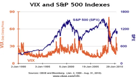
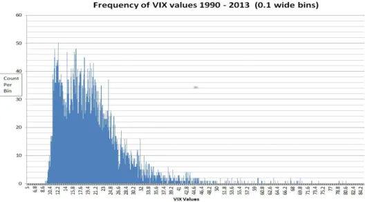
Figure 1 shows thirteen years of historical closing prices of S&P500 and VIX, in which is evident the inverse relation between the two indexes, with VIX spiking when the S&P500 index falls and then slowly mean-reverting toward lower levels. Figure 2 presents the empirical VIX closing price distribution obtained with data from 1990 to 2013. The distribution is positively skewed and leptokurtic, which is evidently in contrast with the negatively skewed distribution of returns, which is a stylized fact commonly found in market data.
The financial press has usually referred to VIX as thefear gaugeand it is currently considered as a reliable barometer of investor sentiment and market volatility. The interest expressed by several investors in trading instruments related to the market’s expectation of future volatility has lead CBOE to introduce futures and options written on VIX index, respectively in 2004 and 2006.
2.1.2
VIX Futures
The idea of a futures contract on VIX is to provide a pure play on the volatility level, independently of the direction of S&P500. These contracts are currently traded at the Chicago Futures Exchange (CFE), introduced in 2003 by the CBOE expressly to provide exchange-traded volatility derivatives.
VIX futures contracts settle on the Wednesday that is thirty days prior to the third Friday of the calendar month immediately following the month in which the applicable VIX futures contract expires. From figure 5, for example, the May 2004 (labelled as K4) contract settled on Wednesday, May 19, 2004.
The underlying is the VIX index and each contract is written on $1,000 times the VIX. The date-tsettlement valueFV IX(t, T)of a futures of tenorTis calculated
Figure 1: S&P500 and VIX index daily closing values from January 1990, to December 2003. Source: Bloomber and CBOE.
a sequence of opening prices of the SPX options considered for the VIX
calcula-tion at dateT. An extensive discussion of the settlement procedures and market
conventions of VIX futures can be found in the paper of Zhang et al. (2010). From a pricing perspective, since the VIX index is not the price of any traded asset, but just a risk-neutral volatility forecast, there is no cost-of-carry
relation-ship, arbitrage free, between VIX futures price FV IX(t, T) and the underlying
V IXt(Gr ¨unbichler and Longstaff, 1996; Zhang et al., 2010)
FV IX(t, T)6=V IXter(T−t) (2.7)
and, differently from commodity futures, there is no convenience yield either. In absence of any other market information, the model price of futures (and options) on VIX have to be computed according the risk neutral evaluation formula
FV IX(t, T) =EQ[V IXT|Ft] (2.8)
whereQdenotes the martingale pricing measure and theV IXtdynamics is
de-scribed by some model, either directly (standaloneapproach) or implied by the
S&P500 dynamics (consistentapproach), as will be discussed in the next section. The term structure of VIX Futures is the graph obtained as a map
Figure 2:VIX closing price distribution. Sample is from January 1990 to March 2013. Source: Six Figure Investing blog.
and its shape provides interesting insights on market expectations. Figure 3
pro-vides an example ofhumpedterm structure, in which acontangomarket for lower
tenors, in which investors expect future VIX (and, therefore, volatility) to rise,
is followed by abackwardationphase in which market expects volatility to calm
down somehow in the future. In figure 4, the term structure of VIX futures is plot-ted against date between February 2006 and December 2010, spanning a period before, during and after the financial crisis. The level of prices remains low and the shape of the term structure upward sloping until mid-2007, suggesting a too
low perceived value of the VIX index. The period of the crisis then raised the
overall level of the prices, but the backwarding shapes suggests that market ex-pected high volatility in the short-period, but not in the medium- to long- term. The sample period in figure 4 ends just before the beginning of the Greek debt crisis. By definition of futures contract, as datetapproaches the settlement date T, the price of the futures converges to the spot VIX value and at settlement
FV IX(T, T) =V IXT (2.10)
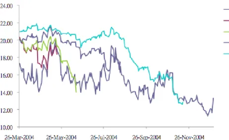
Figure 5 provides an example of this convergence with the price time series of four different contracts expiring between May and November 2004, starting from values relatively far from the corresponding VIX level and gradually converging to its level at expiration.
Figure 3:VIX futures term structure, as observed on Monday, 29 June 2009. VIX futures settle prices are in US$ and tenorT is expressed in years.
Figure 4:VIX futures term structure, as observed between February 2006 and December 2010. VIX futures settle prices are in US$. Source: Menc´ıa and Sentana (2013).
Figure 5:Pattern of VIX index value and four VIX futures settle prices: May 04, Jun 04, Aug 04 and Nov 04, settling respectively on 19 May, 16 June, 18 August and 17 November 2004. Source: The New Market for Volatility Trading(Zhang et al., 2010).
In light of the present analysis of displaced affine models, a consideration is useful for future reference: a hump in the term structure is hard to get reproduced by Heston-like affine models if calibrated consistently on both VIX futures, SPX
and VIX options, unless the instantaneous volatility processσtis extended with
the introduction of a so-called displacementφt, a positive deterministic function
which acts as a lower bound for the volatility process, that we found able to dra-matically increase the fit to the term structure of futures on VIX.
2.1.3
VIX Options
Call options on VIX with maturity T and strike K are European-style options
paying the amount(V IXT −K)+at maturity.Since they expire the same day of a
futures on VIX and subsume the same volatility reference period of 30 days start-ing from the maturity date, from equation (2.10) they can be regarded as options on a VIX futures contractFV IX(t, T)sharing expiry date with the option. This
the risk-neutral evaluation4 CV IX(K, t, T) =e−rτEQ h (FV IX(T, T)−K) + Ft i PV IX(K, t, T) =e−rτEQ h (K−FV IX(T, T)) + Ft i (2.11)
whereτ =T −tand satisfy the following put-call parity relation (Lian and Zhu,
2013, eq. 25)
CV IX(K, t, T)−PV IX(K, t, T) =e−r(T−t)(FV IX(t, T)−K) (2.12)
Moreover, no arbitrage conditions can be expressed with respect to VIX futures price (Lin and Chang, 2009)
e−r(T−t)(FV IX(t, T)−K) + ≤CV IX(K, t, T)≤e−r(T−t)FV IX(t, T) e−r(T−t)(K−FV IX(t, T)) + ≤PV IX(K, t, T)≤e−r(T−t)K (2.13)
Given the price of a call option on VIX,C∗
V IX(K, t, T), the implied volatilityσ Blk V IX(K, T)
at timetis inverted through the Black (1976) formula solving the equation (Papan-icolaou and Sircar, 2014, Sec. 2.2)
CV IXBlk (K, t, T;FV IX(t, T), r, σV IXBlk (K, T)) =C ∗ V IX(K, t, T) (2.14) where CV IXBlk (K, t, T;F, r, σ) =e− r(T−t) (FN(d1)−KN(d2)) d1= log KF +12σ2(T−t) σ√T−t d2=d1−σ √ T−t (2.15)
andN(·)denotes the CDF of the standard normal distribution function.
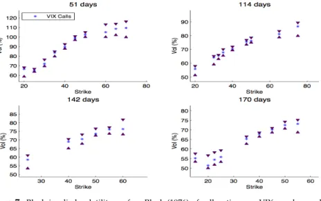
The empirical observation of S&P500 vanilla and VIX option implied volatility surfaces conveys relevant informations on the different nature of the two markets. As an example of the most evident differences between the two markets, in figure 6 we plot the Black and Scholes (1973) implied volatility surface observed on Mon-day, 29 June 2009 and in figure 7 the VIX implied surface of call options observed on the same date.
Both options datasets have been filtered using standard procedures (A¨ıt-Sahalia and Lo, 1998; Bakshi et al., 1997), as will be detailed for our empirical analysis in Chapter 4. Since VIX call options are fairly more liquid than put options, only the 4As it is usually assumed in the VIX derivative literature, the short rateris held fixed and
Figure 6: Black and Scholes (1973) implied volatility surface of europeancallsandputson S&P500, as observed on Monday, 29 June 2009. Asterisk (triangle) markers are for mid (bid/ask) price implied vols. Maturities are expressed in days and volatilities are in % points.
former have been reported in figure 7, and the price of an illiquid in-the-money (ITM) call option has been inferred from the corresponding put price via put-call parity (2.12). The SPX implied volatility surface observed in figure 6 presents typ-ical features: a negative skew more pronounced at lower maturities with OTM calls much more cheaper than corresponding puts. The VIX surface of figure 7 instead, shows rather peculiar characteristics: the implied volatility smile is up-ward sloping and the volatility level is overall higher compared to vanilla options. OTM call options on VIX are much more liquid (and are traded at higher premi-ums) than OTM puts, showing an opposite scenario with respect to options on S&P500, in which OTM puts are more expensive and heavily traded. A possible explanation for this dichotomy is the following: both puts on S&P500 and calls on VIX provide insurance from equity market downturns. On the buy-side, investors use OTM S&P500 put options to protect their portfolios against sharp decreases in stock prices and increases in volatility (Branger et al., 2014). On the sell-side, market makers that have net short positions on OTM S&P500 index puts require net long positions on OTM VIX calls to hedge their volatility risk (Chung et al., 2011). Moreover, by holding VIX derivatives investors can expose their portfolio to S&P500 volatility without need to delta hedge their option open positions with positions on the stock index. Due to this possibility, VIX options are the only asset in which open interests are highest for OTM call strikes (Rhoads, 2011).
Figure 7: Black implied volatility surface Black (1976) of call options on VIX, as observed on Monday, 29 June 2009. Asterisk (triangle) markers are for mid (bid/ask) price implied vols. Maturities are expressed in days and volatilities are in % points.
2.2
Models:
standalone
and
consistent
approach
Theoretical approaches for VIX modeling can be broadly divided in two
cate-gories: aconsistentand astandaloneapproach. The contributions considered most
relevant for this thesis will be reviewed in this section.
2.2.1
Standalone models of VIX
In the earlier standalone approach, the volatility is directly modeled, separated from the underlying stock index process. This approach only focuses on pricing derivatives written on VIX index without considering SPX options. A risk-neutral
dynamics forV IXtis usually assumed and pricing formulas as well as calibration
to VIX futures and options can be easily obtained. Within this stream of literature, theoretical contributions in modeling VIX index and pricing VIX derivatives
ap-peared well before the opening of the corresponding markets.5
5In this Section we mostly follow the review of Menc´ıa and Sentana (2013), though redefining the
TheGBMmodel of Whaley (1993)
In 1993, when VIX definition was still Black-Scholes based (i.e. VIX was what is
today known as VXO), Whaley (1993) modeledV IXt as a Geometric Brownian
Motion (GBM) under the martingale measureQ
dV IXt
V IXt
=rdt+σdWt (2.16)
The pricing formula for a VIX call optionCGBM
V IX(K, t, T)under the model (2.16)
is the Black-76 formula Black (1976), as presented in equation (2.15) and that of a futures is
FV IXGBM(t, T) =EQ[V IX
T|Ft] =V IXter(T−t) (2.17)
The GBM dynamics is both too simple to capture the dynamics of VIX, since it does not allow for mean-reversion, and to reproduce the positive implied skew of VIX options, since it yields a flat implied volatility.
The observed mean-reversion property of VIX was introduced in the subse-quent models of Gr ¨unbichler and Longstaff (1996) and Detemple and Osakwe (2000).
TheSQRmodel of Gr ¨unbichler and Longstaff (1996)
Gr ¨unbichler and Longstaff (1996) modeled the standard deviation of stock index returns as a square-root mean reverting model (Cox et al., 1985)
dV IXt=α(β−V IXt)dt+ Λ
p
V IXtdWt (2.18)
whereβis the long-term mean-reverting level,αthe rate of mean-reversion andΛ
the constant vol-of-vol parameter. Under theSQRmodel, the VIX index is
propor-tional to a non-centralχ2variable with2q+ 2degrees of freedom and parameter
of non-centrality2u, that is at any point in time the outcome of the volatility index process is distributed according to
2cV IXT |Ft ∼ χ2(2q+ 2,2u) (2.19) with c= 2α Λ2(1−e−ατ) u=cV IXte−ατ v=cV IXT q= 2αβ Λ2 −1 (2.20)
The transition pdf ofV IXtis therefore known in closed form pQ V IX(V IXT |V IXt) =ce−u−v v u q/2 Iq(2 √ uv)× I {V IXT ≥0} (2.21)
whereIq(·)is a modified Bessel function of the first kind of orderq,τ=T−tand
the indicator function is defined asI {x≥0} = 1ifx≥0and0otherwise. As a result, the price of a VIX futures is simply (Menc´ıa and Sentana, 2013, eq. 4)
FV IXSQR(t, T) =EQ[V IX
T|Ft] =β+ (V IXt−β)e−ατ (2.22)
and options on VIX can be obtained in terms of the CDFFN Cχ2(·;k, λ)of a
non-centralχ2random variable withkdegrees of freedom and non-centrality
param-eterλ(Menc´ıa and Sentana, 2013, eq. 5)
CV IXSQR(K, t, T) =V IXte−(α+r)τ1−FN Cχ2(2cK; 2q+ 6,2u)
+β 1−e−ατ 1−FN Cχ2(2cK; 2q+ 4,2u)e−rτ
−Ke−rτ
1−FN Cχ2(2cK; 2q+ 2,2u)
(2.23)
TheLOUmodel of Detemple and Osakwe (2000)
Detemple and Osakwe (2000) modeled the logV IXt as an Ornstein-Uhlenbeck
process (LOU)
dlogV IXt=α(β−logV IXt)dt+ ΛdWt (2.24)
which subsumes a log-normal conditional distribution forV IXt,
V IXT |Ft ∼ LogN µ(t, T), φ2(τ) (2.25) where µ(t, T) =β+ (logV IXt−β)e−ατ φ2(τ) =Λ 2 2α 1−e −2ατ (2.26)
and therefore, as in theSQRmodel,β andαare the long-run mean and
mean-reversion parameters, respectively. Futures on VIX are easily priced as conditional
mean of aLogN variable
FV IXLOU(t, T) =EQ[V IX T|Ft] =eµ(t,T)+ 1 2φ 2(τ) (2.27)
and the price of a call option on VIX can be expressed as a Black (1976) formula (Menc´ıa and Sentana, 2013, eq. 7), given in (2.15)
which presents a flat implied volatility across strikes, but depending on the matu-rity of the options, due to the time-dependent volatility parameterφ(τ).
BothSQRandLOUhave been extensively studied in literature: Zhang and Zhu
(2006) analyzed theSQR pricing errors on VIX futures and Dotsis et al. (2007)
studied the gains of adding jumps. The hedging effectiveness ofSQRandLOU
specifications have been tested by Psychoyios and Skiadopoulos (2006), and Wang and Daigler (2011) added options on VIX to the testing sample. Overall, as con-firmed by the extensive analysis conducted by Menc´ıa and Sentana (2013), who
considered historical VIX and VIX derivatives data6from February 2006 (opening
of VIX options market) to December 2010, theLOUdynamics yields lower
pric-ing errors compared to theSQR. Their performance tends to deteriorate during
the 2008-09 financial crisis and the underlying assumption of an exponentially
fast rate of mean reversion towards the long-run mean, poses bothSQRandLOU
models at odds with the empirical evidence, especially during bearish stock mar-kets when VIX takes long periods to revert from high levels. Moreover, both
mod-els are unable to reproduce the positive skew observed in VIX options, theLOU
yielding a flat implied volatility w.r.t. strike (for each maturity), and theSQRa negative skew.
TheSQRandLOUextensions of Menc´ıa and Sentana (2013)
The restriction of an exponential rate of mean reversion in theSQR model, is
relaxed introducing the concatenatedCSQRmodel (Bates, 2012)
dV IXt=α(βt−V IXt)dt+ Λ p V IXtdWtV IX dβt= ¯α β¯−βtdt+ ¯Λ p βtdWtβ (2.29) wherecorr(dWtV IX, dW β
t) = 0. This extension features a stochastic mean
revert-ing levelβt, which in turn reverts toward a long-rung level β¯. The stochastic
central tendencyβtdirectly affects the conditional mean ofEQ[V IXT| Ft], that is
the futures price (Menc´ıa and Sentana, 2013, eq. 10 and 11)
FV IXCSQR(t, T) = ˆβ+δ(τ)(βt−β¯) + (V IXt−βt)e−ατ δ(τ) = α α−α¯e −ατ¯ − α¯ α−α¯e −ατ (2.30)
6They use also historical data on the VIX index itself in order to estimateSQRandLOUmodels
under both under real and risk-neutral measures. Since in this thesis our focus is on derivative pricing, we do not consider explicitly real measure specifications.
but seems to be unable to reproduce the positive skew of VIX options, priced according to Amengual and Xiu Amengual and Xiu (2012)
CV IXCSQR(K, t, T) =e −rτ π Z ∞ 0 Re fV IXCSQR(z;τ)e −Kz z2 dIm(z) Re(z)< ζc(τ) := 2α Λ2 1 1−e−ατ (2.31) whereτ=T−tand fV IXCSQR(z;τ) =EQ eizV IXT Ft (2.32)
withz = Re(z) +iIm(z) ∈ C, is the conditional characteristic function of VIX
(Menc´ıa and Sentana, 2013, App. B).
Extensions of theLOUmodel are first considered separately.
• ACTOUmodel extends thelogV IXtdynamics with a time-varying central
tendency dlogV IXt=α(βt−logV IXt)dt+ ΛdWtV IX dβt= ¯α β¯−βt dt+ ¯ΛdWtβ (2.33) wherecorr(dWV IX t , dW β t ) = 0.
• In the LOUJ model, compensated λintense exponential jumps introduce
non-normality in the conditional distribution oflogV IXt
dlogV IXt=α(β−logV IXt)dt+ ΛdWtV IX+dMt
dMt=cdNt−
λ αδdt
(2.34)
whereNtis an independent Poisson process andc∼ Exp(δ).
• The constant spot volatility assumption is relaxed with theLOUSV
dlogV IXt=α(β−logV IXt)dt+ω2tdWt
dωt2=−λω2tdt+cdNt
(2.35)
whereNtis an independent Poisson process, with intensityλandc∼ Exp(δ).
The advantage of the chosen specification for the stochastic volatilityω2
t, as
compared for example with a square root dynamics, is that it allows to price futures and options onV IXtby means of Fourier inversion of its conditional
CF.
• Combining time-varying central tendency and jumps, theCTOUJmodel is obtained dlogV IXt=α(βt−logV IXt)dt+ ΛdWtV IX+dMt dβt= ¯α β¯−βt dt+ ¯ΛdWtβ dMt=cdNt− λ αδdt (2.36) wherecorr(dWV IX t , dW β
t ) = 0and jumps are as in theLOUJmodel.
• If time-varying central tendency is combined with stochastic volatility, the
CTOUSVmodel is obtained
dlogV IXt=α(βt−logV IXt)dt+ωtdWtV IX dβt= ¯α β¯−βtdt+ ¯ΛdWtβ dω2t =−λω2tdt+cdNt (2.37) wherecorr(dWV IX t , dW β
t) = 0and stochastic volatilityω2tis as in theLOUSV
model.
All the·OU·extensions of the basicLOUmodel belong to the class of the AJD
pro-cesses analyzed in Duffie et al. (2000), as shown in App. A of Menc´ıa and Sentana (2013). As a consequence, VIX derivative prices can be obtained computing the conditional CF of thelogV IXtprocess
flog·OUV IX· (z;t, T) =EQ eizlogV IXT Ft (2.38)
detailed in App. C of Menc´ıa and Sentana (2013) for all·OU·specifications. There-fore, VIX futures are easily obtained as
FV IX·OU· =flog·OUV IX· (−i;t, T)≡EQ[V IX
T| Ft] (2.39)
and VIX options can be priced applying the results of Carr and Madan (1999)
CV IX·OU· =e −αlogK π Z ∞ 0 e−iulogKψα(u)du (2.40) where ψα(u) = e−rτflog·OUV IX· (u−(1 +α)i;t, T) α2+α−u2+i(1 + 2α)u (2.41)
Their findings show that the time-varying central tendency has a deep impact in pricing futures, whereas the time-varying stochastic volatility of VIX reduces
in both markets. They find that jumps almost do not change futures prices and provide a minor improvement for VIX options. In conclusion, they give empirical support to a model of spot (log) VIX featuring time-varying central tendency and stochastic volatility, needed to capture the level and shape of VIX futures term structure, as well as the positive slope of options on VIX.
2.2.2
Consistent models of S&P500 and VIX
Although closed-form expressions for VIX derivatives prices are readily obtain-able with the standalone approach, the tractability comes at the expense of con-sistency with vanilla options. Since the same volatility process underlies both eq-uity and volatility derivatives, a reasonable model should be able to consistently price both vanilla on S&P500 and derivatives on VIX. A feature that is difficult to test if the volatility dynamics is directly modeled. Moreover, VIX index itself is computed by CBOE with a portfolio of liquid out of the money SPX vanilla, but modeling it directly does not necessarily presumes the requested replicability.
Consistent approaches retain the inherent relationship between S&P500 and VIX index. Given a risk-neutral dynamics for the S&P500 indexSt, the expression
for the VIX index in continuous time has been derived in a model-free way in terms of the risk neutral expectation of a log contract (Lin, 2007, App. A)
V IX t 100 2 =−2 ¯ τE Q log S t+¯τ F(t, t+ ¯τ) Ft (2.42)
whereτ¯ = 30/365 andF(t, t+ ¯τ) = Ste(r−q)¯τ denotes the forward price of the
underlying SPX (Duan and Yeh, 2010; Zhang et al., 2010). This expression links the SPX dynamics with that of the VIX volatility index and will be at the base of VIX derivatives pricing. Assuming a stochastic volatility affine specification·SV·,7 as it is predominant within this stream of literature, the expression (2.42) takes a simple form: it is an affine function of the stochastic volatility factorsσ2
i,tdriving the dynamics ofSt V IX·SV· t 100 2 = 1 ¯ τ n X i=1 aiσi,t2 +bi ! (2.43)
where(ai, bi)depend on the risk neutral drift of the volatility factors in the[t, t+ ¯τ]
time interval and, eventually, on the presence of jumps (both inStand/or inσ2i,t),
but not on the specification of the martingale component of the factors (Egloff et al., 2010; Leippold et al., 2007, Corollary 1).8
7SVis for Stochastic Volatility, the dots are to synthetically include the generalization of the basic
SVmodel of Heston (1993) that will be considered in the following.
8The expression in (3.15) can be derived for any·SV·model, given the dynamics ofS
Consistent models of VIX futures
Early contributions focused on the replication of the term structure of VIX futures. Zhang and Zhu (2006), assumed a risk-neutral Heston (1993) stochastic volatility
SVmodel for the SPX dynamicsSt
dSt=rStdt+StσtdWtS
dσt2=α(β−σt2)dt+ ΛσtdWtσ
(2.44)
wherecorr dWtS, dWtσ
= ρdt. Zhu and Zhang (2007), extended the (2.44)
dy-namics allowing for a time-dependent mean reverting levelβtwhich can be
cali-brated to the term structure of the forward variance
EQ[V
T| Ft] =Vte−α(T−t)+α
Z T
t
e−α(T−s)βsds (2.45)
The time-varying mean reverting levelβtis made stochastic in theSMRSVmodel
of Zhang et al. (2010), where
dβt= ¯ΛdW β t (2.46) withcorr(dWσ t, dW β
t) = 0and can be calibrated to the observed VIX futures term
structure observed in a given day. The effect of jumps in the S&P500 and volatility
dynamics has been analyzed by Lin (2007), who considered theSVCJmodel9for
xt= logSt, introduced in Duffie et al. (2000)
dxt= r−q−λµ¯−1 2σ 2 t dt+σtdWtS+cxdNt dσ2t =α(β−σt2)dt+ ΛσtdWtσ+cσdNt (2.47) wherecorr dWS t , dWtσ
= ρdt. TheSVCJmodel features correlated co-jumps,
driven by the compound Poisson processNt, with state-dependent intensityλ=
λ0+λ1σt2, exponentially distributed volatility jumpscσ ∼ Exp(µco,σ), jumps in
price conditionally normally distributedcx∼ N(µco,x+ρJcσ, δ2co,x) |cσ. The
char-acteristic function of the jump size is given by
θco(zx, zσ) =EQeicxzx+icσzσ= eiµco,xzx−12δ 2 co,xz2x 1−iµco,σ(zσ+ρJzx) (2.48)
and the compensator process isλµt¯ , withµ¯ =EQ[ecx−1] =θco(−i,0). In these models the VIX squared is as in (3.15), where
given for any model reviewed here, will be explicitly deduced for our2-SVCVJ++ model in Chapter 3 and will be generalized to a broad class of affine models for volatility derivatives in Proposition 10.
• under theSVmodel in Zhang and Zhu (2006): a(¯τ) = 1−e −¯τ α α b(¯τ) =βτ¯−a(¯τ) (2.49)
• under the time-dependent mean-reverting modelMRSVin Zhu and Zhang
(2007) a(¯τ) =1−e −τ α¯ α b(t, t+ ¯τ) = Z t+¯τ t 1−e−(t+¯τ−s)βsds (2.50)
• under the stochastic mean-reverting modelSMRSVin Zhang et al. (2010),
the VIX index depends on the instantaneous mean-reverting levelβt
a(¯τ) = 1−e −¯τ α α b(t,τ¯) =βt ¯ τ−a(¯τ) (2.51)
• under theSVCJmodel in Lin (2007), the VIX index will depend also on the
jump sizes and correlation10
a(¯τ) = 1−e −¯τ α α b(¯τ) = αβ+λµco,σ α ¯ τ−a(¯τ)+ 2λhµ¯−(µco,x+ρJµco,σ) i (2.52)
As already noted for theSQRstandalone model, outcomes of aCIRprocess (Cox
et al., 1985) are proportional to a non-central χ2 random variable. Therefore,
knowing the transition functionpQ
σ(�