by
http://ssrn.com/abstract=
1022956
Áureo de Paula and José A. Scheinkman
“The Informal Sector”
PIER Working Paper 07-033
Penn Institute for Economic Research Department of Economics University of Pennsylvania 3718 Locust Walk Philadelphia, PA 19104-6297 [email protected] http://www.econ.upenn.edu/pier
The Informal Sector
∗
´
Aureo de Paula
†University of Pennsylvania
Jos´
e A. Scheinkman
‡Princeton University and NBER
August 27, 2007
∗We thank Rita Almeida and Sandra Brand˜ao for their help with the enforcement data, Joana
Monteiro and Juliano Assun¸c˜ao for providing the ECINF dataset and for clarifying its content and methodology, and Julio Cacho and especially Paulo Natenzon, Justinas Pelenis and Glen Weyl for research assistance. We also benefited from comments by seminar participants at several institu-tions and conferences and conversainstitu-tions with William Maloney, Nicola Persico and Ken Wolpin. Scheinkman’s research was supported by the National Science Foundation through grant 0350770.
†Department of Economics, University of Pennsylvania, Philadelphia, PA 19104. E-mail:
‡Department of Economics, Princeton University, Princeton, NJ 08544. E-mail:
Abstract
This paper investigates the determinants of informal economic activity. We present two equilibrium models of informality and test their implications using a survey of 48,000+ small firms in Brazil. We define informality as tax avoidance; firms in the informal sector avoid tax payments but suffer other limitations. In the first model there is a single industry and informal firms face a higher cost of capital and a limitation on size. As a result informal firms are smaller and have a lower capital-labor ratio. When education is an imperfect proxy for ability, we show that the interaction of the manager’s education and formality has a positive correlation with firm size. These implications are supported by our empirical analysis. A novel theoretical contribution in this paper is a model that highlights the role of value added taxes in transmitting informality. It predicts that the informality of a firm is correlated to the informality of firms from which it buys or sells. The model also implies that higher tolerance for informal firms in one production stage increases tax avoidance in downstream and upstream sectors. Empirical analysis shows that, in fact, various measures of formality of suppliers and purchasers (and its enforcement) are correlated with the formality of a firm. Even more interestingly, when we look at sectors where Brazilian firms are not subject to the credit system of value added tax, but instead the value added tax is applied at some stage of production at a rate that is estimated by the State, this chain effect vanishes.
1
Introduction
In this paper we investigate the determinants of informality. It is difficult to define informal activities unambiguously, but estimates indicate that in 1990-1993 approxi-mately 10% of GDP in the United States was produced by individuals or firms that evaded taxes or engaged in illegal pursuits. It is also estimated that these activi-ties produce 25 to 35% of aggregate output in Latin America, between 13 to 70% in Asian countries, and around 15% in O.E.C.D. countries. (see Table 2 in Schneider and Enste [20]).
Informality creates a fiscal problem, but there is also growing evidence that informal firms are less efficient,1 perhaps because of their necessarily small scale,
perhaps because of their lack of access to credit or access to the infrastructure of legal protection provided by the State. In many less developed countries, creating incentives for formalization is viewed as an important step to increase aggregate productivity.
We present two related equilibrium models of the determinants of informality and test their implications using a survey of 48,000+ small firms in Brazil. In both models informality is defined as tax avoidance. Firms in the informal sector avoid paying taxes but suffer from other limitations.
The first model can be seen as a variant of Rausch [17], who relied in the modeling strategy of Lucas [14] in which managerial ability differs across agents in the economy, and assumed a limitation on the size of informal firms. We make a modification that generates additional testable implications. In addition to labor, the firms in our model use capital and informal firms face a higher cost of funds. This higher cost of capital for informal activities has been emphasized by DeSoto [5] who observed that because the right to assets held by the poor are not typically well documented “these assets cannot readily be turned into capital...[and] cannot be used as collateral for a loan. . . ”.2 This difference in interest rates induces a higher
capital-labor ratio in formal firms.3 As in Rausch [17], agents with lowest managerial ability
become workers and the ones with highest ability become formal managers, with
1Case studies reported in McKinsey [15] document that the ratio of labor productivity between
informal and formal firms is, on average, 39% in Turkey and 46% in Brazil.
2DeSoto [5], p.5-6. DeSoto [4] estimates that in June/85, informal firms in Lima (Peru) faced a
nominal interest rate of 22% per-month, while formal firms paid only 4.9% per month. We estimate a much smaller, but still significant, difference in capital costs between informal and formal firms in our sample. Straub [21] develops a model in which a dual credit system arises in equilibrium.
3Informal firms may face lower labor costs, because their workers avoid some labor taxes. This
the intermediate group running informal firms. This is because managers with more ability would naturally run larger firms and employ more capital; for this reason they choose to join the formal sector, where they do not face limits on capital deployment and face a lower cost of capital. The marginal firm trades off the cost of paying taxes versus the higher cost of capital and the scale limitations of informal firms. As a result, the marginal firm would employ in the informal sector less capital and labor than it would employ if it joined the formal sector. Thus, as in Rausch [17] or Fortin
et al. [8], a size gap develops. Managers that are slightly more efficient than the manager of the marginal informal firm employ discretely larger amounts of capital and labor.
In this class of models, entrepreneurs that operate in the informal sector are too inefficient to benefit from the lower capital costs and scale economies afforded to formal entrepreneurs. In this sense these models agree with the results from a survey of informal Mexican firms conducted by Mckenzie and Woodruff that is reported in Fajnzylberet al [7], where 75% of the respondents reported that they were too small to make it worth their while to become formal.4
Several implications of this model are supported by our empirical analysis on Brazilian data. Formalization is positively correlated with the size of firms and measures of the quality of the entrepreneurial input. Even after controlling for our measures of the quality of an entrepreneur, formalization is correlated with a firm’s capital-labor ratio or investment per worker. In addition, after controlling for the quality of the entrepreneur, formalization is correlated with higher profits.
The model predicts a correlation between manager’s ability and the size of firm. Since a manager’s ability predicts formality, formality should give no additional information concerning size, once we condition on a manager’s ability. Since ability is not observable, we study the implications of a model in which one can observe a variable, say educational achievement, that is correlated with a manager’s ability. We show that a regression of the size of the firm on this observed variable and the interaction of the observed variable and formality should produce positive coefficients. This implication is supported by our empirical results.
The main focus of our theoretical analysis is a model that highlights the role of value added taxes in transmitting informality. It exploits the idea that collecting value added taxes according to a credit scheme sets in motion a mechanism for the transmission of informality. The value added tax is a prevalent form of indirect
tion: more than 120 nations had adopted it by 2000.5 In the credit or invoice method
that is often used, the value added tax applies to each sale and each establishment receives a credit for the amount of tax paid in the previous stages of the production chain. This credit is then used by the taxpayer against future liabilities with the tax authorities. Since purchases from informal suppliers are ineligible for tax credits, an incentive exists for the propagation of informality downstream in the production chain. A similar mechanism also influences firms upstream in the chain: selling to in-formal firms increases the likelihood for a firm to be inin-formal.6 Our empirical analysis
shows that, in fact, various measures of formality of suppliers and purchasers (and its enforcement) are correlated with the formality of a firm. These findings survive when we use instrumental variables to control for possible simultaneity. Even more interestingly, when we look at sectors where Brazilian firms are not subject to the credit system of value added tax, but instead the value added tax is applied at some early stage of production at a rate that is estimated by the State, this chain effect vanishes.
Since the mid 90’s, following the lead of the Federal government, several Brazil-ian states introduced SIMPLES programs that simplified and lowered the VAT rates for small firms. The state of S˜ao Paulo, the largest and richest state in the Brazilian Federation, introduced its SIMPLES in 1998. Rio Grande do Sul, another large and relatively rich southern state, started its own program only in 2005. We use data on these two states and two rounds of the Brazilian survey of small firms to evaluate the impact of the introduction of these state programs. Our results point to a sig-nificantly positive impact of the program introduction, increasing the probability of formalization by approximately one-third.
The models in this paper ignore possible alternative reasons for informality, such as the fixed cost of complying with regulations, labor taxes or the existence of a minimum-wage. They also ignore benefits that have been highlighted in the litera-ture — such as access to participation in the legal system and other civil institutions. Considering these omitted costs and benefits should not change the qualitative im-plications of our models.
Other papers that investigate causes and determinants of informality include Loayza [13] and Friedman et al.[9] which provide evidence of an association between the size of the underground economy and higher taxes, more labor market restrictions,
5See Appendix 4 in Schenk and Oldman [19].
6To our knowledge, the only study to investigate the informal sector in conjunction with a VAT
structure is Emran and Stiglitz [6]. Their focus is on the consequences of informality for a revenue neutral tax reform involving value added and trade taxes.
and poorer institutions (bureaucracy, corruption and legal environment). Junqueira and Monteiro [11] and Fajnzylberet al.[7] are recent papers that use an earlier (1997) wave of the the survey we employ in this paper. They both explore the institution of the federal SIMPLES, which simplified and reduced rates for tax compliance for small firms in Brazil, to make inferences on the relation of taxes and informality. Although our empirical results speak to a somewhat different set of questions (for instance, the multi-stage transmission of informality captured by our second model), use data from a different year (2003 versus 1997) and refer to a different definition for formalization,7
their empirical results are broadly in line with the implications of our models. Both papers find that the enactment of SIMPLES has increased formality through a smaller tax burden and cheaper formalization costs. In particular, Fajnzylber and co-authors find that the formalization is associated with more labor and capital stocks as well as higher productivity, which agrees with the predictions of our models. They fail to obtain significant effects on formalization of participation in government assisted programmes (about which our models are silent) and access to formal credit markets.8
In sum, the combination of the models we develop and the Brazilian microdata allows us to add novel insights to this literature.
The remainder of this paper is organized as follows. In the next section we develop a model of a single industry, while in Section 3 we treat the model with two stages of production. Section 4 contains the empirical results obtained using data on informal firms in Brazil and Section 5 concludes.
7Junqueira and Monteiro [11] and Fajnzylber et al. [7] use municipal licensing as proxy for
formalization instead tax registration, the measure we use. Junqueira and Monteiro recognize that tax registration would be a more appropriate indication of formalization, but opt for licensing because the question on tax registration was only asked for those who indicated that their firm had been “legally constituted” — that is, a contract had been registered with the proper authorities. We do not view this as a problem, since according to Brazilian law only legally constituted firms are eligible for tax registration.
8In the preliminary version of Fajnzylberet al.[7] that we read, it is not clear how formal credit is
defined, but we believe it refers to bank loans. In our empirical work we use a broader interpretation of credit — 40% of those who claimed to have obtained loans (25% of the formal entrepreneurs that claimed loans) did it from non-bank sources. In addition, Fajnzylberet al.[7] focuses on firms created around the time of the introduction of the SIMPLES in 1996, just after the implementation of the Real stabilization program, when Brazilian credit markets where much less developed than in 2002. The preliminary version also contains some omissions that prevent us to make more precise comparisons (for instance, which exogenous covariates they use and whether they control for sector of activity).
2
A Model with One Production Stage
We consider a continuum of agents; each characterized by a parameter θ ≥ 0 which indicates his quality as an entrepreneur and is distributed according to a probability density functiong(·). An entrepreneur chooses between becoming a worker, operating a firm in the formal sector or in the informal sector. We assume that the production function in the two sectors is identical. If an entrepreneur employs l workers and k
units of capital, output equals y=θkαlβ, withα, β >0 and α+β <1.
A formal entrepreneur pays an ad valorem tax rate of τ and faces a capital cost of rf >0 per unit. An informal entrepreneur pays no taxes, but faces a capital
cost of ri ≥rf. All workers are paid the same wage w.
An informal entrepreneur, if detected by the authorities, loses all his profits. The probability of being detected depends monotonically on the size of the firm. Though there are several possibilities for measuring the size of the firm - output, capital stock or labor force - we choose here to use the capital stock (which we identify in the empirical work as the value of installations), because we imagine the probability of detection as a function of the “visibility” of the firm. We writep(k) for the probability of detection. While in the Appendix we discuss a more general form for the function p we will assume here that:
p(k) = 0, if k ≤k (1)
= 1, if k > k, (2) that is an informal firm cannot employ more than k units of capital, but will not suffer any penalty when k≤k.
Hence the profit for an entrepreneur of quality θ that chooses to be informal is given by
Πi(θ, ri) = max l,k≤k
{θlβkα−wl−rik}, (3)
whereas if he chooses to enter the formal sector profits will be: Πf(θ, rf) = max
l,k {θ(1−τ)l
βkα−wl−r
fk} (4)
The capital-labor ratios of formal firms or informal firms that are uncon-strained are proportional to the relative prices between labor and capital and in-dependent of the entrepreneur’s ability. Since ri ≥ rf, unconstrained informal firms
firms have a lower capital-labor ratio than unconstrained informal firms. Hence the capital-labor ratios of informal firms are lower than that of the formal firms, the difference being bigger the larger is the difference in capital costs between informal and formal firms (ri−rf). In Section 4 we provide evidence in favor of the predicted
difference in capital-labor ratios between formal and informal firms.
The usual properties of profit functions guarantee that both Πi and Πf are
convex functions of θ, w and the respective cost of capital, ri and rf. In addition the
capital and labor choices of each type of entrepreneur are monotone. Using the first order conditions and the envelope theorem one obtains :
dΠf dθ (θ) = ββ/(1−α−β)αα/(1−α−β)(1−τ)1/(1−α−β) rfα/(1−α−β)×wβ/(1−α−β) θ (α+β)/(1−α−β) , (5)
and that, for informal firms that are not constrained:
dΠi dθ (θ) = ββ/(1−α−β)αα/(1−α−β) rα/i (1−α−β)×wβ/(1−α−β)θ (α+β)/(1−α−β) , (6) If 1−τ ≥(rf ri)
α, taxes are too low with respect to the capital cost wedge and every
entrepreneur prefers to be formal. Since we are interested in the informal sector we assume from now on that 1−τ <(rf
ri)
α. In this case, every entrepreneur θ for which
the optimal choice in the informal sector is unconstrained will prefer to be informal. Let θ be the lowest value of θ for which an informal entrepreneur would choose a capital stock ¯k. For θ > θ the informal entrepreneur would keep k = ¯k and, as a consequence, in this range:
dΠi
dθ (θ) = cθ
β/(1−β), (7)
for some constantc.Comparison of this last expression with equation (5) above shows that there exists a unique θ such that Πi(θ)<Πf(θ) if and only ifθ > θ.
Each agent also has the choice of becoming a worker and receive the market wage w.Hence the occupational choice cutoff points are implicitly defined by:
Πf(θ) = Πi(θ) (8)
max{Πi(ˆθ),Πf(ˆθ)} = w (9)
and optimal choices are:
θ≤θˆ =⇒ Worker;
θ∈(ˆθ, θ] =⇒ Informal entrepreneur;
Since Πi(0) = 0 and Πf(0) = 0, ˆθ > 0, whenever w > 0. However, if θ < θˆ
then no entrepreneur would choose informality. In any case, equilibrium in the labor market requires w to satisfy:
Z max{θ(w),θˆ(w)} ˆ θ(w) li(θ;w)g(θ)dθ+ Z ∞ max{θ(w),θˆ(w)} lf(θ;w)g(θ)dθ | {z }
Demand for Labor
= Z θˆ(w) 0 g(θ)dθ | {z } Supply of Labor
where the arguments remind the reader of the dependence of the cutoffs and labor demand on the level of wages.
The existence of an equilibrium level of wages is straightforward. Also if k is small enough then θ < θ.ˆ Furthermore if θ is sufficiently large, an entrepreneur of quality θ would choose the formal sector and thus ˆθ is finite. Formal firms always exist, provided the support of g is large enough.
Another implication of this model is the existence of a discontinuity in the level of capital and labor employed at levels of productivity around θ. This discontinuity follows since an entrepreneur with ability just belowθchooses the informal sector and employs exactly k units of capital, although the marginal product of capital exceeds his cost of capital. At a level just above θ,an entrepreneur chooses the formal sector and since he is now unconstrained, he would choose a level k >> k. Furthermore, since we assumed that ri(1−τ)
1
α ≤rf and Πi(θ) = Πf(θ) we know that
Πi(θ)≤θlf(θ)βkf(θ)α(1−τ)−wlf(θ)−rikf(θ)(1−τ)1/α. Hence kf(θ)α(1−τ)> k α , and, as a consequence: θ(1−τ)βkf(θ)α w 1/(1−β) > θβk α w !1/(1−β) . (10)
The left (right) hand side of equation (10) is exactly the labor demand by a formal (informal) entrepreneur with quality θ. Hence labor demand also jumps up in the transition to formality. Thus our model predicts a “gap” in the capital and labor employed by firms near the the formalization threshold θ.
The empirical analysis of this gap is complicated because we do not observe an entrepreneur’s ability θ and the data set we use has no information on interest rates paid. In order to account for these limitations we assume that entrepreneurial ability θ = xexp() where is an unobserved determinant of entrepreneurial skill, independent of x and with zero expected value and x is some observed variable (or index of) that also influences entrepreneurship. In our empirical application we take
measures of education as proxies for x.9 In this case, one can use the expressions for
optimal input level choices to obtain the expectation of the logarithm of employment
l conditional on the logx and conditional on being in the formal or informal sector. Taking logs on the optimality conditions for labor demand and replacing θ
with xe, we get the following expression for lnl as a function of x and :
lnl= 1 1−β ln hβ w i + 1 1−β1xe≥θln(1−τ) | {z } Formalization Effect + 1 1−β(lnx+) | {z } Direct Effect + α 1−β lnk(x, ) | {z } Indirect Effect .
We highlight the fact that managerial ability influences the demand for labor in three ways. A direct effect exists since more productive entrepreneurs will demand more labor as this factor’s marginal product is higher under better management. An indirect effect occurs because a better manager will also install more capital, driv-ing up labor’s marginal productivity and hence the demand for labor. However this indirect effect will not be present for the more skilled informal managers since they will be constrained. A third effect, which we call Formalization Effect and is local to θ, occurs as entrepreneurs become formal and start paying taxes. This exerts a negative effect on the demand for labor which is nonetheless outweighed by the other two effects as pointed out previously.
If one estimates a linear regression of lnl on lnx and an interaction between lnx and formalization (θ ≥ θ) as we do in our empirical section for a sample of en-trepreneurs, the coefficient on the interaction term delivers the incremental sensitivity of lnl to lnx due to formalization. This is the sample counterpart of the best linear predictor of lnl conditional on lnx and 1xe≥θ.lnx in the population. We represent
this object as
EBLP[lnl|lnx,1xe≥θ.lnx;xe ≥θˆ] =ξ0+ξ1lnx+ξ21xe≥θ.lnx
where the conditioning eventxe ≥θˆreflects the fact that we use only entrepreneurs.
As one would expect formal entrepreneurs to employ more labor, the last term should be positive. Intuitively, in order for that to be the case, were there enough flexibility we would like to make ξ2 positive whenever lnx is positive and negative whenever
9Lazear [12] characterizes entrepreneurs as “jacks-of-all-trades who need not excel in any one skill
but are competent in many”. In this sense, managerial or entrepreneurial ability is determined in large part by balanced human capital investment. Even though better proxies may be envisioned (see for example the empirical application in that article), we take education as a reasonable determinant for the quality of an entrepreneur.
lnx is negative. This is not possible, since ξ2 is fixed. Its sign will depend on the
relatively distribution of lnx between negative and positive values. The following result can nonetheless be stated and relies on this intuition.
Proposition 1 Let x be a random variable with finite support. If supp(lnx) ⊂ R+
with at least one non-zero element then ξ2 >0.
Proof. See Appendix.
This result is used in Section 4 to document evidence in favor of our model.
3
A Model with Two Production Stages
In this section we introduce a model with two stages of production. Our goal is to illustrate the transmission of informality across sectors which results from the use of the value added tax. In Section 4 we document that this mechanism is relevant for the generation of informality in Brazil.
There are two stages of production: “upstream” and “downstream”. All in-dividuals in this model are entrepreneurs and, for simplicity, we assume that they are specialized in one of the stages. Each entrepreneur in the upstream sector is characterized by his ability θu > 0. The density of θu is gu(·). An entrepreneur of
ability θu can produce θu units of the intermediate good in the formal sector, but
only min(y, θu), where y >0, if in the informal sector.
The downstream entrepreneurs are characterized by an ability parameter θd
with density gd(·). An agent with ability θd, if in the formal sector, produces θdxα
units of the formal good using x units of the intermediate good. However if in the informal sector he faces a limit on the quantity of input that can be used and the production function becomes θdmin(x, x)α, where x >0.
We assume that gu and gd are continuous and that there exists θu < y for
which gu(θu)>0, and that gd(θd)>0 forθd >0.
The final good is tradeable and has an exogenous price q. Firms in the formal sector pay an ad-valorem tax rate of τ and we writeπ = 1−τ.The value added tax is levied by the credit method: the tax rate applies to each sale and each establishment receives a credit for the amount of tax paid in the previous stages of production. Because of the tax credit, the prices paid for informal and formal goods may be distinct and we let pf be the price of the intermediate good in the formal sector and
We write
Πuf(θu) = πpfθu (11)
Πui(θu) = pimin{θu, y} (12)
for the profit of an upstream firm with manager of quality θu if it produces in the
formal (informal) sector. Downstream firms face a slightly more complicated problem, since they must also choose which intermediate good (formal or informal) to purchase.
Write Πdf(θd) = max{max x [π(qθdx α−p fx)],max x [qπθdx α−p ix]}, (13)
for the profit of a downstream firm with a manager with ability θd that chooses to
operate in the formal sector. In an analogous manner, write Πdi(θd) = max{max x [qθdmin(x, x) α− pfx],max x [qθdmin(x, x) α− pix]}, (14)
for the profit of a downstream firm with a manager of ability θd that chooses to
operate in the informal sector.
If an informal entrepreneur of ability θd buys the input at a price p then he
demands: xi(θd, p, q) = min x, qαθd p !1/(1−α)! . (15)
In turn, a formal entrepreneur demands, if he buys from the formal sector at a unit price p: xf(θd, p, q) = qαθd p !1/(1−α) , (16)
while if he buys from the informal sector he demands xf(θd,pπ, q),since the tax credit
does not apply.
As in the model with one stage, the demand for the intermediate input, as the following proposition shows, will exhibit a large enough “discontinuity”.
Proposition 2 If Πdf(θd)>Πdi(θd) then the optimal choice of the firm with manager
of quality θd, xf(θd, p, q),where p=pf if the firm’s optimal choice is to buy the formal
good and p= pi
π if the firm’s optimal choice is to buy the informal good, satisfies
xf(θd, p, q)≥
x
π > x≥xi(θd, p, q),
Proof: Suppose first that it is optimal for the firm with manager of qualityθd to buy
the formal good. If πxf(θd, pf, q)< x, since
qθd(πxf(θd, pf, q))α−πpfxf(θd, pf, q)≥π(qθdxαf(θd, pf, q)−πpfxf(θd, pf, q)),
the firm would prefer to be in the informal sector and buy πxf(θd, pf, q) of formal
inputs. If the firm bought the informal good and πxf(θd,pπi, q)< x, since
qθd(πxf(θd, pi π, q)) α− πpixf(θd, pi π, q)≥πqθdx α f(θd, pi π, q)−πpixf(θd, pi π, q),
the firm would prefer to be in the informal sector and buy πxf(θd,pπi, q) of informal
inputs.
We now derive aggregate demand and supply of the intermediate good in the formal and informal sectors as a function of prevailing prices. Since we are interested in equilibrium prices we may restrict the range of prices to 0 < πpf ≤ pi ≤ pf. In
fact, if πpf > pi profit maximization and equations (13) and (14) imply that both
formal and informal entrepreneurs downstream would buy from informal upstream firms. However, every upstream entrepreneur will prefer to produce in the formal sector. Similarly, if pi > pf every downstream entrepreneur would prefer to buy from
formal firms. However, small θu agents would prefer to produce informally.
Further-more whenπpf ≤pi ≤pf downstream informal (formal) entrepreneurs weakly prefer
to buy from informal (formal) producers. If these inequalities are strict, preferences are also strict. In addition, the homogeneity of the system allows us to choose q = 1 (and hence we omit q as a function argument in what follows).
The following proposition shows the existence of cutoff points for each stage,
θu(pi, pf) andθd(pi, pf) such that all managers with ability below the cutoff (weakly)
prefer informality and all those with ability above the cut-off points prefer to join the formal sector.
Proposition 3 If θu < θu(pi, pf) = πppiyf ≥ y then Πui(θu) ≥ Πfu(θu), and if θu >
θu(pi, pf) = πppiy
f then Π
u
i(θu)<Πuf(θu).
(ii) There exists a θd(pi, pf) such that if θd < θd(pi, pf) then Πdi(θd)≥ Πdf(θd) and if
θd > θd(pi, pf) then Πid(θd)<Πdf(θd).
Proof: (i) is immediate from equations (11) and (12). To show that (ii) holds note thatθdenters the definition of the profit function of formal firms exactly as an output
price and hence, from the properties of profit functions with respect to output prices, we know that its derivative with respect to θd is proportional to xf(θd, p) which goes
to infinity as θd→ ∞. Furthermore, the function Πdi(θd) is convex and, since supply
functions of firms must slope up, if the choice, conditional on informality, of a firm of ability θ satisfies xi(θ) = x then the optimal choice conditional on informality,
xi(θd) =x for θd ≥ θ,and as a consequence, Πdi(θd) is linear for θd ≥θ. In addition,
whenever xi(θd)< x, the informal firm’s constraint is not binding. In this case, since
pf ≥pi Πdi =ϕ(pi)> ϕ(pf) where ϕ(p) = [αα/(1−α)−α1/(1−α)] qθd pα 1/(1−α) . Since Πdf = max{πϕ(pf), π1/(1−α)ϕ(pi)} then Πd i(θd)>Πdf(θd), provided θd>0.
Similarly to the model with one stage, the size of firms will be discontinu-ous with respect to the quality of the entrepreneur.
Proposition 4 (i) If pf > πpi the output of the smallest upstream formal firm
pfy
πpi > y.
(ii) πxf(θd(pi, pf)) ≥ x and, in particular, the output of the smallest downstream
formal firm is strictly bigger than the output of the largest informal firm.
Proof: (i) is obvious. Furthermore, the entrepreneur θd(pi, pf) must be indifferent
between being formal or informal. Since informal (formal) entrepreneurs weakly prefer to buy from informal (formal) suppliers, we must have:
θd(pi, pf)xα−pix=π θd(pi, pf)xαf(θd(pi, pf))−pfxf(θd(pi, pf)) . (17) FurthermoreF(θd) = θdxα−pix−π θd.xαf(θd)−pfxf((θd)) must satisfyF0(θd(pi, pf))≤
0. Using the envelope theorem, it follows that
xα ≤πxαf(θd(pi, pf)). (18)
Since 0< π <1 and 0< α <1, x≤πxf(θd(pi, pf)).
Because of the possibility of indifference, we have supply and demand cor-respondences as opposed to functions. We will write S(pi, pf) for the set of possible
aggregate supply vectors (si(pi, pf), sf(pi, pf)) obtained from the choices of profit
max-imizing entrepreneurs in the upstream stage. If pi 6=πpf the set S(pi, pf) contains a
single vector (si, sf) given by
si = Z piy πpf 0 min{θ, y}gu(θ)dθ (19) sf = Z ∞ piy πpf θgu(θ)dθ (20)
If πpf = pi = 0 then S(pi, pf) = {0}. Finally when πpf = pi 6= 0 a point (si, sf) ∈
S(pi, pf) if there exists aθu ≤y such that:10
si = Z θu 0 θgu(θ)dθ (21) sf = Z ∞ θu θgu(θ)dθ (22)
Since we fixed q= 1 we writeX(pi, pf) for the set of possible aggregate demand
vec-tors (xi(pi, pf), xf(pi, pf)) obtained from the choices of profit maximizing entrepreneurs
in the downstream stage.
When πpf = pi formal firms are indifferent between buying the formal or
informal input, but informal firms prefer buying from informal firms. Hence we can allocate all formal firms with managers below a certain threshold to buying in the informal sector with the complement interval assigned to purchase in the formal sector.11 In this case, a point (xi, xf)∈X(pi, pf) if there exists a γ ≥θd(pi, pf) such
that: xi = Z θd(pi,pf) 0 xi(θ, pi)gd(θ)dθ+ Z γ θd(pi,pf) xf(θ, pi π)gd(θ)dθ (23) xf = Z ∞ γ xf(θ, pf)gd(θ)dθ (24)
If πpf < pi < pf formal (informal) firms prefer to buy from formal (informal)
10In principle we could assign any subset of entrepreneurs with productivity belowyto the informal
sector, but there is always an interval containing the origin that would produce exactly the same aggregate output.
11As before, these assignments can reproduce the demands realized by any arbitrary assignment
firms. In this case, a point (xi, xf)∈X(pi, pf) if : xi = Z θd(pi,pf,1) 0 xi(θ, pi)gd(θ)dθ (25) xf = Z ∞ θd(pi,pf,1) xf(θ, pf)gd(θ)dθ (26)
If pf = pi informal firms are indifferent, but formal firms prefer buying from
formal firms. Hence we may assign informal firms arbitrarily to buying formal or in-formal inputs. In this case, a point (xi, xf)∈X(pi, pf) if there existsγ ≤θd(pi, pf,1)
such that: xi = Z γ 0 xi(θd, pi)gd(θ)dθ (27) xf = Z θd(pi,pi,1) γ xi(θd, pi)gd(θ)dθ+ Z ∞ θd(pi,pi,1) xf(θd, pi)gd(θ)dθ (28)
An equilibrium is a vector (pi, pf,1) such that ∃z ∈X(pi, pf)
T
S(pi, pf).
We will decompose the proof of the existence of an equilibrium price in two steps. First we will set pi =µpf with π ≤µ≤1. For each µwe will show that there
exists a unique pi(µ) such that if (pi, pf) = (pi(µ),piµ(µ)) then the sum of aggregate
supply of the formal and informal intermediate goods equals the sum of aggregate demands. We then show that there exits a unique µ∗ such that (pi(µ∗),pi(µ
∗)
µ∗ ,1) is an
equilibrium. We will use the following preliminary result:
Lemma 1 Ifπpf < pi < pf thenθd(pi, pf)decreases with pi and it increases with pf.
Further, if π ≤µ≤1 then, θd(pi,pµi) increases with pi.
Proof: If πpf < pi ≤pf formal firms prefer to buy the formal good. Hence
∂Πd f(θd)
∂pf
=−πxf(θd, pf) (29)
Similarly, if πpf ≤pi < pf,informal firms prefer to buy the informal good, and in an
analogous fashion
∂Πd i(θd)
∂pi
=−xi(θd, pi) (30)
This establishes the first part of the lemma, since increasing pi reduces profits for
informal firms and increasing pf reduces profits for formal firms.
1 µ ∂Πd f(θd) ∂pf − ∂Π d i(θd) ∂pi . (31)
for the marginal firm. If this is negative, the difference in profits in the formal and informal sectors for the marginal firm decreases and more firms will become informal. If πpi < pf < pi, 1 µ ∂Πdf(θd) ∂pf − ∂Π d i(θd) ∂pi =−π µxf(θd, pi µ) +xi(θd, pi). (32)
The marginal informal firm buys exactly x. Hence, from Proposition 4
−π µxf(θd, pi µ) +xi(θd, pi)≤ − x µ +x≤0
since we assume that µ≤1 and the second part of the lemma follows.
The derivative ∂Π
d f(θd)
∂pf (
∂Πdi(θd)
∂pi ) is not well defined whenpi =πpf (resp. pi =pf), but
it is easy to see that, in this case, the change in profit difference between formality and informality for the marginal firm still equals −π
µxf(θd, pi
µ) +xi(θd, pi).
We now return to the equilibrium analysis. For µ=π (pi =πpf) the sum of
the aggregate supply always equals
Z ∞
0
θgu(θ)dθ. (33)
On the other hand, the sum of aggregate demands always equals Z θd(pi,piπ,1) 0 xi(θ, pi)gd(θ)dθ+ Z ∞ θd(pi,piπ,1) xf(θ, pi π)gd(θ)dθ (34)
It is easy to check that this last expression goes to zero aspi → ∞and to∞aspi →0.
Furthermore, since demand of any type decreases with the price of the input, and, from Proposition 2 xf(θd, pi/π)> xi(θd, pi), using the Lemma above it is immediate
that aggregate demand is monotonically decreasing with pi. Hence there exists a
unique pi(π) for which the sum of supplies equal the sum of demands.
For π < µ≤1, using expressions (19) and (20) we obtain that the sum of the aggregate supplies is:
Z µyπ 0 max{θ, y}gu(θ)dθ+ Z ∞ µy π θgu(θ)dθ. (35)
On the other hand, using equations (25) and (26), the sum of the aggregate demands equals: Z θd(pi,piµ) 0 xi(θd, pi)gd(θ)dθ+ Z ∞ θd(pi,pi/µ) xf(θd, pi µ)gd(θ)dθ. (36)
Just as before, the result in the Lemma insures the monotonicity properties that yield the existence of a unique pi(µ) that equates the sum of aggregate demands with that
of aggregate supplies.
Notice that an increase inµ always decreases aggregate supply since it causes some firms in the upstream sector to switch from formal to informal. In addition, an increase in µ increases the demand by formal firms at each pi and causes some
firms to switch from informal to formal in the downstream sector. Thus, at each pi,
aggregate demand goes up. Hence pi(µ) increases with µ.
The supply of the informal sector when pi =πpf is some amount in the
inter-val [0,R0yθgu(θ)dθ]. The demand is some number in the interval
[Rθd(pi,pi/π) 0 xi(θd, pi)gd(θ)dθ, Rθd(pi,pi/π) 0 xi(θd, pi)gd(θ)dθ+ R∞ θd(pi,pi/π)xf(θd, pi/π)gd(θ)dθ].
If these intervals overlap, atpi =pi(π)/πthen (pi(π), pi(π)/π) is an equilibrium. This
will happen whenever the tolerance for informality in the upstream sector (y) is high enough.
If these intervals do not overlap, notice that the informal supply of the interme-diate good must necessarily go up withµ. On the other hand, the informal demand at (pi(µ),piµ(µ)) will go down sincepi(µ) goes up and the relative price of the formal good
goes down. Atµ= 1, the supply of the informal good isR yπ
0 max{θ, y}gu(θ)dθ whereas
the demand is any number in the interval [0,Rθd(pi,pf)
0 xi(θd, pf)gd(θ)dθ]. Hence there
always exists a unique µ∗ such that (pi(µ∗), pi(µ∗)/µ∗,1) is an equilibrium.
3.1
Comparative statics
Simulations of the model show that an increase in tolerance in the upstream sector increases the proportion of informal firms upstream and downstream. Figure 1 shows that as y increases, the proportion of upstream firms that are informal increases. As a result the price of the informal intermediate good pi decreases and some of
the downstream formal firms opt for informality. The fall in demand for the formal intermediate good causes a fall in its price pf. A symmetric picture arises when we
change the tolerance for informality in the downstream sector, x.
4
Empirical Application
In this section we explore the implications of the theoretical framework laid out in the previous section using a dataset on the informal sector in Brazil. Tax noncompliance is an important phenomenon in this country. Schneider and Enste [20] estimate that informality represents more than one-quarter of the Brazilian economy. Its value added tax system was established in the sixties and VAT represents approximately 10% of tax collection.
4.1
Data
Our principal data source is the ECINF survey (Pesquisa de Economia Informal Urbana) on informal firms realized by the Brazilian Statistics Bureau (IBGE). We use the 2003 edition of that survey, collected in October 2003, from which we obtain information on 48,701 entrepreneurs in urban regions from all states in the Brazilian federation.12 We also use the 1997 edition for the analysis present in subsection 4.9.
The focus is on units with five or less employees and the sampling strategy uses the demographic census as a frame. Before the survey, preliminary interviews screened households for the presence of at least one entrepreneur with a business employing five or less people. Households without such an entrepreneur were not included in the frame for the survey. The sampling was designed in two stages: in each state (of a total of 27) the primary sampling units (urban sectors) are stratified geographically in three strata (capital, other urban sectors in the capital metropolitan area and remaining urban sectors). In a second step, the primary sampling units were stratified according to levels of income within the geographical stratum. Urban sectors were then randomly selected with probability proportional to the number of households in the sector. From each selected urban sector a total of 16 households was then randomly selected for interviews.13. Since the focus of the survey and the definition
of informal economic unit adopted by the Brazilian statistics bureau were those firms with less than five employees and not those in irregular situation, we do believe answers were truthful even when individuals were inquired about their status with the Brazilian tax authorities. Interviewees were made aware that information collected
12When an entrepreneur owns two firms, this corresponds to two observations in our sample. When
a firm has two partners that live in the same household, this also corresponds to two observations. Initially we have 48,803 observations which are reduced to 48,701 observations after discarding data points corresponding to entrepreneurs younger than 15 yrs.-old.
for the survey was confidential and would only be utilized for statistical purposes.14
The ideal dataset for testing our second model would comprise information on the production chain associated to each firm. Although the ECINF contains certain characteristics of a firm’s clientele (whether they were predominantly large or small companies, persons or governmental institutions), this information is very limited. To complement these data we used the input-output matrix information available from the Brazilian Statistics Bureau (IBGE). We computed inter-sectoral technical input coefficients and measures of output sectoral destination using the 2003 Brazilian national accounts.15
4.2
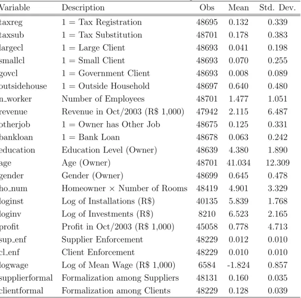
Description of Variables
We eliminated firms with owners who were less than 15 years old and the observations lacking education or gender information, what restricted our sample to around 48,000 observations.
Table 1 summarizes the main variables used in the study. The first is indicative of formalization. It is a dummy variable equal to one if the firm is registered with the Brazilian tax authorities.16 For firms in economic sectors that qualify for forward
tax substitution (see subsection 4.10 for an explanation), taxsub takes the value one. The next two variables are dummies for firms that sell their products mainly to large firms (largecl) or small firms (smallcl) (where large and small firms are those with more and less than five employees, respectively). Govcl is a dummy for a firm that sells mainly to governmental institutions. Other alternatives are persons or ignored.
Outsidehouse is a dummy that equals one when the activity is performed outside the home. The number of employees (n worker) includes the owner. Even though the survey focuses on firms with five or less employees, a few units (less than 0.1%) employ
14A disclaimer appears on top of the questionnaire stating that such information is confidential
and protected by Law 5534 14/11/68.
15Tables 1 and 2 under “Tabelas de Recursos e Usos” available under National Accounts on
http://www.ibge.gov.br for 2003. The information is at current 2003 prices (rather than the al-ternative: previous year monetary units). The construction of technical coefficients follows the European System of Integrated Economic Accounts (ESA) specifications (see ten Raa [23]).
16The tax registry is the Cadastro Nacional de Pessoas Jur´ıdicas, which replaced the previous
system, the Cadastro Geral de Contribuintes (CGC), used in the 1997 survey. This variable is the most representative of formalization for our purposes, but we have nonetheless experimented with using “legally constituted firms” and obtained virtually identical results. This is not surprising, since, as we mentioned, the latter is a prerequisite tax registration and correlation between the two measures of informality is 0.98.
more than five people due to the lag between the screening and interviewing stages of the survey and the fact that firms may have multiple partners which are also counted as employees. The variables revenue, otherjob and bankloan are self-explanatory.
Education is a categorical variable with values depicted on Table 2. Age of the owner is in years and gender equals 1 for male. The variable ho num is a measure of wealth and is zero for non-homeowners and otherwise displays the number of rooms in the house. The variables loginv and loginst measure the logarithm of investments and capital installations in October/2003 (R$ 1,000).17 Profit equals revenue minus
expenses in October/2003 (also in R$ 1,000). Logwage denotes the logarithm of the total expenditures in salaries (in R$1,000) divided by the number of employees in the firm.18 The variables (clform and supform measure formalization among customers
and suppliers of a firm (see subsection 4.7 for the construction of these variables).
[Tables 1 and 2 here]
Each firm in the sample is classified into economic activities following the CNAE (Classifica¸c˜ao Nacional de Atividades Econˆomicas) classification.19 Using
technical coefficients as well as sectoral output allocation coefficients from the Na-tional Accounts System (NAS) (using NAS sector classification) we are then able to assign to each activity in the survey a vector with those coefficients. Since the sur-vey and National Accounts use different classification schemes we had to match the activities in both systems. Typically a CNAE activity corresponds to a single NAS sector, but there are a few exceptions. Whenever such a multiple match occurred, we assigned to a CNAE sector the weighted averages (using NAS sector production value) of the coefficients in the corresponding NAS sectors. The ECINF survey also has its own aggregate sectoral characterization, displayed on Table 4.
We use these coefficients as a vector measure of sectoral allocation of output and sectoral input assignment by a firm. The last two variables on Table 1 are mea-sures of formalization enforcement for suppliers and customers20and were constructed
as follows. We used information available from the Brazilian Ministry of Labor on the number of firms visited in a given economic sector and state during 2002 to monitor
17The value of installations refers to owned installations. Rented equipment is not included. Only
7% of formal firms and 7% of informal firms reported any rented equipment
18As a reference, the annual GDP per capita in Brazil for 2003 was R$ 8,694.47 according to IBGE
(log(8.69447/12) = log(0.72454) =−0.13).
19The Brazilian Bureau of Statistics website (http://www.ibge.gov.br) provides a description of
this classification as well as various matching tables to other classification schemes.
labor regulation compliance. We normalized the number of visits in each state and sector by the number of persons employed in that state and sector provided by the Brazilian Statistics Bureau (IBGE) (through the Cadastro Central de Empresas).21
Assuming that a firm’s suppliers were in the same state, we generated an index of supplier formalization enforcement as a weighted average of these variables where the weights were the sectoral input demand coefficients. We used sectoral output alloca-tion coefficients to obtain an analogous measure of client formalizaalloca-tion enforcement.
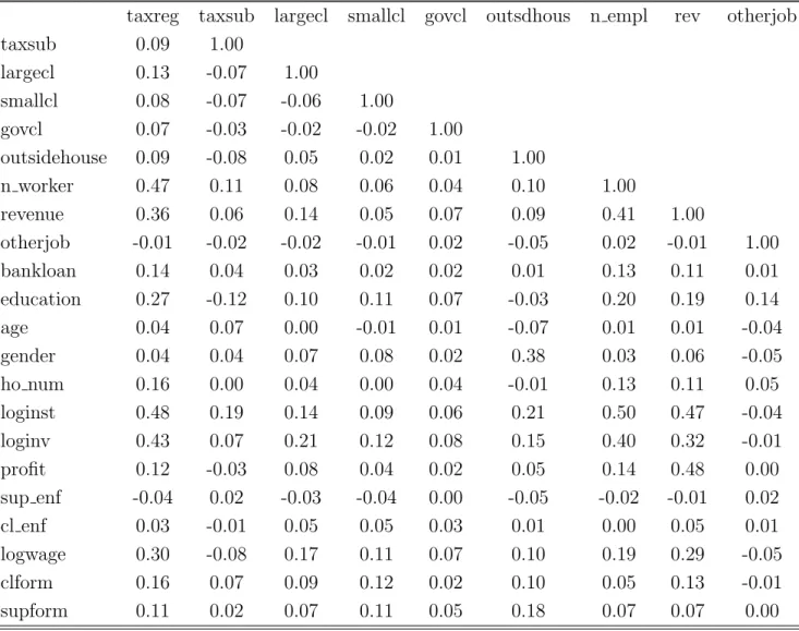
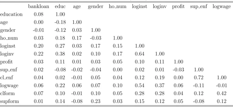
The correlation matrix for our variables is on Table 3.
[Tables 3 and 4 here]
4.3
Probability of Formalization
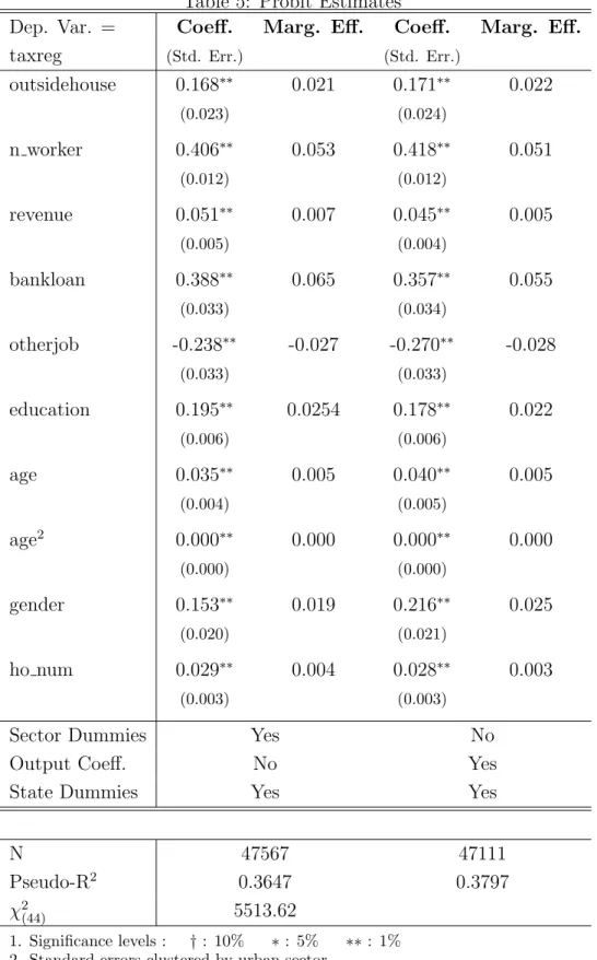
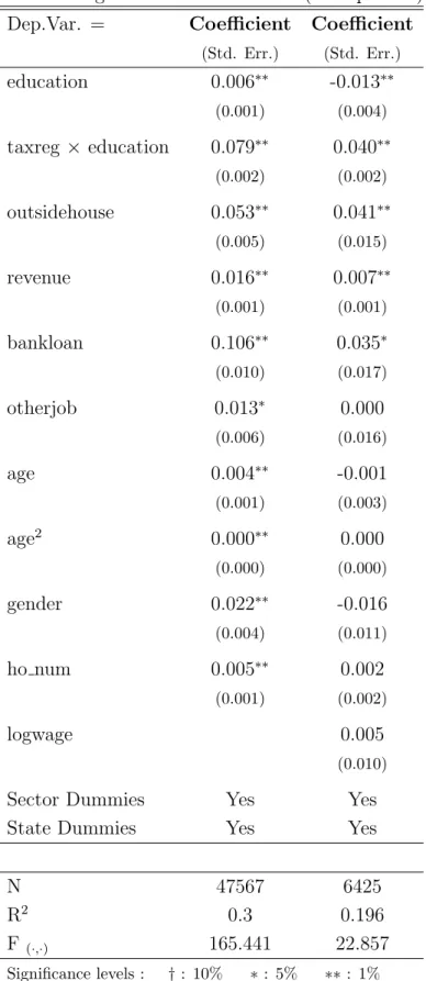
Table 5 contains probit estimates for the formalization variable taxreg using two different sets of controls. The signs obtained for each one of the regressors are as expected. The coefficient of the variable “working outside the home” is positive. In agreement with the first model, the coefficients are also positive for variables related to the size of the firm (number of employees and revenue), credit (bankloan), or the quality of the entrepreneurial input (education, age or having no additional job). Since women in Brazil are more likely to have substantial household duties, the sign on the gender variable is probably related to entrepreneurial input. The coefficients on all these variables are statistically significant.
[Table 5 here]
The two sets of estimates use different sectoral controls. In the first set we used dummies for state and sector (according to the specification on Table 4). In the second set of results we used the derived output coefficients obtained from the Brazilian National Accounts (and equivalent results are obtained if one uses the input coefficients). The National Accounts System in Brazil categorizes economic activity into forty-two sectors. The “use table” in the NAS allows one to obtain how much in a given year a sector required in terms of input from another sector in the economy. This can be used to obtain the technical coefficients for each NAS sector (see footnote 15). We were able to identify the sector (according to the NAS) for each firm in the ECINF survey using equivalence tables among the different classification schemes that are available from the Brazilian Statistics Bureau. The “make table” in the National
21Similar calculations were also performed using as normalizing variable the number of firms in
Accounts provides the quantity of output destined to each sector of the economy (plus final demand, which comprises inventory, family consumption, exports and public administration). We used this information to assemble a vector of sectoral allocation for each monetary unit of output generated for each activity in our sample (and hence each observation in our sample): (oaj)j=1,...,42. These controls, in additional to state
dummies, are used in the second set of estimates presented in the table.22
4.4
Investment, Installations per Worker and Profits
Since an entrepreneur’s true ability is not observable, it makes sense to measure the effect of formalization after controlling for characteristics of the manager and the firm. The model predicts that informal firms would choose a lower capital-labor ratio, and Table 6 depicts the effect of formalization on investments and installations per worker. The coefficient has the right sign and is statistically significant. Formalization has an economic significance of 0.31 for investments per worker and 0.52 for installations per worker regardless of the measure of formalization23. In other words, formalization is
associated with an increase in investments (installations) per worker of 0.31 (0.52) standard deviations.
[Table 6 here]
We also examined the correlation of formalization with profits. The results are summarized in the same table. Again, after controlling for characteristics of the manager and the firm, formalization has a statistically significantly positive associa-tion with profits. Formalizaassocia-tion is associated with an increase in monthly profits of approximately 700 Reais.24
4.5
Regression Regimes
In our regressions we used education as one of the measures of an entrepreneur’s qualityθ.Our model predicts a “gap” in the size distribution of firms as a function of the quality of the entrepreneur. Our observable measure for entrepreneurial quality input, education, is an integer between 1 and 8. Hence lnx ≥ 0 and Proposition 1
22For each observation we can also assemble a vector of input requirements (tc
j)j=1,...,42and these
controls result in estimates similar to the ones presented using output coefficients.
23For dummy variables, we define the economic significance as the regression coefficient divided
by the standard deviation of the dependent variable.
guarantees that the interaction coefficient is positive (provided the model is a valid description).
Table 7 exhibits OLS estimates of the number of employees on a series of controls and using education of the owner as the observable productivity enhancing feature. The coefficient of the interaction of education and formality is positive and significant. The result persists when we control for the level of wages within the firm. Since the number of employees is an integer, we also ran an ordered probit and a Poisson25 regression, but the results are very similar.
[Table 7 here]
4.6
Cost of Capital
In the first model, the marginal product of capital of formal entrepreneurs is:
α×θ(1−τ)lβkα
k =
αy(1−τ)
k .
The marginal product of capital for unconstrained informal entrepreneurs is:
α×θlβkα
k =
αy k
These quantities should then equal the cost of capital: ˜rf =δ+rf for formal
and ˜ri =δ+ri for unconstrained informal entrepreneurs, whereδ is the common rate
of depreciation. Since δ≥0 ri
rf ≥
˜
ri
˜
rf,and hence an estimate of
˜
ri
˜
rf is a lower bound for
ri
rf.With the maintained assumption thatα is the same for both formal and informal
entrepreneurs, an estimator for r˜i
˜
rf would be:
yi/ki (for unconstrained informal firm)
(1−τ)yf/kf (for formal firm)
.
In practice, neither output nor capital are perfectly measured in the survey we use. Taking revenue (net of taxes) and the value of installations as imperfect measures of output (net of taxes) and capital26, we would nonetheless obtain:
revenue installations =
y+y
k+k
25A Poisson regression models the dependence of a countable random variableY on covariatesX.
It postulates a Poisson distribution forY with expectation exp(α+β0X).
26Installations for example include facilities, tools, machines, furniture and vehicles, which may
where y and k stand for the measurement errors in output and capital, which we
assume are on average zero and uncorrelated with output and capital. Under these assumptions, the average revenue and installation values converge in large samples to the expected output and capital in the population. Conventional application of the Central Limit Theorem and the Delta Method deliver:
√ N avg revenue avg installation − E(y) E(k) =√N avg revenue avg installation − r α →dN(0,Σ)
where N is the number of observations and
Σ = σ 2 revenue E(installation)2 −2 E(revenue)σrevenue,installations E(installation)3 + E(revenue)2σinstallations2 E(installations)4
whereσ2 denote variances andσrevenue,installationsthe covariance between revenues and
installations. Σ can be estimated consistently by its sample analog which we write asΣ. We append the subscriptb iorf toN, Σ and r when referring to unconstrained informal or formal entrepreneurs respectively. The estimator relies on the assumption that the measurement error is averaged out across many randomly sampled individual and is reminiscent of the strategy used by Milton Friedman in his classical study of consumption.27
Assume now that one samples independentlyNf formal entrepreneurs andNi
unconstrained informal entrepreneurs and that Ni/Nf converges to a positive valuec
as the sample size grows. An additional application of the usual asymptotic arguments shows that the distribution of the ratio of revenue per installation for unconstrained informal entrepreneurs and for formal entrepreneurs can be approximated in large samples by
p
Nf
avg revenue
avg installationsfor unconstrained informal firms avg revenue (net of taxes)
avg installations for formal firms
− ˜ri ˜ rf ! →dN(0, V) where V = 1 (˜rf/α)2 Σi+c ˜ ri/α (˜rf/α)2 2 Σf
which again can be consistently estimated using the sample analogs for its components (for cuse actual Ni/Nf).
Among the informal firms, the unconstrained entrepreneurs are those with
27Friedman showed that cross-section regressions would underestimate the propensity to consume
since observed consumption and income are imperfect measurements of their permanent counterpart and suggested the ratio of the average consumption and average income as a better estimator for the propensity to consume.
lower skill parameter θ. Since more able entrepreneurs will employ more capital and more labor, we can use the number of workers as a sorting mechanism and focus on the group of entrepreneurs employing lower amounts of labor. Using informal employers with two or less workers leads to a point estimate of r˜i
˜
rf of 1.31 with a standard error
of 0.0178. Using informal employers with only one worker yield similar estimates. Hence we estimate that, in our data set, informal firms face a rate of interest that is at least 1.3 times the interest rate faced by formal firms.
4.7
Chain Effects on Formalization
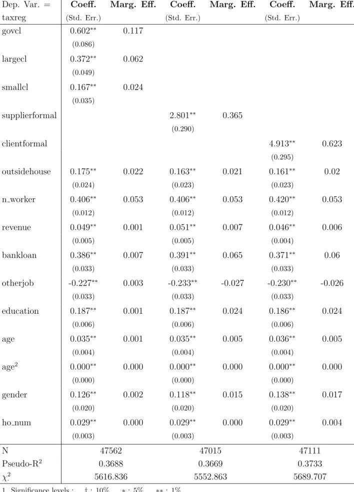
One initial approach to investigate the existence of cross-industry effects of formal-ization is to employ a characterformal-ization of a firm’s clientele as presented in the ECINF survey. Interviewees were asked to declare whether sales were principally to govern-mental institutions, large firms (more than five employees), small firms (five employees or less) or persons. Sales to governmental institutions, large firms and small firms tend to increase the probability of formalization with the largest effect being associated with governmental organizations and the lowest with small enterprises as depicted on Table 8. Since one can intuitively order these three categories according to formal-ization (with government being the most formal and large firms being more formal than small ones), we read these correlations as suggestive that there is a chain effect on formalization.
We also used a composite measure of formalization among a firm’s suppli-ers to examine the chain effect. This measure consists of a weighted average of the formalization variable (taxreg) across supplying sectors using as weights the techni-cal coefficients for input utilization from each sector. More precisely, the formality measure for the suppliers of firm i is given by
supplierf ormali = P jtcij ×formalityj P jtcij (37)
where formalityj is the percentage of firms in sector j that display tax registration28
andtcij is the required amount of input from sectorjper monetary unit of output
pro-duced by firm i (obtained from the technical coefficients for that firm’s sector). This measure of supplier’s formality only accounts for potential suppliers that are present
28Four NAS sectors were excluded since they are not sampled in the ECINF survey: agriculture,
in the survey and, in particular, ignores all suppliers that are large firms. Neverthe-less, the results of our analysis again favor the model: the coefficients attached to this variable are positive and statistically significant. The estimation results are displayed on Table 8. The marginal impact of supplier formalization on the probability of being formal is 0.365.
A similar strategy was adopted for the sales of each firm, where a sectors’ formalization is now weighted according to the output break up by sector obtainable as well from the NAS:
clientf ormali = P joaij ×formalityj P joaij (38) The results are depicted on Table 8. The coefficient on this composite measure of client formalization is positive and statistically significant, with a marginal impact of 0.623.
[Table 8 here]
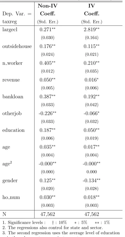
While the degree of tax compliance among a firm’s suppliers and customers seems to affect formalization, an endogeneity problem may arise since suppliers and customers of a firm respond to the degree of tax compliance of that firm. This would tend to bias the estimator upwards. Nevertheless, since the variable we use as a proxy for formalization among clients is an imperfect measure of tax compliance an extra source of endogeneity arises due to measurement error. In this case, with mismeasured categorical variables, one cannot rule out the possibility of attenuation bias in the opposite direction of the simultaneity bias (see Bound et al. [3]). To address this potential endogeneity problem we ran instrumental variable versions for the estimation results displayed in Table 8 using the average education level in the entrepreneurs urban sector as an instrument for the formalization of a firms clients. Since we use a single instrumental variable (and hence can only handle one endogenous variable), we consolidate the dummy variables indicating large firms, small firms and governmental institutions as a single variable. Table 9 display the results for the first set of estimates in Table 8 using the aggregate variable in place of largecl, smallcl
and govcl and its IV version. The coefficient on the consolidated variable, lsgecl, is positive and remains so in the IV version. In fact, the IV version displays an even larger coefficient, which we ascribe to the attenuation effects of measurement error in the non-instrumented estimation.29
[Table 9 here]
4.8
The Effect of Enforcement
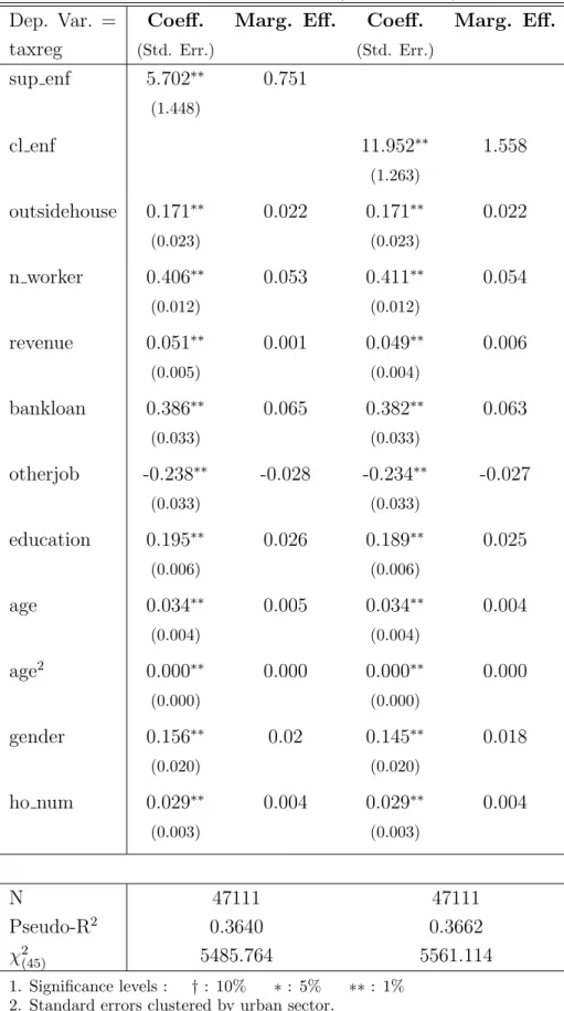
The previous results show evidence of correlation in the degree of informality across stages of production. Our second model suggests that increased tolerance towards informality in the upstream sector leads to a reduction in formalization in the down-stream sector. Similarly, higher tolerance for informality among downdown-stream firms is accompanied by higher degree of tax avoidance in the upstream sector. We use the measures of formalization enforcement in the labor market described in subsection 4.2 as an indicator for monitoring within each state-economic sector from which a firm buys (using the technical coefficients as weights) and to which a firm sells (using the output allocations as weights). Our estimates on Table 10 show that enforcement in upstream or downstream sectors has a positive and significant effect on the probability of formalization.
[Table 10 here]
4.9
SIMPLES: S˜
ao Paulo and Rio Grande do Sul
In 1996 the Brazilian federal government established the SIMPLES tax program. The program was targeted at small firms: those with roughly less than R$1,000,000 in annual revenues. It consolidated taxes and social security contributions in a single payment and aimed at simplifying the verification and remittance procedures for tax collection. Although states and municipalities were allowed to join the system for the collection of value added taxes (ICMS and ISS), very few did. More than 20 states eventually established instead their own state-level versions of the SIMPLES system for the collection of VAT and other state taxes. In 1998, the state of S˜ao Paulo established a local version of the SIMPLES program. The system exempted firms with less than R$ 120,000 annual revenues from the collection of the state VAT and offered reduced rates to larger firms with at most R$1.2 million in annual revenues. The program provided firms with a significant reduction in VAT. For example, a firm selling R$60,000 in a month with input costs at R$20,000 would pay R$7,200 in VAT before the SIMPLES. Under the new program, the VAT would amount to less than R$1,300.
We use the first round of the ECINF survey, collected in 1997, and its 2003 edition to measure the effect of this reduction in VAT on formalization in the state of
firms having only large and small firm clients and using the latter as baseline. The coefficient for the large client dummy is also positive in the non-instrumented version of this estimation and it also increases when we use the instrumental variables.
S˜ao Paulo. For comparison we use the state of Rio Grande do Sul, which established its state SIMPLES only by the end of 2005. Table 11 displays summary statistics on some key variables in 1997 for these two states. With the exception of the number of workers, the proportion of registered firms and whether the entrepreneur holds other jobs, the means for the variables are not significantly different at the 10% level.
[Table 11 here]
Table 12 displays results from a probit model where dummy variables for the state and pre- and post-introduction of the state SIMPLES are used to assess the variation in the formalization in S˜ao Paulo. We apply the controls we used in the previous formalization regressions.30 The results point to a positive impact of the pro-gram introduction with a marginal effect of 5.48 percentage points on formalization, increasing the probability of formalization by approximately one-third.
[Table 12 here]
4.10
Robustness: Tax Substitution
Brazilian tax law imposes forward tax substitution (“substitui¸c˜ao tribut´aria para frente”) in certain sectors.31 Under this tax collection system, the value added tax is charged at the initial stage in the production chain at a rate estimated by the State. This method tends to be adopted for activities with a reduced set of initial producers and many smaller units at the subsequent stages of production. Since no extra value added tax is imposed one should not expect a chain effect within these sectors.
We ran probit estimates on activities where tax substitution is imposed. These activities (and their CNAE numerical activity designation) are automobile and auto-parts manufacturing (34001, 34002, 35010, 35020, 35030, 35090), production of tires (25010), production and distribution of liquor (15050 and 53030), cigarettes (16000), commercialization of automobiles and tires (50010, 50020, 50030 and 54040), distri-bution of fuel (50050 and 53065), bars and similar establishments (55030) and oil refining (23010 and 23020).
The results concerning investment and installations, number of employees, and the entrepreneur’s education level remain qualitatively as before. In Table 13 we interact tax-substitution with our measure of formality of the clients. To facilitate
30Standard errors are not clustered by urban sector since their definition varied between 1997 and
2003.
comparisons with the results in Table 9 we again consolidate the dummy variables indicating large firms, small firms and governmental institutions as a single variable. The coefficient of the interaction term is negative and significant and the p-value of the hypothesis that the sum of the coefficients of this interaction term and the coefficient on the aggregate measure of client formalization equals zero is .0636. Hence we fail to reject at the 5% level the hypothesis that in the sectors with tax substitution there is no chain effect.
Our model predict this decrease in the interaction effect but does not make any prediction concerning the effect on the level of informality. The tax authorities in Brazil impose tax substitution hoping to increase compliance. The firms in our sample that belong to the tax substitution sectors tend to have more individuals (as opposed to firms or government) as clients and to be owned by less educated entrepreneurs, both factors associated with less formality. Nonetheless they tend to be more formal than firms in the remaining sectors. In fact the difference in the rate of formalization between firms in the tax substitution sectors and the other firms is 7.8 percentage points (with a standard error of .4), a very large effect when compared with the average level of 13.2% in our sample. This probably reflects the criterium used by the Brazilian tax authorities. Tax substitution is impose when at some level in the chain the typical producer is a large firm. If these large firms cannot afford to become informal it is likely that, through the chain effect, the smaller firms which are suppliers and buyers will tend to become formal.
[Table 13 here]
5
Conclusion
We presented two models of informality. An implications of the first model is that in-formal firms are smaller, less productive and with less capital per worker. The second model predicts that informality may be transmitted through vertical relationships when value added taxes are levied through the credit method. Using microdata from surveys conducted in Brazil, we confirmed implications of both models.
Appendix A: Proof of Proposition 1
The proof is by induction on the cardinality of supp(x), which is countable sincexis assumed discrete. The notationsuppdenotes the support of a given random variable. For a set A, #A is the cardinality of that set. Recall that we assume that ∼ G(·) is independent of x and supp() = R.
Step 1: (#supp(x) = 1) In this case, lnx is a constant and we can focus on:
EBLP[lnl|lnx,1xe≥θ.lnx;xe≥θˆ] =ϕ0+ϕ11xe≥θ
where ϕ0 =ξ0 +ξ1lnx (so that ξ0 and ξ1 are not separately identifiable) and ϕ1 = ξ2lnx. We will show that ϕ1 >0 and this in turn implies that sgn(ξ2) = sgn(lnx).
This being a best linear projection,
ϕ1 =
cov(lnl(xe),1
xe≥θ|xe≥θˆ)
var(1xe≥θ|xe ≥θˆ)
⇒sgn(ϕ1) =sgn(cov(lnl(xe),1xe≥θ|xe ≥θˆ))
where we stress the point that the equilibrium demand for labor l(xe) is a function of x and . Let solve
xe =θ⇔= lnθ−lnx
and ˆ solve
xeˆ = ˆθ⇔ˆ= ln ˆθ−lnx
The covariance can then be written as
cov(lnl,1xe≥θ|xe ≥θˆ) = Z ≥ˆ lnl(xe).1xe≥θdG(|≥ˆ) − Z ≥ˆ lnl(xe)dG(|≥ˆ). Z ≥ˆ 1xe≥θdG(|≥ˆ) = Z ≥ lnl(xe)dG(|≥ˆ)− Z ≥ˆ lnl(xe)dG(|≥ˆ).1−G() 1−G(ˆ) = G()−G(ˆ) 1−G(ˆ) Z ≥ lnl(xe)dG(|≥ˆ) − Z ˆ ≤< lnl(xe)dG(|≥ˆ).1−G() 1−G(ˆ)
Also notice that the optimal choice of labor input for an unconstrained firm is lnl(θ, r, τ) = 1 1−βlnβ+ lnθ+ 1 1−α−β ln(1−τ) + α 1−α−βlnα− α 1−α−β lnr− 1−α 1−α−βw.