The Impact of Interest Rate Risk on Bank Lending

(1)

The Impact of Interest Rate Risk

on Bank Lending

Toni Beutler

‡

, Robert Bichsel

‡

, Adrian Bruhin

§

, and Jayson Danton

§

November 5, 2015

Working Paper

Abstract

In this paper, we empirically analyze the transmission of realized interest rate risk – the gain or loss in bank economic capital due to movements in interest rates – to bank lending. We exploit a unique panel data set that contains supervisory information on the repricing maturity profiles of Swiss banks and provides us with an individual measure of interest rate risk exposure net of hedging. Our analysis yields three main results. First, our estimates indicate that a year after a permanent 1 percentage point upward shock in nominal interest rates, the average bank of 2013Q3 would ceteris paribus reduce its cumulative loan growth by approximately 170 basis points. An estimated 28% of this reduction would be the result of realized interest rate risk exposure weakening the bank’s economic capital. Second, due to the banks’ heterogeneity in interest rate risk exposure, the effect of the shock would differ across institutions and could be redistributive across regions. Finally, bank lending seems to be mainly driven by capital rather than liquidity, suggesting that a higher capitalized banking system can better shield its creditors from shocks in interest rates.

Disclaimer: The views expressed in this paper are those of the author(s) and do not necessarily represent those of the Swiss National Bank. Working papers describe research in progress. Their aim is to elicit comments and to further debate.

JEL classification:E44, E51, E52, G21

Keywords:Interest Rate Risk; Bank Lending; Monetary Policy Transmission

Corresponding Author:Adrian Bruhin, University of Lausanne, Faculty of Business and Economics (HEC Lausanne), 1015 Lausanne, Switzerland; email: adrian.bruhin@unil.ch; phone: +41 (0)21 692 34 86

(2)

Acknowledgements

We are grateful for insightful comments from Stefanie Behncke, Martin Brown, Bo Honoré, Pius Matter, Cyril Monnet, Bertrand Rime, Mark Watson, and the members of the financial stability unit of the Swiss National Bank. Any errors and/or omissions are solely our own.

(3)

1 Introduction

Banks are exposed to adverse movements in interest rates as rates on their long, fixed-term assets are on average locked-in for longer than rates on their liabilities. When the general level of interest rates rises, banks typically experience a loss in economic value as the value of assets decreases more than the value of liabilities.

An important question in that context is to what extent realized interest rate risk exposure – the gain or loss in bank economic capital due to movements in interest rates – affects bank lending. This question is particularly relevant in the current environment of prolonged low nominal interest rates in which banks have substantially increased their interest risk exposure (Turner, 2013; SNB, 2014, 2015). For instance, findings by Hanson and Stein (2015) suggest that, as nominal interest rates declined, banks have rebalanced their asset holdings towards longer maturities in order to keep the overall yield of their portfolios from decreasing too much. The theoretical literature on the transmission of monetary policy postulates that interest rate risk exposure indeed makes bank lending more sensitive to changes in nominal interest rates (Van den Heuvel, 2002, 2007). The postulated mechanism has the following intuition: If nominal interest rates rise, the resulting loss depletes a bank’s economic capital and brings it closer to regulatory or market requirements. In such a situation, the bank’s ability to restore its required capital level by issuing new equity is limited, because equity issuances are costly due to asymmetric information between existing and potential new shareholders (Myers and Majluf, 1984; Kashyap and Stein, 1995; Myers, 2001). Consequently, the bank reduces its lending in order to still comply with the capital requirements imposed by regulators or market participants.

Empirically testing how realized interest rate risk exposure affects bank lending is difficult for two reasons. First, the necessary information about interest rate sensitive balance sheet positions and the corresponding repricing maturities is often unavailable. Second, detailed information about the positions used for hedging against interest rate risk is typically not pub-licly available. Hence, constructing a measure for individual interest rate risk exposure net of hedging is often infeasible based on publicly available information.

In this paper, we address these issues by exploiting a quarterly panel data set comprising supervisory information on Swiss banks between 2001Q2 and 2013Q3. The data set provides us with an individual measure of interest rate risk exposure that directly relies on each bank’s repricing maturity profile. In a supervisory survey, each bank reports its interest rate sensitive cash flows separated by their repricing maturities, i.e. the remaining time period until the interest rate on the underlying position is reset. The repricing mismatch implied by these cash flows yields the individual measure of interest rate risk exposure. It corresponds to the adjustment in the bank’s economic value in response to a permanent 1 percentage point (pp) change in nominal interest rates over all maturities. A major advantage of this measure is that it reflects individual interest rate risk exposure net of hedging, since a bank’s reported cash flows

(4)

take eventual hedging positions into account.

We apply a dynamic panel data model that relates bank loan growth to interest rate risk exposure and various individual and macroeconomic control variables. The model, inspired by Kashyap and Stein (1995, 2000) and Gambacorta and Mistrulli (2004), enables us to estimate the most important channels through which bank loan growth responds to changes in nominal interest rates. It also allows us to estimate the sensitivity of this response to individual interest rate risk exposure.

The analysis yields three main results. First, realized interest rate risk exposure affects bank lending through its impact on economic capital. The estimated effects of a given shock in interest rates are initially small and statistically insignificant but grow over the next four quarters and eventually become highly significant. For instance, in response to a permanent 1 pp increase in nominal interest rates, the average bank in 2013Q3 would ceteris paribus reduce its predicted quarter on quarter loan growth rate by 50 basis points (bp) immediately after the shock and reduce its cumulative loan growth after one year by approximately 170 bp. An estimated 28% of the 170 bp reduction would be due to realized interest rate risk exposure lowering the bank’s economic capital. These estimated effects are also economically significant both in light of the recent increase in interest rate risk exposure and in comparison to the average quarter on quarter loan growth rate which was roughly 95 bp over the sample period or the cumulative loan growth after one year of around 380 bp.

Second, as the Swiss banks also have become more heterogeneous in their interest rate risk exposure, the effect of a permanent 1 pp increase in nominal interest rates would differ substantially across individual institutions. For example, if the average bank’s interest rate risk exposure ceteris paribus corresponded to the 1st (3rd) quartile instead of the average, it would reduce its quarter on quarter loan growth by 45 (60) bp immediately after the shock, and reduce its cumulative loan growth after one year by approximately 140 (200) bp. In historical comparison, levels of interest rate risk exposure in 2003Q1 would have seen the average bank decrease its quarter on quarter loan growth by 45 bp immediately after the shock and reduce its cumulative loan growth after one year by approximately 135 bp.

Third, bank lending seems to be mainly driven by capital rather than liquidity. In contrast to changes in economic capital due to realized interest rate risk exposure, we find no evidence that changes in excess liquidity significantly affects bank lending. This result reflects that liquidity buffers were large and most banks did not experience any strains on liquidity over the sample period.

We also used an augmented specification of the model to test whether realized gains and losses in economic capital have asymmetric effects on bank lending. The point estimates sug-gest that realized losses may have a larger effect than comparable realized gains, although the difference is not statistically significant. Thus, the above results from our baseline model may be interpreted as a lower bound for the effects of an increase in interest rates on bank lending, given current average interest rate risk exposure.

(5)

The results are relevant for policy. They indicate that taking into account the level of the banks’ exposure to interest rate risk helps to better understand how changes in interest rates affect bank loan growth. Importantly, our results suggest that individual bank loan growth has become more sensitive to changes in interest rates than it used to be prior to the recent increase in interest rate risk exposure. Although our estimates cannot be directly aggregated as they are based on individual data and do not take eventual general equilibrium effects into account, they suggest that a given upward shock in nominal interest rates would likely have a bigger impact on bank lending than in past periods where the banks’ interest rate risk exposure was lower. Moreover, the Swiss banks’ heterogeneity in interest rate risk exposure implies that even a relatively small shock could already cause sizable economic losses at the most exposed institutions that might lead them to largely curb their lending. Hence, changes in nominal interest rates could have redistributive effects; especially if the banks’ interest rate risk exposure differs across regions. Finally, the finding that capital matters more for bank loan growth than liquidity is consistent with the observations of Kishan and Opiela (2000, 2006), that a higher capitalized banking system can better shield its creditors from shocks in interest rates. The question how these results can be integrated into policy making naturally follows from our analysis but is beyond the scope of this paper.

The paper is primarily related to the existing empirical literature on bank lending. Its em-pirical strategy is similar to a seminal paper by Kashyap and Stein (2000) which analyzed the different transmission channels of monetary policy via the banking system. Bichsel and Perrez (2005) investigated how monetary policy affected bank lending in Switzerland between 1996 and 2002. However, they did not explicitly take interest rate risk exposure into account as they focused on the relative importance of capital and liquidity for bank lending. Gambacorta and Mistrulli (2004) analyzed the transmission of monetary policy in Italy between 1992 and 2001. In contrast to the former two papers, they included a supervisory measure of interest rate risk exposure. As ours, their measure of interest rate risk exposure is also based on each bank’s repricing maturity profile. However, it does not take an economic value point of view, as future cash flows are not discounted to their present value. Even though they applied an estimator that differs from ours, they also found that realized interest rate risk exposure has a strong effect on bank lending.

More recent work that is closely related to ours is by Landier et al. (2013). They estimated the impact of interest rate risk exposure of US bank holding companies on the transmission of monetary policy between 1986 and 2011. Yet, their measure of interest rate risk exposure has a different focus than ours: In contrast to our measure that is based on a supervisory survey and takes each bank’s whole maturity profile into account, their measure is based on publicly available data on each bank’s income statement and solely considers assets and liabilities that reprice within one year. Their measure is a good proxy for the maturity mismatch only under the assumption that assets and liabilities which reprice after more than a year have on average a similar duration. In contrast to our results, Landier et al. (2013)’s findings imply that banks

(6)

would on average benefit from increasing interest rates as their income gaps for maturities up to one year are on average positive.

The remainder of the paper is organized as follows. Section 2 gives an overview of the structure of the Swiss banking system and later describes the sample and variables we use in the econometric analysis. Section 3 outlines the econometric analysis. It provides background information on the main channels though which nominal interest rates can affect bank lending. Subsequently, it explains the empirical model we apply to identify how individual interest rate risk exposure affects bank lending. Lastly, it discusses how we discriminate between immediate and long-run effects, and how we deal with the specific challenges related to dynamic panel methods. Section 4 interprets the results and presents some robustness checks. Finally, section 5 concludes.

(7)

2 Data and summary statistics

This section first provides some information on the structure of the Swiss banking system. Subsequently, it discusses the sample and the variables we use in the econometric analysis.

2.1 Structure of the Swiss banking system

Table 1 summarizes the structure of the Swiss banking system. By the end of 2012, there existed 297 banks in Switzerland with total assets amounting to roughly 3.597 trillion CHF.1

Table 1: Summary Statistics on the Swiss Banking System in 2012Q4

Category Number of Domestic Client Domestic Mortgage Total Domestic Total Banks Loans Loans Loans Assets

Big Banks 2 62’395 252’147 314’542 2’183’512*

Domestically Focused Banks:

Cantonal Banks 24 47’718 289’823 337’541 482’278

Regional and Savings Banks 40 6’588 81’712 88’300 102’530

Cooperative of Raiffeisen Banks 1 7’605 135’599 143’204 164’670

Other Domestically Focused Banks 2 4’137 41’382 45’519 53’345

Other Banks 228 37’400 33’759 71’159 610’706

Banking System Total 297 165’843 834’422 1’000’265 3’597’041

Share of Big Banks 38% 30% 31% 60%

Share of Domestically Focused Banks 40% 66% 61% 22%

Notes: Figures are in millions of Swiss Francs. The category ‘total domestic loans’ includes all loans made to the real sector. The category ‘domestic client loans’ represents the difference between ‘total domestic loans’ and ‘domestic mortgage loans’ and mostly contains commercial loans. The category ‘domestically focused banks’ comprises all banks excluding the two big banks that have (i) a share of domestic loans to total assets that is greater than 50% and (ii) a volume of domestic loans of at least 280 million Swiss Francs. The term ‘domestic’ means that the borrowers of client loans are domiciled in Switzerland, and the real estates serving as collateral for mortgage loans are located in Switzerland.

Source: SNB website, annual reports for big bank assets∗and internal data.

The different types of banks fit into three main categories. The first comprises the two big banks, UBS and Credit Suisse. As internationally active universal banks, they offer a broad range of services. The second main category consists of domestically focused banks. This category contains all retail banks providing domestic loans to the real sector that amount to at least 280 million CHF and make up at least half of their total assets. In 2012Q4, there were 24 mostly state-owned cantonal banks, 40 regional and savings banks, the cooperative of Raif-feisen banks, and 2 other domestically focused banks in that category. The last main category, labeled as ‘other banks’, is made up by a heterogeneous group of mostly small banks special-ized in different business models, such as asset management, brokerage, and trade financing.

The Swiss banking system is highly concentrated. The two big banks account for just over half of its total assets. Even though roughly two thirds of their business is abroad and a large 1 _{On December 31, 2012 the nominal exchange rate was 0.91 CHF per USD.}

(8)

proportion of their balance sheet consists of financial assets, the two big banks still reached a combined market share of 31% in the market for domestic loans to the real sector in 2012Q4. However, the domestically focused banks are the most important providers of domestic loans to the real sector with a combined market share of 61% in 2012Q4 . The remaining 228 other banks play only a minor role in domestic lending to the real sector and claimed a combined market share of 8% in 2012Q4.

2.2 Sample and variables for the empirical analysis

For the empirical analysis, we build a data set that includes quarterly information on bank lending, exposure to interest rate risk, capital, liquidity and balance sheet size collected from the regular surveys conducted by the Swiss National Bank (SNB).2 _{Our sample comprises the two}

big banks and the 67 domestically focused banks and covers the period between 2001Q2 and 2013Q3. We complement the information on bank-level data with macroeconomic variables such as short- and long-term interest rates, inflation and real GDP growth.

2.2.1 Exposure to interest rate risk

Interest rate changes affect the underlying economic value of a bank’s assets, liabilities and off-balance sheet instruments, due to adjustments in the discount rates used to determine the present value of the respective future cash flows. As a consequence, the bank’s economic capital - the difference between the present value of its incoming cash flows and its outgoing cash flows - is affected by nominal interest rate movements.

Our measure of interest rate risk exposure is based on data collected from a comprehensive supervisory survey conducted by the SNB on behalf of Switzerland’s microprudential supervi-sor, the Swiss Financial Markets Supervisory Authority (FINMA). The survey provides detailed information on the repricing maturity profile of each bankiin every quartert. Banks report, on a quarterly frequency, all significant notional and interest rate cash flows arising from interest rate sensitive positions in their banking book, plus the securities and precious metal trading portfolio. Each cash flow is allocated to one of 18 time bands, according to its repricing matu-rity defined in this context as the remaining time period until the interest rate on a position is reset.3 _{Positions are differentiated, into three main categories, according to the nature of their}

interest rate repricing maturities.4 _{The first contains all positions with a defined interest rate}

repricing maturity, for example, fixed rate mortgages.5 The second category covers positions 2 _{A small number of banks only report certain variables biannually. We linearly interpolate those variables to obtain}

quarterly observations.

3 _{The 18 bands are of different lengths. There are 7 time bands for repricing below 1 year: up to 1 day, 1 day to 1}

month, 1 month to 2 months, 2 months to 3 months, 3 months to 6 months, 6 months to 9 months and 9 months to 1 year. There are 9 yearly time bands for maturities between 1 and 10 years. The longest times bands are 10 to 15 years and above 15 years.

4 _{A fourth category covers eligible capital, mostly made up of equity. We do not consider the cash flows of these}

positions as we precisely want to measure the changes in economic capital.

5 _{A 10 year fixed-rate mortgage with yearly interest payments (without pre-payment option) issued five years and}

(9)

with undefined interest rate repricing maturities such as sight claims, claims against customers and variable rate mortgage claims, on the assets side and sight liabilities and savings deposits on the liabilities side. The third category regroups remaining position without or with arbitrary interest rate repricing maturities. Cash flows of positions falling in the last two categories are reported according to the banks’ internal assumptions on interest rate repricing maturities.

For each of the 18 time bands,m, the difference between incoming and outgoing cash flows determines the net cash flow,CF(m)it. Based on these net cash flows, the bank’s interest rate

risk exposure,ρit, is given by:

ρit= 18 X m=1 CF(m)it DF(m)+1_t pp−DF(m)t , (1)

whereDF(m)tis the discount factor using the relevant risk-free interest rates for maturitymat

timet, andDF(m)+1_t ppis the hypothetical discount factor following a 1 pp increase in interest rates across all maturities.6 A positive net cash flow in time bandmleads to a reduction in the bank’s economic capital when interest rates increase. This is due to the fact that, for a given time band m, the value of assets decreases more than that of liabilities. Hence, a bank that typically extends loans with a repricing maturity exceeding that of its liabilities will experience a decrease in the value of its equity when interest rates increase. Note thatρitreflects the bank’s

interest rate risk exposure net of hedging, becauseCF(m)itcomprises all cash flows, including

those from linear hedging positions.

The measure of individual interest rate risk exposure, ρit, corresponds to the approximate

change in banki’s economic capital that would be realized per pp the risk-free nominal yield curve shifts upward. Hence, a parallel shift of the yield curve by∆it+1 pp changes bank i’s

economic capital by approximately ρit ×∆it+1 CHF. To make the realized interest rate risk

exposure comparable across banks, we express it as a fraction of eligible capital,

ρit×∆it+1

EligCit

. (2)

Figure 1 illustrates how the Swiss banks’ interest rate risk exposure evolved between 2001Q2 and 2013Q3. The orange line corresponds to the average realized interest rate risk exposure as a fraction of eligible capital, that would have occurred in response to a 1 pp upward shift in nominal interest rates. The shaded areas represent the various interpercentile ranges, along with median levels (grey line), of interest rate risk exposure.

The Swiss banks substantially increased their interest rate risk exposure over the sample period. In 2001Q2, they would on average have experienced an economic gain amounting

interest cash flow are reported in a time band corresponding to the residual maturity, ie. 4 to 5 years, and the remaining yearly interest cash flows in four distinct time bands, i.e. 9 months to 1 year, 1 to 2 years, 2 to 3 years and 3 to 4 years.

(10)

Figure 1: Interest rate risk exposure of Swiss banks −15 −10 −5 0 5 10

Exposure as a Percentage of Eligible Capital (%) 2001q3 2003q1 2004q3 2006q1 2007q3 2009q1 2010q3 2012q1 2013q3 Quarter

Average Exposure Median Percentile 25−75 Percentile 10−90 Percentile 5−95 3M Libor

Overall correlation between 3M LIBOR and Average Exposure = 0.44. Correlation before 2008Q3 = 0.29 and correlation after 2008Q3 = −0.20

to 3.75% of eligible capital if nominal interest rates increased by 1 pp, i.e. on average their liabilities had longer maturities than their assets. However, shortly after they started to increase their interest rate risk exposure. By the end of 2008, they would have incurred an average economic loss equivalent to about 4.25% of eligible capital in response to such a 1 pp increase in nominal interest rates. Since then, their interest rate risk exposure has been roughly stable on average but become more heterogeneous.

Nominal interest rates, represented by the 3 months LIBOR in red, also varied substantially between 2001Q2 and 2013Q3. The overall correlation between the 3 months LIBOR and av-erage bank interest rate risk exposure is positive. Note that the correlation before 2008Q3 is positive but negative after 2008Q3. Thus, nominal interest rates and interest rate risk exposure do not comove perfectly which helps us identify the effect of interest rate risk exposure on bank loan growth.

2.2.2 Individual bank characteristics and macroeconomic variables

Table 2 presents summary statistics of all the variables in the sample. Its upper panel con-tains individual bank characteristics, while its lower panel exhibits variables that proxy for the macroeconomic environment and are common to all banks.

The most important individual bank characteristic is the realized interest rate risk exposure as a fraction of eligible capital. We calculate it using equation (2) and proxy for the change in nominal interest rates,∆it+1, by the change in the 3 months LIBOR,∆i3t+1M. We later show

(11)

Table 2: Summary Statistics

Variable Unit Obs. Mean Std. Dev Min Max

Individual Bank Variables:

Realized Interest Rate Risk Exposure (Fraction) 3317 -0.002 0.016 -0.119 0.146 as a fraction of eligible capital

Domestic Loan Growth Rate (QoQ %) 3394 0.936 1.047 -3.755 6.028

Excess Capital (Fraction) 3412 0.525 0.348 -0.872 2.043

Normalized Excess Capital - 3412 0.000 0.348 -1.396 1.519

Excess Liquidity (Fraction) 3414 0.849 0.675 -0.425 5.751

Normalized Excess Liquidity - 3414 0.000 0.675 -1.274 4.902

Log of Total Assets (Log) 3408 14.97 1.734 12.452 21.19

Normalized Log of Total Assets - 3408 0.000 1.727 -2.354 6.218

Macroeconomic Variables:

∆Short-term interest rate (p.p.) 50 -0.068 0.312 -1.245 0.350

∆Long-term interest rate (p.p.) 50 -0.046 0.251 -0.708 0.464

Inflation Rate (YoY %) 50 0.621 0.876 -1.019 2.975

Real GDP Growth Rate (YoY %) 50 1.687 1.767 -3.138 4.089

Notes: Loan growth is a non-annualised quarter on quarter growth rate. Excess measures are defined as eligible minus required divided by required. Inflation and real GDP both represent annualised year on year quarterly rates, i.e. percentage change with corresponding quarter in the previous year. The sample period spans from 2001Q2 until 2013Q3 at a quarterly frequency. The panel data set is mildly unbalanced.

rates that also takes long term interest rates into account. Over the sample period, the realized change in economic capital due to interest rate risk exposure was close to zero on average but varied substantially over time and across banks.

The other individual bank characteristics are total domestic loans, excess capital, liquidity, and total assets. Total domestic loans are made up of domestic client and mortgage loans. They allow us to to calculate the quarter on quarter bank loan growth rate, which amounted to roughly 0.95% on average over the sample period, or 3.80% when annualized. Excess capital and liquidity correspond to the eligible minus the required amounts. To make them comparable across banks, we report them as fractions of the required amounts. On average, capitalization and liquidity exceeded the requirements by 52.5% and 84.9%, respectively. The high level of excess liquidity reflects that most banks did not experience any strains on liquidity during the sample period. We proxy for bank size by the log of total assets, which on average was 14.97.

To make excess capital, excess liquidity, and bank size easier to interpret in the econometric analysis, we apply the following normalizations. We center excess capital and excess liquidity on the entire sample mean, so that interaction terms involving these variables have an interpre-tation with respect to the average bank in the sample. Similarly, we center bank size on the sample average in each period to deal with its trending nature. We also account for outliers as well as market entries and exits in the sample. For more detailed information on the handling of outliers, the normalizations, and the treatment of market entries and exits, please refer to

(12)

appendix A.1.

Finally, to proxy for the macroeconomic environment, we add the 3 month LIBOR on CHF, the 10 year government bond yield, the inflation rate measured by the general consumer price index, and the year on year growth rate of the real GDP to the sample.

(13)

3 Empirical analysis

This section first reviews the conceptual background that provides the basis for the empirical model. Second, it describes the specification of the empirical model that allows us to identify the effects of interest rate risk exposure on bank lending. Later, it discusses how we differen-tiate between immediate and long-run effects, and how we deal with the challenges arising in dynamic panel data models.

3.1 Conceptual Background

In the empirical analysis we focus on isolating the effects of interest rate risk exposure on bank lending. To do so, we have to partial out the other main channels through which changes in nominal interest rate can affect bank lending.

A growing body of theoretical literature on the effects of monetary policy, originating from Bernanke and Blinder (1988), has analyzed market imperfections that give rise to three main channels through which changes in nominal interest rates can affect bank lending. A change in nominal interest rates can filter through: (i) the Bank Capital Channel (BCC), (ii) the Bank Lending Channel (BLC), and (iii) the Balance Sheet Channel (BSC). Each of these channels relies on distinct market imperfections, that are amplified by individual bank or borrower char-acteristics.

Our main focus lies on the BCC, which describes how a bank’s interest rate risk exposure provides the grounds for interest rate changes to shift its lending. The wider its repricing mismatch, the more exposed the bank is to interest rate risk, which increases the resulting loss in economic capital it experiences when nominal interest rates rise, and eventually reduces its lending. Van den Heuvel (2007) develops a detailed model of a bank’s asset and liability management which incorporates capital requirements and an imperfect market assumption for bank capital. In this model, the bank exhibits a maturity mismatch in its balance sheet, i.e. it relies on short-term funding to finance long-term assets, and holds a capital buffer in excess of regulatory or market requirements. If nominal interest rates rise, the bank experiences a loss in economic capital, as the interest rates on its short-term funding adjust faster than on its long-term assets. This economic loss depletes the bank’s capital buffer and brings it closer to regulatory or market capital requirements. In this situation, the bank typically does not issue new equity, as equity issuances are costly due to the asymmetric information between the banks existing shareholders and potential future shareholders (see e.g. Myers and Majluf, 1984; Kashyap and Stein, 1995; Myers, 2001). The intuition is that existing shareholders and the bank’s management know the economic value of the bank’s assets and only agree on issuing new equity if the actual share price is overvalued. However, the potential future shareholders anticipate this reasoning and are only willing to invest in newly issued equity at large discounts. Cornett and Tehranian (1994) show empirically that issuing new equity can in fact be costly. Consequently, instead of issuing new equity, the bank will cut back its loan supply in order

(14)

to still comply with the capital requirements imposed by regulators or market participants. Empirical work on Italian banks by Gambacorta and Mistrulli (2004) confirms that a wider maturity mismatch leads to a stronger reaction of bank lending to changes in nominal interest rates.

In contrast, the BLC describes how a bank’s liquidity levels determine how its loan schedule will withstand changes to the banking system’s available reserves once interest rates change. Bernanke and Blinder (1988) show with a standard IS/LM model, that the Fed’s draining of reserves and hence insured deposits, reduces the banking system’s loanable funds, ultimately decreasing the supply of bank loans. The BLC relies on the market imperfection that insured deposits carry artificially low interest rates compared to other sources of short-term funding that are not covered by deposit insurance. Thus, if a bank has to replace an outflow of insured deposits by other sources of uninsured short-term funding, its funding costs increase, and so, the bank reduces its loan supply. Kashyap and Stein (1995, 2000) provide empirical evidence for the BLC. In particular, they find that changes in monetary policy matter more for lending by small, less liquid banks.

Finally, the BSC by Bernanke and Gertler (1995) captures how raising nominal interest rates affects bank lending via altered creditworthiness of borrowers. The borrowers’ credit-worthiness deteriorates due to increased interest payments on outstanding variable rate debt. Similarly, increasing interest rates are usually associated with decreasing asset value, which erodes the borrowers’ collateral value. As a consequence, bank lending to these borrowers typ-ically decreases, as agency costs, associated with monitoring or screening rise. Jiménez et al. (2012) exploit an extensive data set on the universe of commercial loans granted by all banks in Spain to study how bank lending to firms is affected by monetary policy. One main result is that firms with weaker balance sheets and shorter creditworthy track records can rely less on external financing.

In sum, both the BCC and BLC depend on individual bank characteristics. In contrast, just like loan demand, the extent of the BSC mainly relies on individual borrower characteristics. Therefore our empirical strategy aims at isolating the BCC – our main focus of interest – along with the BLC. In contrast, it treats the BSC together with loan demand as one of the remaining components of loan growth which we cannot further disentangle explicitly, as we do not observe individual borrower characteristics.

3.2 Empirical model

We apply a dynamic panel data model of bank loan growth, inspired by Kashyap and Stein (1995, 2000) and Gambacorta and Mistrulli (2004). It allows us to estimate how interest rate

(15)

changes affect bank loan growth. The model has the following specification: ∆ lnLit=β0+α∆ lnLit−1 + 4 X s=0 β1,s ρit−1×∆i3tM EligCit−1 it−s + 4 X s=0 β2,sBit−1×∆i3t−Ms+ 4 X s=0 β3,sCit−1×∆i3t−Ms + 4 X s=0 β4,s∆i3t−Ms+ 4 X s=0 β5,s∆i10t−Ys +β6Bit−1+β7Cit−1+β8Sit−1 + 4 X s=0 β9,sCit−1×yt−s+ 4 X s=0 β10,syt−s+ 4 X s=0 β11,sπt−s + 4 X s=2 θs+µi+it, (3)

withi= 1, ..., N banks andt = 5, ..., T quarters. The dependent variable,∆ lnLit, is the first

difference of banki’s log loan volume in quartert. Hence it can be interpreted as the quarter on quarter loan growth rate. Individual bank characteristics are all lagged by one quarter to avoid simultaneity problems. Next, we explain the roles of the different regressors.

The model features one lag of the dependent variable among the regressors.7 _{This feature}

has two benefits. First, the lagged dependent variable controls for unobserved characteristics of banki’s lending in the previous periods that impact loan growth in the current period. Second, it allows for a dynamic response of the model, enabling us to differentiate between the immediate and long-run effects of an interest rate change on bank loan growth.

The parameters β1,s identify the effect of realized interest rate risk exposure as a fraction

of eligible capital. Even though the change in economic capital has no immediate P&L effect on regulatory capital, as it represents a change in the present value of future cash flows, the bank is likely to anticipate the resulting future P&L effects and adjusts its loan supply with the new information. This adjustment is in line with the BCC literature, which postulates that a bank losing part of its capital will curb its lending because its capitalization gets closer to limits imposed by regulators or market participants. Hence, we expect losses in economic capital due to realized interest rate risk exposure to have a negative effect on bank lending. This also implies that loan growth of higher exposed banks should be more sensitive to changes in nominal interest rates.

The interaction terms of normalized excess liquidity,Bit−1×∆i3t−Ms, and normalized excess

7 _{We also implemented specifications with up to four lags. In each of these specifications, we tested the joint}

significance of the additional lags. In all cases, the additional lags were never jointly significant. Furthermore, partial autocorrelation analyses suggest that the first lag is the most relevant.

(16)

capital, Cit−1 ×∆it3−Ms, with the three months LIBOR, ∆i3tM, have three interpretations. The

first interaction term controls for the notion that the loan supply of banks with larger liquid-ity buffers should be more robust to a given change in nominal interest rates, as these banks can cope longer with liquidity outflows before they have to tap into more expensive sources of uninsured short-term funding. The interpretation of the second interaction term, however, is two-fold. On the one hand, it captures that the “lemon’s premium”, i.e. the spread between the costs of insured deposits versus other sources of uninsured short-term funding, is lower for higher capitalized banks. On the other hand, an increase in interest rates generally worsens the borrowers’ financial position and may result in higher future defaults, which would need to be absorbed by the bank’s capital. If banks anticipate the higher future default rates, loan sup-ply at higher capitalized banks will react less than at lower capitalized banks since regulatory capital requirements are less binding for higher capitalized banks. The first two interpretations correspond to the BLC, while the third is in line with the BSC. In sum, we expect both of these interaction terms to have a positive effect on bank loan growth.

The specification also includes changes in the 3 months LIBOR,∆i3M

t , which proxies for

movements in short-term rates along with changes in the 10 year government bond yield,∆i10_t Y, that proxies for movements in long-term rates. The combined inclusion of these proxies for short- and long-term interest rates movements is useful given that our measure of interest rate risk exposure considers a general change in nominal interest rates over all maturities.

We further include individual bank characteristics that account for bank-specific factors that lead to heterogeneity in loan growth. First, the effect of normalized excess capital,Cit−1, on

loan growth is ambiguous. On the one hand, we expect prudent management to be associated with high capital buffers and low loan growth. On the other hand, large capital buffers could help expand loan growth by making uninsured short-term funding cheaper. Second, the effect of normalized excess liquidity, Bit−1, on loan growth is ambiguous too for similar reasons.

Large stocks of liquidity may be a result of management moving to buffer up liquidity, which, all else equal, mechanically decreases loan supply. Alternatively, large liquidity buffers may also provide a pool of loan funding. Finally, normalized size,Sit−1, most likely has a negative

coefficient, as a given absolute increase in loan volume mechanically has a smaller effect on the loan growth rate of large banks due to the bigger size of the existing loan base.

The specification additionally incorporates regressors that proxy for the economic environ-ment. We expect the interaction between normalized excess capital and the real GDP growth rate,Cit−1×yt−s, to have a negative effect on loan growth, since more solvent banks are

bet-ter positioned to withstand economic downturns, resulting in a more stable credit supply. The literature typically explains this by the fact that higher capitalized banks are more risk averse, and lend ex ante to borrowers with lower probabilities of default (see for example Kwan and Eisenbeis (1997)). The real GDP growth rate,yt, captures changes in loan demand due to the

business cycle, while the CPI inflation rate,πt, explains the part of loan growth which is simply

(17)

Finally, we allow for individual bank fixed effects, µi, which remain invariant over time

and are unique to bank i. These individual bank fixed effects absorb any potential effects of time-invariant individual characteristics of the banks that influence loan growth. In addition, we include quarter dummies,θj, to capture seasonality in bank loan growth.

3.3 Immediate and long-run effects

The dynamics that result from including the lagged dependent variable in equation (3) allow us to distinguish between immediate and long-run effects of the regressors on bank loan growth. The long-run effect of a regressor corresponds to its total cumulative impact over time under the ceteris paribus assumption that no adjustment in other variables, besides bank loan growth, takes place.

The estimate of the immediate effect of the j-th regressor directly follows from its most contemporaneous coefficient. In contrast, the estimate of its long-run effect is given by

P4

s=0βˆj,s

(1−αˆ) , (4)

i.e. by summing up all the coefficients associated with the j-th regressor and dividing by one minus the coefficient on the lagged dependent variable.8 Notice that comparing the two estimates sheds light on how much of the effect of a given shock takes place immediately upon impact.

3.4 Estimation

The estimation of dynamic panel data models may suffer from endogeneity bias due to the inclusion of lagged dependent variables among the regressors. Consider the following stylized version of our model:

yit =αyit−1+βxit+ (µi+it), |α|<1, (5)

fori= 1, ..., N andt= 2, ..., T.

A pooled Ordinary Least Squares (OLS) estimation of (5) generates an upward biased es-timate on theαcoefficient. This upward bias results from the positive correlation between the lagged dependent variable,yit−1, and the individual fixed effect,µi, in the composite error term.

Similarly, the within groups fixed effects estimator (WG) mechanically introduces a down-ward bias on theαcoefficient. This downward bias is a consequence of the negative correlation of order 1/(T −1)between the transformed lagged dependent variable, y˜it−1, and the

trans-formed error term,˜it. The literature refers to this bias as “Nickell Bias” (Nickell, 1981).

The standard way to deal with this endogeneity problem is by implementing a Generalised

8 _{Versions with further lagged dependent variables would take the following form:} P4s=0βˆj,s

(1−Pr

s=1αˆs), wherer is the

(18)

Method of Moments (GMM) approach developed by Arellano and Bond (1991), and extended by Arellano and Bover (1995) and Blundell and Bond (1998). Essentially, this GMM approach eliminates the fixed effects using a differenced equation and instruments the resulting equation with internal lagged level versions of the equation’s variables in order to alleviate the endogene-ity bias. Ultimately, GMM estimates ofαshould fall in between the OLS and WG estimates.

Note, however, that the “Nickell Bias” of the WG estimator becomes negligible when the time dimension of the panel is sufficiently large.9 _{The correlation is non-negligible for panels}

with a smallT, but becomes negligible as T increases. Excluding the additional explanatory variables, the “Nickell Bias” is given by (Nickell, 1981):

plim

N→∞

( ˆα−α)' −(1 +α)

T −1 . (6)

Therefore, a larger time dimension reduces the extent of the bias. A more general result includ-ing explanatory variables follows naturally.

Simulation studies reveal that the “Nickell Bias” becomes negligible for T > 30 (Bruno, 2005; Judson and Owen, 1999; Kiviet, 1995). In addition, any bias on the estimates of explana-tory variable coefficients depends on the relation of the explanaexplana-tory variables with the lagged dependent variable but remains slight in comparison.

Given the results of these simulation studies and the large time dimension of our panel, i.e.

T = 50, we can safely rely on the WG estimator as the “Nickell Bias” gets negligible. Us-ing the WG estimator instead of GMM estimator has two advantages. First the WG estimator is generally more efficient in practice (Arellano and Honoré, 2001; Kiviet, 1995; Alvarez and Arellano, 2003). Second, we can avoid making somewhat arbitrary choices about the instru-ment’s specific structure and the number of lags that would be necessary when implementing the GMM estimator.

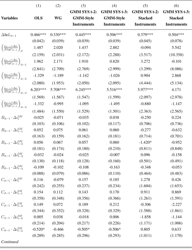
Table A2 in the appendix shows the coefficients of our model estimated using OLS, WG, and different versions of GMM. It confirms that the WG and GMM estimators yield similar results, and that the WG estimator tends to be more efficient. Consequently, all results in the following section are based on the WG estimator.

9 _{Alvarez and Arellano (2003) show that, under certain conditions, the WG estimator has the distribution}

√ N T ˆ α− α− 1 T(1 +α) d

→N(0,1−α2₎_{. Large time dimensions reduce the bias} 1

(19)

4 Results

This section first presents evidence on the importance of the different channels through which changes in nominal interest rates affect bank loan growth. Subsequently, it discusses the impact of realized rate risk exposure on bank loan growth. In addition, it explores whether the effects of gains and losses due to realized interest rate risk exposure are different in absolute terms. Finally, it summarizes the results of four robustness checks.

4.1 Effect of interest rate changes on bank loan growth

Table 3 exhibits the estimated effects of the different channels through which changes in nomi-nal interest rates may affect bank loan growth. For a given change in nominomi-nal interest rates,∆i, the first column shows the immediate effects, while the second column contains the long-run effects under the assumption that no adjustment takes place in other variables apart from bank loan growth. The long-run estimates can be interpreted as approximate cumulative effects over the next year, since the weights of future periods decline at a geometric rate and any period after four quarters in the future has an almost negligible weight.

Table 3: Immediate vs. Long-run Effects

Variables Immediate Long-Run

Realized Interest Rate Risk Exposureρit−1×∆i3tM

EligCit−1

2.02 11.51***

as a fraction of eligible capital (2.03) (3.32)

Norm. Excess Liquidity×∆i3M _–0.07 _–0.08

(0.11) (0.15)

Norm. Excess Capital×∆i3M _–0.08 _–0.48

(0.25) (0.90)

∆Short-term interest rate(∆i3M₎ _–0.38** _–1.09**

(0.17) (0.45)

∆Long-term interest rate(∆i10Y₎ _–0.07 _–0.23

(0.08) (0.31)

Notes: Dependent variable is the first difference of log quarterly loan volume, i.e. ap-proximately the quarter on quarter loan growth rate. Estimates using the Within Groups transformation in Table A2. All standard errors, in parentheses, are cluster robust at a bank-merger level. Immediate effect standard errors are simply regression estimates. Long-run effect standard errors are calculated using the delta-method. The long-run ef-fects work under the assumption that no adjustment takes place in other variables apart from bank loan growth. In addition, the long-run estimates can be interpreted as approxi-mate cumulative effects over the next year. ***p <0.01, **p <0.05, *p <0.1

The estimates in the first row indicate that changes in nominal interest rates affect bank loan growth to a large extent through the effect of realized interest rate risk exposure on eco-nomic capital. The corresponding long-run effect is statistically highly significant, while the immediate effect is insignificant. This result is consistent with the intuition that anticipated

(20)

losses in economic capital alter bank lending in future periods. To get a first interpretation of the magnitude of the effect, consider how a 1 pp upward shift in nominal interest rates af-fects two hypothetical banks, A and B, that only differ in interest rate risk exposure. Bank

A would experience an economic loss equivalent to 5% of its eligible capital if interest rates rise by 1 pp over all maturities, i.e. ρAt/EligCAt−1 = −5%. BankB, on the other hand, is

relatively more exposed and the economic loss would amount to 6% of its eligible capital, i.e.

ρBt/EligCBt−1 =−6%.10 The estimated coefficients indicate, that bankB’s quarter on quarter

loan growth would be lower by −0.05−(−0.06)×1pp×2.02 = 2.02bp thanA’s imme-diately after the shock, and its cumulative loan growth after one year would be approximately −0.05−(−0.06)×1pp×11.51 = 11.51bp lower. Hence, we find evidence for a strong BCC in Switzerland that is driven by realized interest rate risk exposure.

In contrast, changes in nominal interest rates have no significant effect on bank loan growth via the levels of excess liquidity or excess capital. Hence we find neither evidence for a BLC, acting through excess liquidity and the bank’s “lemon’s premium”, nor for a BSC, acting through higher anticipated default rates. An explanation for the absence of a BLC and BSC in our data may be that, over the sample period from 2001Q2 to 2013Q3, the vast majority of Swiss banks did not experience any strains on liquidity and Switzerland’s real economy was stable, so that defaults among borrowers were relatively rare. Moreover, many cantonal banks enjoy implicit or explicit state guarantees that may render the “lemon’s premium” they have to pay for uninsured short-term funding small and irresponsive to their level of excess capital.

Finally, the direct impact of both the short- and long-term interest rates on bank loan growth capture the remaining supply and demand effects, which we cannot further disentangle. The co-efficients on the short-term interest rates are large in absolute value and significant, while those on the long-term interest rates remain smaller in absolute value and statistically insignificant.

4.2 Ceteris paribus effect of interest rate risk exposure

We now explore in more detail the extent to which interest rate risk exposure affects the sen-sitivity of bank loan growth to movements in nominal interest rates. In particular, we analyze the ceteris paribus effect of interest rate risk exposure for a permanent 1 pp increase in nominal interest rates over all maturities on the average bank in the sample.

The solid black line in Figure 2 represents the predicted change in the average bank’s cu-mulative loan growth in response to such a permanent 1 pp increase in nominal interest rates happening at timet.11 _{To predict the immediate effect, i.e. in}_t_{, we take the model’s most}

con-temporaneous coefficients and evaluate equation (3)’s derivative with respect to∆it= ∆i3tM = ∆i10_t Y = 1pp at the average bank’s characteristics in timet.12 To predict how the effect evolves

10_{Note that the same result could also be obtained by holding interest rate risk exposure constant,}_ρ

At=ρBt, but assuming different levels of eligible capital between A and B. However, different levels of eligible capital would also affect other characteristics of the mode in equation (3).

11_Time_t_{refers to the last available period in our sample, i.e. 2013Q3.} 12_{Calculation details can be found in appendix A.3.}

(21)

Figure 2: Cumulative effect of a permanent 1 percentage point upward shock in nominal interest rates on bank loan growth

−200

−150

−100

−50

Cumulative effect on loan growth (bp)

t t+1 t+2 t+3 t+4

Quarters after shock

Exposure equal to 1. quartile Average Bank Exposure equal to 3. quartile Calculation details can be found in appendix A.3.

over the subsequent quarters, i.e. overt+s, s = 1. . .4, we have to take the dynamics of the model into account as described in appendix A.3.

The dashed lines in Figure 2 illustrate the ceteris paribus effect of interest rate risk exposure. They correspond to the predicted response of the average bank’s cumulative loan growth to the permanent 1 pp increase in nominal interest rates, assuming that its interest rate risk exposure equals the 1st and 3rd quartile, respectively, while keeping all other characteristics constant. Consequently, the dashed lines represent the average bank’s predicted reaction to the interest rate increase, if it had an interest rate risk exposure corresponding to 1st and 3rd quartile, respectively.13

Comparing the solid and dashed lines in Figure 2 reveals that interest rate risk exposure has a substantial impact on the sensitivity of bank loan growth. Immediately after the 1 pp shock in nominal interest rates, the predicted decline in quarterly loan growth amounts to 50 bp for the average bank in the sample. However, if, ceteris paribus, this bank had an interest risk exposure equal to the 1st or 3rd quartile, respectively, the predicted decline would instead amount to 45 bp and 60 bp. In the long-run, the impact of interest rate risk exposure gets even bigger, as the widening spread between the dashed lines illustrates. A year after the shock, i.e. in t+ 4, the cumulative predicted decline in the average bank’s loan growth is 170 bp.14

13_{Appendix A.7 contains individual figures including the 95% prediction intervals.}

14_{Remember that the total impact over time works under the ceteris paribus assumption that no adjustment in other}

(22)

A decomposition of this predicted decline illustrates that roughly 28% of the decline is due to realized interest rate risk. In comparison, for an interest rate risk exposure equal to the 1st or 3rd quartile respectively, the total predicted decline would, ceteris paribus, amount to 140 bp or 200 bp. In these cases, the contribution of interest rate risk exposure to the predicted declines amounts to 11% and 40% respectively.

The substantial impact and vast heterogeneity of interest risk exposure indicate that the decline in loan growth following an interest rate shock would not only be large in magnitude but also vary greatly across banks. In particular, if nominal interest rates were to increase suddenly, we expect the highly exposed banks in the sample to cut back their lending substantially more than the average bank.

4.3 Differences in the effects of gains and losses

The results presented in Table 3 rely on the assumption that gains and losses in economic capital due to realized interest rate risk exposure have a symmetric effect on bank loan growth. How-ever, this assumption may not be met in reality, especially since short-term nominal interest rates have approached the zero lower bound, even venturing into negative rates. To test for po-tential asymmetries in the effects of gains and losses, we estimated an augmented specification of our model. We included a dummy variable that allows the realized interest rate risk expo-sure as a fraction of eligible capital to have a different effect on bank loan growth depending on whether the exposure lead to a gain or a loss. (See appendix A.4 for further details).

Table 4: Asymmetry of Interest Rate Exposure

EligCit−1

: as a fraction of eligible capital

Gain 0.79 9.57

(2.29) (5.75)

Loss 4.13 15.60**

(4.37) (6.40)

Two-sided test for equal coefficients (p-value):

H0: Gains=Losses

0.50 0.54

Ha: Gains6=Losses

Notes: Dependent variable is the first difference of log quarterly loan volume, i.e. ap-proximately the quarter on quarter loan growth rate. Estimates using the Within Groups transformation. All standard errors, in parentheses, are cluster robust at a bank-merger level. Immediate effect standard errors are simply regression estimates. Long-run effect standard errors are calculated using the delta-method. The long-run effects work under the assumption that no adjustment takes place in other variables apart from bank loan growth. In addition, the long-run estimates can be interpreted as approximate cumulative effects over the next year. ***p <0.01, **p <0.05, *p <0.1

(23)

Table 4 summarizes the results. The point estimates suggest that realized losses may have a larger impact on bank loan growth than realized gains. In comparison to the coefficients of the baseline model, reported in Table 3, the estimated long-run effect of realized losses is roughly 30% higher. These results suggest that upward shocks in nominal interest rates that typically lead to economic losses given the observed exposures likely have a larger effect on bank lending than comparable downward shocks that typically lead to economic gains. However, since the difference between the estimated effects of realized gains and losses in economic capital are far from being statistically significant, we stick with the baseline model and interpret its estimates as a lower bound for the effects of realized interest rate risk on bank lending.

4.4 Robustness Checks

This subsection presents four main robustness checks. First, we use an alternative measure for the change in nominal interest rates to calculate the realized change in economic capital due to interest rate risk exposure. Second, we check whether the results remain robust when we exclude the two big banks from the sample. Third, we assess whether the unbalanced nature of the panel influences the results. Finally, in the fourth robustness check, we exclude the first seven quarters during which the average bank’s interest rate risk exposure was positive.

4.4.1 Alternative proxy for the change in nominal interest rates

In the baseline specification, we use the change in the 3 months LIBOR to determine the real-ized change in economic capital due to interest rate risk exposure. Hence, we implicitly assume that changes in short-term rates convey the necessary information for calculating the realized interest rate risk exposure. We now relax this assumption and alternatively proxy for the change in nominal interest rates by the average change between the 3 months LIBOR and 10 year gov-ernment bond yield, ∆iavg_t . To check whether our results remain robust, we reestimate the empirical model using the resulting alternative definition of realized interest rate risk exposure as a fraction of eligible capital,

ρit−1×∆iavgt

EligCit−1

(24)

Table 5: Robustness – Alternative Interest Rate Measure

Realized Interest Rate Risk Exposureρit−1×∆iavgt

EligCit−1

0.80 14.02***

(0.11) (0.15)

(0.25) (0.90)

∆Short-term interest rate(∆i3M₎ _–0.39** _–1.05**

(0.15) (0.44)

(0.09) (0.32)

Table 5 shows that the results remain robust. Even though the point estimates suggest a slight shift of focus from the immediate effect towards the long-run effect, they are not signifi-cantly different from the estimates of the baseline model reported in Table 3.

We repeat the ceteris paribus analysis of the effect of interest rate risk exposure found in section 4.2, but use the estimated coefficients from Table 5. The results indicate that immedi-ately after a 1 pp shock in nominal interest rates, the predicted decline in quarter on quarter loan growth amounts to 46 bp for the average bank in the sample. A year after the shock, i.e. in

t+ 4, the cumulative predicted decline in the average bank’s loan growth would be 155 bp. In this case, the decomposition of this predicted decline illustrates that roughly 38% of the decline is due to realized interest rate risk.

4.4.2 Excluding the two big banks from the sample

The baseline estimation uses the sample which includes the two big banks along with the do-mestically focused banks. On the one hand, including the big banks provides a more complete picture of the Swiss banking system. But on the other hand, it is problematic due to the big banks’ international business models and specific reporting requirements. In particular, the fol-lowing two issues compromise the quality of our measure of interest rate risk exposure for the two big banks.

First, about two thirds of the two big bank’s business is located abroad. This affects both the numerator and the denominator of the measure of interest rate risk exposure ρit. In the

(25)

the big banks’ economic capital, as it neglects that most of the big banks’ cash flows are in foreign currencies. Similarly, in the denominator, our measure likely overestimates the amount of eligible capital the big banks attribute to domestic lending.

Second, since the measureρit relies on the repricing mismatch between assets and

liabili-ties, it is an adequate measure for interest rate risk arising from the banking book. However, in contrast to the domestically focused banks, the two big banks both have a substantial trading book for which the repricing mismatch is a less adequate measure of interest rate risk.

Table 6: Robustness – Without Big Banks

EligCit−1

2.65 11.96***

(0.11) (0.14)

(0.27) (0.92)

∆Short-term interest rate(∆i3M₎ _–0.36** _–1.34***

(0.16) (0.45)

(0.09) (0.31)

In light of these issues, we excluded the big banks from the sample and re-estimated our baseline model. As Table 6 reveals, the estimates we obtain are virtually identical to the ones shown in Table 3. Consequently, the two big banks have only a negligible impact on our results.

4.4.3 Assessing the influence of the unbalanced panel data

Another concern could be that the unbalanced nature of the panel data set influences the results. Although the sample period from 2001Q2 to 2013Q3 coversT = 50quarters, we only observe 62 banks over the whole period.15 Another 8 banks either left – mainly due to mergers and acquisitions – or newly entered the sample between 2001Q2 and 2013Q3. To check whether the unbalanced nature of the panel data set has an influence on the results, we re-estimated our model including only banks which we observe for at least 10, 15, and 20 periods. As shown in 15_{24 Cantonal, 33 regional and savings banks, Raiffeisen Group banks, Bank Coop, Bank Migros and the two big}

(26)

Table A5 in the appendix, the results remain robust.

4.4.4 Excluding quarters with positive interest rate risk exposure

In the first seven quarters of the sample, i.e. from 2001Q2 to 2002Q4, the banks were on average positively exposed to upward interest rate shocks, meaning that they would have ex-perienced an economic gain if nominal interest rates increased. This period of positive interest rate risk exposure is unusual and may reflect that, due to flat yield curves, typical maturity transformation was no longer as beneficial. As a result, asset duration was reduced culminating in positive exposure to upward interest rate shocks. To check whether our results remain robust, we excluded these seven quarters from the sample and re-estimated our baseline model on the restricted sample period from 2003Q1 to 2013Q3.

We find that the coefficients on the impact of realized interest rate risk exposure on bank lending remain robust, although they are estimated less precisely. The other coefficients are ro-bust too, with the exception that the estimated direct effect of short-term interest rates becomes significantly larger in absolute terms. Consequently, the estimated total effect of a permanent change in nominal interest rates on bank lending is larger in the restricted sample, but the es-timated effect of realized interest rate risk exposure remains virtually unchanged. Detailed results can be found in Table A.6 in the appendix.

(27)

5 Conclusion

Our results are policy relevant in various ways. First of all, they indicate that the level of banks’ exposure to interest rate risk needs to be taken into account when trying to understand how changes in interest rates affect bank loan growth. Our results suggest that individual bank loan growth has likely become more sensitive to changes in interest rates than it used to be prior to the recent increase in interest rate risk exposure. Even though our estimates cannot be directly aggregated as they are based on individual data and do not take eventual general equilibrium effects into account, they still indicate that a given upward shock in nominal interest rates would probably have a greater effect on bank lending in Switzerland today than experience prior to the recent increase in interest rate risk exposure suggests. Furthermore, as the Swiss banks have become more heterogeneous in interest rate risk exposure, even a relatively small shock could already cause substantial losses in economic capital at the most exposed institutions, and lead them to significantly cut back their lending. In parallel, if interest rate risk is heterogeneous across regions, an interest rate shock may have redistributive effects. Finally, the finding that bank lending is mainly driven by capital rather than liquidity suggests that larger capital buffers would make bank lending more resilient against shocks in nominal interest rates, while larger liquidity buffers would only have a relatively small or even no effect. Similar conclusions are drawn in recent work published in BIS (2015).

However, a few limitations regarding our measure of interest rate risk are in order here. It is exclusively based on the loss in economic capital due to banks’ repricing mismatches. Thus it ignores that, in the current environment of negative short-term interest rates, an upward shock in nominal interest rates would benefit the banks in two ways: They would have to pay less negative interest rates on their sight deposit accounts at the SNB and, at the same time, their liability margin would be restored.16 These two effects could at least partly offset the economic loss arising from repricing mismatches. On the other hand, our measure may underestimate the banks’ true exposure to interest rate risk, as their assumptions regarding positions with undefined repricing maturities may be too optimistic; especially if the shock is substantial, and interest rates on deposits need to be adjusted faster than expected.

Finally, there is scope for future research. An important open question is how changes in the maturity of bank lending affects the transmission of monetary policy. On the one hand, our results suggest that increased interest rate risk exposure renders bank lending to the real sector more sensitive to changes in nominal interest rates. But on the other hand, increased repricing maturity of loans at the origin of increased interest rate risk exposure also temporar-ily shields existing borrowers from changes in interest rates. Furthermore, as loan-level data 16_{The liability margin is the difference between the alternative funding costs for the corresponding maturity on the}

capital market and the interest paid on the actual liability. It recently became negative for most banks. After the introduction of negative interests on sight deposits at the SNB, some capital and money market interest rates became negative too, while the interest rates on customer sight and savings deposits remained close to zero but positive (SNB, 2015).

(28)

becomes more readily available, accounting for borrower characteristics that fall under the bal-ance sheet channel of monetary policy transmission should become possible. In summary, our results should prove helpful for better understanding the transmission of monetary policy via the banking system. As such our results constitute only a first step towards the integration of banking sector characteristics into policy making, an important question that is beyond the scope of this paper.

(29)

References

Financial Stability Report 2014. Swiss National Bank, 2014.

Interest rate risk in the banking book. Consultative Document. Bank for International Settle-ments, June 2015.

Financial Stability Report 2015. Swiss National Bank, 2015.

Javier Alvarez and Manuel Arellano. The time series and cross-section asymptotics of dynamic panel data estimators. Econometrica, 71(4):1121–1159, 2003.

Manuel Arellano and Stephen Bond. Some tests of specification for panel data: Monte carlo evidence and an application to employment equations. The review of economic studies, 58 (2):277–297, 1991.

Manuel Arellano and Olympia Bover. Another look at the instrumental variable estimation of error-components models. Journal of econometrics, 68(1):29–51, 1995.

Manuel Arellano and Bo Honoré. Panel data models: some recent developments. Handbook of econometrics, 5:3229–3296, 2001.

Ben S Bernanke and Alan S Blinder. Credit, money, and aggregate demand. The American Economic Review, pages 435–439, 1988.

Ben S Bernanke and Mark Gertler. Inside the black box: The credit channel of monetary policy.

The Journal of Economic Perspectives, 9(4):27–48, 1995.

Robert Bichsel and Josef Perrez. In quest of the bank lending channel: evidence for switzerland using individual bank data. Swiss Journal of Economics and Statistics, 141(2):165–190, 2005.

Richard Blundell and Stephen Bond. Initial conditions and moment restrictions in dynamic panel data models. Journal of econometrics, 87(1):115–143, 1998.

Stephen R Bond. Dynamic panel data models: a guide to micro data methods and practice.

Portuguese economic journal, 1(2):141–162, 2002.

Giovanni SF Bruno. Approximating the bias of the lsdv estimator for dynamic unbalanced panel data models. Economics Letters, 87(3):361–366, 2005.

Marcia Millon Cornett and Hassan Tehranian. An examination of voluntary versus involuntary security issuances by commercial banks: The impact of capital regulations on common stock returns. Journal of Financial Economics, 35(1):99–122, 1994.