Keyword Optimization in Search-Based Advertising Markets

(1)

Tel Aviv University

Raymond and Beverly Sackler Faculty of Exact Sciences The Blavatnik School of Computer Science

Keyword Optimization in Search-Based Advertising

Markets

Thesis submitted in partial fulfillment of the requirements for the M.Sc. degree of Tel-Aviv University

by

Yuval Netzer

The research work for this thesis has been carried out at Tel-Aviv University under the supervision of

(2)

Acknowledgements

I am heartily thankful to my supervisor, Prof. Yishay Mansour, whose encouragement, guidance and endless patience allowed me to complete this thesis.

I would also like to thank my loved wife and kids Iris, Itai and Avigail, all who have supported me in this research, each in their own way :)

Last, I offer my regards and blessings to all of those who supported me in any respect during the completion of this project.

(3)

Search-based advertising is a multi-billion industry which is part of the growing electronic commerce market. In this work, we study the search-based advertising market from the advertiser’s point of view. There are three natural participants in the search-based ad-vertising: the advertisers, promoting their products to consumers based on their search queries, the users, which are searching for content, and the search providers, who match the advertisers and users by placing ads in search result pages. It is customary today for the advertisers to pay only for ad clicks. This guides both the advertisers’ and the search providers’ strategy. The advertisers’ strategy, which is the focus of this work, requires them to select keywords, bids and a budget constraint imposed on their advertising spending. We abstract an optimization problem in which the advertisers set a daily budget and select a set of keywords on which they bid. We assume that the cost and benefit of keywords is fixed and known, sidestepping this important strategic issue and focusing on the keyword optimization problem. The advertisers’ goal is to optimize the utility subject to its budget constraint. Clearly the advertisers would like to buy the most profitable keywords, subject to the budget constraint. The problem is that there is uncertainty regarding the type and number of queries in a day, and the advertisers have to fix a single policy for the online day. If too few keywords are selected, the advertisers remain with unused budget. If too many keywords are selected, at the time keywords associated with ’good’ ads appear, the daily budget may have already been exhausted.

We study the advertisers’ keyword optimization problem in three different settings: in an offline problem setting in which all problem parameters are known beforehand, in a stochastic model in which the advertiser knows only some of the parameters of the stochastic model, and in an adversarial model which makes no statistical assumptions about the generation of the query sequences. For each of these models we provide lower and upper bounds to the performance of learning algorithms while using the notion of regret minimization [1].

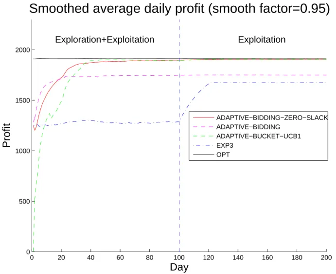
We support our theoretical results with extensive simulations in a simulated environ-ment while comparing our algorithm’s performance against the performance of algorithms suggested in [3].

(5)

Chapter 1

Introduction

1.1

Search-Based Advertising

In the last decade, search-based advertising has become a multi-billion industry and a market of major interest for many companies. Search-based advertising is a method of placing online advertisements on Web pages that show results from search engine queries. These advertisements are targeted to match key search terms (keywords) queried on search engines. Consumers often use the search engine to identify and compare purchasing options immediately before making purchasing decisions. The opportunity to present consumers with advertisements tailored to their immediate buying interests encourages consumers to click on search ads instead of unpaid search results, which are often less relevant. This highly focused targeting ability has contributed to the attractiveness of search advertising for advertisers.

Search based advertising usually takes the following form: when an Internet user enters a search query into a search engine, he gets back a page with results, containing both the links most relevant to the query and additional sponsored links which are advertisements. These sponsored links are distinguishable from the ”organic” search results presented, and different searches yield different sponsored links. When a user clicks on these sponsored links, he is sent to the advertisers Web page. A company whose ad is displayed pays the search engine only when the consumer clicks on the ad. For each such click, the advertiser pays the search engine a payment determined by the auction mechanism, which is used by the search engines to sell the online advertising.

The three main players taking place in the search-based advertising market are the advertisers, the search engines and the consumers (search engine users):

1. The advertisers are companies or individuals interested in promoting their products to consumers based on their search queries. In most search-based advertising services, a company sets a daily budget, selects a set of keywords, determines a bid price for each keyword, and designates one or more ads associated with each selected keyword. The companies try to maximize their utility of this budget and measure metrics such as cost per click (CPC) and conversion rates (the percentage of clicks that result in a commissionable activity, i.e., sale or lead).

2. The search engines - in order to determine which ads to present given a user query, the search engines conduct auctions to sell ads according to bids received for keywords matching the query and the relative relevance of the user query to the ads in the inventory. Since the search engine is paid only for clicks, it is in its interest to present advertisement on which the user is likely to click. The number of ads that the search

(6)

engine can present to a user is limited, and different positions on the search results page yield different results, e.g., an ad shown at the top of a page is more likely to be clicked than an ad shown at the side. The mechanism most widely used by search engines are based on the generalized second-price (GSP) auction [2]. In a GSP auction the bidder pays the minimal bid that is required to get the position he was assigned.

3. Consumers - when a consumer searches using a search engine, their queries are matched against advertiser’s selected keywords. The search engines then display the ads associated with the highest quality scores for those keywords on the search result page. The quality scores combine the bids and signals such as the keywords’ expected clickthrough rates.

The advertisers, who wish to promote their goods and services via search-based adver-tising, need to decide between millions of available keywords and a highly uncertain click-through rate associated with the ads matched to them. Identifying the most profitable set of keywords, given the daily budget constraint, is a challenging task. This challenging optimization problem is the subject of this work.

In the rest of this chapter we describe related work and our main thesis results.

1.2

Keyword Optimization in Search-Based

Advertis-ing

Keyword optimization for search based advertising has been the focus of some theoretical and applicative work.

Rusmevichientong and Williamson ([3]) have formulated a model for keyword selection in search based advertising. In their model, the advertiser has a fixed daily budget and each keyword has fixed known cost and profit. However, the keyword click-through probabilities are unknown. The number of queries appearing in each of the days, as well as the distribu-tion of keywords, are generated probabilistically with known parameters. They justify their assumptions about keyword costs and distribution by identifying multiple public available data sources that may be used to estimate these parameters.

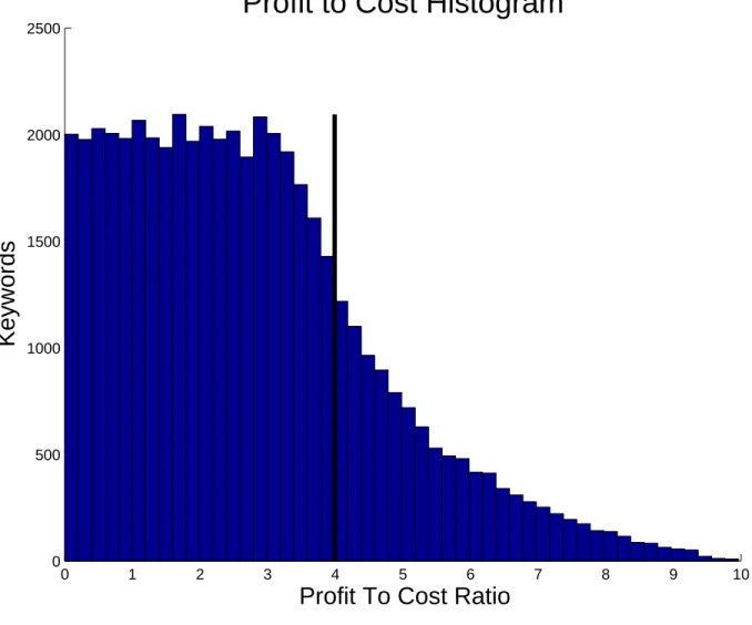
The main result of [3] is to develop an algorithm that adaptively identifies a set of keywords to bid on, based on historical performance. The algorithm uses a prefix of a sorted list of keywords, which are sorted by descending order of profit-to-cost ratios, and uses an approximation algorithm for the stochastic knapsack [4]. They prove that by considering only subsets of keywords that are prefix, they achieve near optimal profits while reducing the size of the decision space from 2N _to _N_{, where} _N _{is the number of keywords}

in the problem. The policy adaptively selects prefix keywords in order to maximize the total expected profit. There is a tradeoff between selecting too few profitable keywords, and not exhausting the entire daily budget, versus selecting too many keywords, and thus losing opportunities to receive clicks from profitable words that may arrive after the daily budget is exhausted. As the click-through rates are unknown, their algorithm balances between selecting keywords that yield high average profits based on past performance,

(7)

and selecting previously unused keywords in order to learn about their click-through rates. This exploration-exploitation dilemma is well known in the machine learning literature. Their algorithm mixes between selecting a prefix subset that has an expected cost which is close to the daily budget, using estimations of click-through rates given past observations (exploitation), and a random prefix subset (exploration).

Assuming the cost of each click is sufficiently small compared to the daily budget and that the expected number of searched keywords is close to its mean, they prove that in expectation the algorithm converges to near optimal profits, where the closeness to opti-mality depends on how well these assumptions are satisfied. They also perform numerical simulations to show that their algorithm outperforms existing multi armed bandit algo-rithms such as UCB1 [5] and EXP3 [6]. Their main point in this comparison is that the convergence rates of these bandit algorithms, which ignore the special structure of the problem, depends on the number of keywords, which in practice might be very large. In contrast their algorithm depends primarily on the largest l such that the expected cost of the prefix _{1,2, . . . , l_}does not exceed the budget. They claim that in practice this number is significantly smaller then the total number of keywords.

Muthukrishnan et al. ([7]) study the keyword optimization problem under various stochastic models. In their work, they put a special emphasize on the stochastic models of the arriving queries, and study the evaluation (given a keyword selection - evaluating the expected profit) and optimization problems (selecting a bid solution which maximizes profit) of such models. They present algorithmic and complexity results for three stochastic models, where in all three models the optimization problem is non convex. Their work also differs from the work of [3] as they solve the problem in advance rather then by adaptive learning of the parameters. The three stochastic models discussed in [7] are:

1. Fixed proportions model - in this model the only random variable is the total number of clicks in a day and the proportions of clicks of each of the keywords remains constant. For this model they first prove that an optimal solution is a fractional prefix. In a fractional prefix the advertiser bids on all sorted keywords up to a selected keyword. For that last keyword in the prefix, the advertiser assign a probability p

which is the probability that he will bid on queries from that keyword. They prove, using an interchange argument, that there is a fractional prefix which is optimal. They further show that finding the optimal prefix solution is non trivial since there are local maxima. Therefore setting the number of clicks to its expectation for each of the keywords and solving a deterministic problem, or alternatively, the greedy procedure which starts with an empty solution and keeps adding keywords - both fail due to possible multiple local maxima. Their solution to the optimization problem overcomes the infinite number of possible fractional prefix solutions by showing that it is sufficient to evaluate a polynomial set of ”interesting” solutions which depends on the number of keywords and the number of different values the total number of clicks can take.

2. Independent keywords model - in this model, the number of clicks for each keyword has it’s own probability distribution (which can be different for different keywords). The key distinguishing feature of this model is that for different keywords, the number

(8)

of clicks are independent. For this model they prove that the prefix solution may not be an optimal solution and there exists a prefix solution which is a 2-approximation to the optimal solution. They also present a PTAS for evaluating the expected profit of a proposed policy which combined with the previous result implies a (2 +ǫ) approximation algorithm.

3. Scenario model - this model attempts to capture the full generality of a joint distribu-tion without the large number of bits needed to represent an arbitrary joint probability distribution. It does so by a limited (polynomial) number of scenarios in which the exact number of clicks for each word is given. A single scenario is taken from a given probability distribution over scenarios. In this model, the authors prove two negative results: using a reduction from CLIQUE the keyword optimization problem under the scenario model is NP-hard, and the gap between the optimal fractional prefix solution and the optimal (integer or fractional) solution to the optimization problem can be arbitrarily large.

1.3

Search related auctions

There is variety of work on search related auctions in the presence of a limited budget but it has primarily focused on the game theoretic aspects and on the search engines perspective: In [2] the authors investigate the ”generalized second price” (GSP) auction used by the search engines to sell online advertising and show that, unlike the Vickrey-Clarke-Groves mechanism, it doesn’t have an equilibrium in dominant strategies and truth telling is not an equilibrium of GSP.

Blum et al. [8] consider the problem of revenue maximization in online auctions from the auctioneer’s point of view. They apply online learning techniques to an online auction problem in which bids are received and dealt with one-by-one. They present algorithms with asymptotically constant-competitive ratios. They also study a related problem, called posted-price auctions, in which the auctioneer posts a price to each bidder and the bidder either accepts or rejects the auctioneer’s offer. They show algorithms for the posted price model with similar asymptotically constant competitive ratios with respect to the optimal fixed price revenue.

Metha et al. [9] derived an optimal online algorithm for the revenue maximization problem faced by search engines, deciding which ads to display with each query. The problem is to assign queries arriving during the day to advertisers, while respecting their daily budgets. Their optimal online algorithm achieves a competitive ratio of 1₋1/eusing a generalization of the online bipartite matching problem. They generalize their analysis to more realistic settings in which a bidder pays only when the user clicks on the ad, the search engine charges the bidder with the next highest bid, while maintaining the same competitive ratio.

Pandey and Olston [10] consider a similar problem in which the search engine has to handle new advertisers whose degree of appeal to users is yet to be determined. They study the tradeoff between exploration and exploitation as a multi-armed bandit problem

(9)

and extend traditional bandit formulations to account for budget constraints that occur in search engine advertising markets.

Ganchev et al. [11] utilize sponsored search data drawn from a wide array of Yahoo! Overture auctions and performed an exploratory analysis attempting to characterize and understand real world search auction data. They examined how bids are distributed, what kinds of models of advertiser value can reasonably be proposed and found an aggregate exponential decay of prices across auctions. Nevertheless, they showed that aggregate exponential decay does not fully describe bidding behavior on a per-auction basis where deviations are hypothesized to occur due to strategic bidding.

Borgs et al. [12] consider the problem of online keyword advertising auctions among multiple bidders, where the bidder are using a simple heuristic to optimize their utility. They show that existing auction mechanisms combined with this heuristic can experience cycling (as been observed empirically in current systems) and propose a modified class of mechanisms with small random perturbations which provably converges in the case of first price mechanisms and empirically converge in second price mechanisms.

1.4

Main results

The rest of the thesis is organized as follows. In Chapter 2 we study the advertiser’s keyword optimization problem as an offline problem in which all parameters are known. We show that even in this simple model, the keyword optimization problem is NP-complete. We analyze the performance of a special family of solutions - prefix policies. In a prefix policy, an advertiser buys a prefix of a list of keywords, where the keywords are sorted by descending order of their profit to cost ratios. We present near-tight bounds for prefix policies, under the reasonable assumption that the ratio between the profit of the most valuable and the least valuable keywords is bounded by some constant.

In Chapter 3 we analyze a stochastic formulation of the problem in which the advertiser has only partial information about the parameters of the stochastic model. We show that in the stochastic model, prefix-solutions are optimal. Using the notion of ’regret’, i.e. the difference between the expected profit of the optimal fixed policy in hindsight and the advertiser’s expected profit, we derive on-line algorithms which guarantee sublinear regret in the number of days.

In Chapter 4 we study an adversarial setting. Under some assumptions about the length of the sequence and on the feedback an algorithm receives, we show that the regret of an advertiser compared to the best fixed policy, may be as big as O(√T k), where T is the number of sequences (days) and k is the number of keywords in the problem instance. We show that this bound is tight (up to a logarithmic factor) by proving a matching upper bound.

Chapter 5 tests some of our ideas in a simulated environment, adopting the stochastic model in [3]. Our empirical results support our theoretical findings. We show that a model free learning algorithm can quickly converge to a near optimal policy while enjoying robustness which is lacking for model based algorithms.

(10)

Chapter 2

The Offline Advertiser’s Keyword

Optimization problem

In this chapter we analyze the advertiser’s keyword optimization problem in an offline model. In this formulation of the problem, all parameters of the problem are known to the advertiser beforehand. Unlike the real world problem and the models presented in the next chapters, the optimization can be done offline. In this model, for each of the days the advertiser receives a detailed sequence with the query words that will appear in that day. The advertiser’s task is to select a good fixed set of keywords to buy. His main constraint is his daily budget.

We show that even in this simple model, the keyword optimization problem in NP-complete. We further present tight bounds for a special family of solutions which we call ”prefix-solutions”, which albeit being optimal for single days, perform poorly when the per keyword profits are unbounded.

2.1

Model definition

A keyword optimization problem instance consists of a fixed set of k keywords W =

{w1, w2, . . . , wk}with associated fixed profits−→π ={π1, π2, . . . , πk}and costs−→c ={c1, c2, . . . , ck},

where all costs and profits are positive integers, e.g., cents. We define a daily query sequence

s = (q1, q2, . . . , qm), as a sequence of queries where each query qi is one of the keywords in

W, i.e., qi ∈W and s∈Wm. An advertiser has a fixed total daily budget Bday >0, which

limits his spend in a single day, and which resets daily.

A keyword optimization problem is therefore formalized as Γ = (W,−→π ,−→c , Bday, T,(mt)Tt=1, S) whereT is the number of days in the problem and S= (st)Tt=1, i.e., for every dayt ∈[1, T],

st is the t’th daily sequence with mt queries: (qt1, qt2, . . . , qtmt).

We distinguish between queries and keywords - a query q refers to an instance of a keyword win a specific daily sequences. The subscript indicestjofqtj refer to the location

j in the sequence st of day t, while the subscript index i of wi refers to the keyword index

in W.

The advertisement mechanism works as following: at the beginning of each day t, the advertiser’s daily budget resets to Bday. For each query qtj in the daily sequence st which

is in the subset of keywords selected by the advertiser, the advertiser is charged with the keyword’s cost c(qtj) which is subtracted from his daily budget. Day t ends when either

the advertiser’s budget is exhausted or when there are no more queries left in the daily sequence st. The Advertiser’s profit is the sum of daily profits gained for each of the queries

bought in the sequences st, where the profit for each of the queries is determined according

(11)

to the queries’ keyword matching profit.

In addition to the overall daily budget Bday we allow the advertiser to have a per

keyword budget −→B =_{B1, B2, . . . , Bk}. This additional constraint means that after using

Bi budget on queries matching keyword wi, no more queries which match keyword wi are

bought. These budgets also reset daily, and their motivation is described later in this chapter. For simplicity, we assume these keyword budgets are an integral multiplicative factor of the keyword costs, i.e., _∀i, Bi =ci·xfor some integer x.

The advertiser’s policy−→B is therefore defined as the per keyword budgets_{B1, B2, . . . , Bk},

i.e., the subset of keywords selected by the advertiser is determined to be the wi for which

Bi >0. This is in addition to the daily budgetBday.

The advertiser’s profit is calculated by summing over the individual keyword profits of all queries which were bought by the advertiser. The quantities of each of the bought keywords are defined by the order of the queries in a given day and by the remaining total and per keyword budgets for each query. The costs of the queries are disregarded with respect to the profits and we only use them to limit the number of allowed queries an advertiser may buy (the cost limit is the total daily budget Bday).

Notice that when limiting the budget of a specific keyword wi, the advertiser buys all

of the instances of this keyword until it exhausts either of the keyword’s Budget Bi or the

total budget Bday. The length mt of each of the daily sequencesst may vary considerably,

and as the advertiser is not allowed to select which of the instances of a keyword he buys - a different order for the queries in a sequence may exhaust the daily budget in different times. Also, in a given day, for a given query, if the advertiser still has remaining budget in his total daily budget, and he has remaining budget for the keyword matching this query, the advertiser must buy that query, and can not ’save’ budget for ’better’ queries. More precisely the advertiser fixes its policy (budgets) at the start of each day, and cannot modify it during the day.

Let I(B(qtj, j) ≥ c(qtj)) ≡ buy(qtj) denote the event that query qtj is being bought.

I.e., I is an indicator function which in our case indicates that the budget of the keyword matching queryqtj at the time the query arrives is at leastc(qtj), wherec(qtj) is the cost of

the keyword wi inW matching qtj, and B(wi, j) is the budget left for keyword wi at time

j.

Formally, given a query sequence st, and budgets Bday and −→B, let yt be the largest

integer such that:

yt

P

j=1c(qtj)·buy(qtj)≤Bday. The profit of using the policy

− →_B _{in day} _t _is Π(Bday,−→B , st,−→π ,−→c) = yt X j=1 π(qtj)·buy(qtj),

where π(qtj) is the profit of the keyword in W matchingqtj.

We use the abbreviation Π(Γ,−→B) as the total profit of policy−→B over theT days in the problem instance Γ, i.e.,

Π(Γ,−→B) =

T X t=1

(12)

The advertiser’s offline optimization problem is therefore the following: given Γ = (W,−→π ,−→c , Bday, T,(mt)Tt=1,(st)Tt=1), to find an optimal fixed (over all of the days) policy −→B that maximize its overall profit Π(Γ,−→B).

We defineOP T(Γ) as the maximal profit over all policies−→B, i.e.,OP T(Γ) = max₋_→

B Π(Γ,

− →_B_).

A β-approximation for OPT guarantees for any instance Γ a profit of at least β_·OP T(Γ), i.e., Π(Γ,−→B)_≥β_·OP T(Γ).

The following claim gives motivation to our per keyword budget model. It shows that an advertiser with (only) a total daily budget and no per keyword budget may loose as much as a third of the profit of an advertiser who can set a per keyword budget:

Claim 1 There is a problem instance Γ, such that Π(Γ,_{Bday, . . . , Bday})≤ 2₃OP T(Γ).

Proof: Consider the simple case in which there are two keywordsW =_{w1, w2}with profits

−

→_π ₌_{₄_,₂_}_{, costs} −→_c ₌_{₁_,₁_}_{, and the total daily budget} _B_day _{= 2}_l _where _l_≫ _{1. Given a}

single day sequence s1 ={w2, . . . , w2

| {z }

2l times

, w1, . . . , w1

| {z } l times

}, an advertiser with a total daily budget

Bday may earn at most a total profit of 4l (either by buying w1, i.e. Wbuy = {w1}, or by buying both w1 and w2, i.e., Wbuy = {w1, w2}). An advertiser who uses a per keyword budget and buys the keywords with a budget vector −→B =_{l, l_} earns a total profit of 6l.

2.2

Solving the offline deterministic keyword problem

In order to study the computational hardness of the problem, we define the advertiser’s offline keyword decision problem which matches our optimization problem: given Γ = (W,−→π ,−→c , Bday, T,(mt)tT=1,(st)Tt=1), decide whether there exists per keyword budgets−→B for which the total profit Π(Γ,→−B)_≥K.

Claim 2 The advertiser’s offline deterministic keyword decision_{problem is NP-complete.}

Proof: The Knapsack decision problem is known to be NP-Complete (see e.g. [13] which refer to the basic offline Knapsack problem in which items may be selected at most once). We reduce the Knapsack problem to the offline deterministic advertiser keyword decision

problem.

Formally, in the Knapsack problem we are given a set of items S = _{1, . . . , m_} with weights ci and values pi and are required to decide whether there exists a subset of items

S′ _⊆_S _{for which} P

i∈S′ci ≤C and

P

i∈S′pi ≥K.

For each item i with weight ci and value pi in a Knapsack problem instance, we add

to the keywords set W in the advertiser budget decision problem instance a keyword wi

which we define with profit πi =pi, and cost ci.

We build a single day sequence s1 with the following queries: for each item with index

i we add a single query of type wi. The daily budget is taken to be the knapsack capacity

(13)

If exists a subset S′ _{of items for which} P

i∈S′ci ≤ C and

P

i∈S′pi ≥ K, the solution for the

advertiser’s keyword problem will be to set Bi =Bday for allwi, i∈S′ and Bi = 0 for all

wi, i /∈S′. In that case, the advertiser will buy all keywords in S′ and gain a profit of at

least K.

If −→B is a solution to the advertiser’s keyword problem, we build S′ such that i _∈ S′

iff Bi ≥ ci. In that case, obviously the advertiser buys the keywords in S′ which lead to

a total profit of at least K with at most C cost. In the matching knapsack problem, the profit from S′ _{is also at least} _K _{and the cost is at most} _C_.

Therefore, there exists a solution to the advertiser budget decision problem with budget

Bday =C and a total profit greater thanK iff there exists a subset of items in the knapsack

problem with capacity at most C and a total profit greater or equal to K.

This advertiser’s offline deterministic decision problem is obviously in NP and the re-duction can be done in polynomial time, therefore it is NP-complete.

Thus the matching advertiser’s offline optimizationproblem is NP-hard.

One might suggest a greedy algorithm that sorts the keywords by their profit to cost ratio, and iteratively, adds the next keyword according to this order. In the next problem instance, we show that in that case OP T may earn as much as twice the profit of such a greedy algorithm. For the knapsack problem, a small variant on the greedy approach yields a 2-approximation. That approximation scheme is not valid in our problem settings as the advertiser adwords optimization problem requires solving multiple knapsack-like problems simultaneously. Providing an approximation scheme that holds for the advertiser adwords optimization problem is an open problem.

Greedy Keyword Algorithm

1. Sort keywords in non increasing order of πi ci.

2. Greedily add keyword wi by setting Bi, Bi ∈ [0,1, . . . , Bday] which maximizes the

overall profit (notice that when adding a keyword, the profit may decrease, as in query series where the budget is already exhausted, adding worse keywords will be on the expense of the better queries).

Claim 3 Greedy Keyword Algorithm may loose as much as half the profit of the optimal policy.

Proof: Assume 3 keywords w1, w2, w3 with−→c ={m/2 +ε, m/2, m/2}, −→π ={(1 +ε)·(m+ 2ε), m, m_}, Bday =m, and a single repeating sequence s= (w1, w2, w3).

The profit to cost ratios are (2(1 +ε),2,2). I.e., the list is already sorted by the profit to cost ratios. Therefore, the greedy algorithm will first addw1 by setting B1 =Bday, leading

to the policy−→B =_{m/2 +ε,0,0_}. After doing so, the greedy algorithm will not be able to benefit from w2, w3. On the other hand, OP T may select the policy −→B = {0, m/2, m/2} which earns a total profit of 2_·m while the greedy algorithm gains only (1 +ε)_·(m+ 2ε).

(14)

One may claim that the failure of the greedy algorithm in the previous problem instance is due to the large query costs used, compared to the daily budget Bday. That is indeed in

contrary to the real world problem where the cost of a single query is usually very small relative to the daily budget, i.e., _∀i, ci ≪Bday. This claim is even more evident for the high

budget advertisers. In order to study this more realistic setting, we therefore normalize the costs to 1 and redefine the profits as the profit to cost (”bang-per-buck”) ratio π′

i =πi/ci

where each instance of keyword wi is replaced with ci instances of the normalized keyword

w′

i with profit π′i.

In the next claim, we show that the impact of this normalization is negligible:

Claim 4 _∀s, Bday,→−B ,−→π ,−→c,

|Π(Bday,−→B , s′,−→π′,−→1 )−Π(Bday,−→B , s,−→π ,−→c)| ≤maxiπi

wheres′_{is created from sequence}_s_{by replacing each instance of keyword}_w

iwithci instances

of the normalized keyword w′

i, i.e, with ci instances of a keyword with profit πi′ and unit

cost.

Proof: As we restricted keyword budgets to be multiplicative factors of the keyword costs, the per keyword budgets will not affect our normalization scheme. Nevertheless, using the normalized costs may result with a fraction of the last keyword wi being bought in the

sequence s′ _{whenever in} _s _{remains a budget} _B

day < ci yet Bday ≥ 1, that can not be used

as keyword fractions are not allowed.

This normalization simplifies our analysis and results in profit analysis inaccuracies of up to an additive term of at most PT

t=1maxiπi ≤ T πmax in the offline model, where πmax is the maximal profit of a single keyword.

For simplicity of notation, in the rest of this chapter, we use the notation πi for those

normalized profits and sort the keywords in a non-increasing order of the normalized profits, i.e., _∀i, i′ _if _{i < i}′ _then _π

i ≥πi′.

2.3

Prefix policies

As we are especially interested in simple structured policies - we examine the case in which the keywords have been normalized and sorted in a decreasing order of ”bang-per-buck” ratios and our algorithm chooses to buy a set of keywords of the form w1, . . . , wi for some

integer i with the budgets −→B = _{Bday, . . . , Bday

| {z }

i−1 times

, b,0, . . . ,0

| {z } k−i times

}. I.e., only a prefix of the keywords is bought, all keywords but the last are limited with the daily budget Bday, and

the last keyword has a budget b.

We call such a set a prefix solution and notate the prefix solution which buys all words up to word wi with maximal budget Bday, and word wi with budget b, P RE(Bday, i, b). Claim 5 Let Γ include a single day list s1, there exists a prefix solution P RE(Bday, i, b)

(15)

Proof: Leti∗ ₌_arg_max

j<k { j P

i=1ni ≤Bday}, whereni is the number of instances of keyword

wi in the sequence s1.

We select the prefix solutionP RE(Bday, i∗+ 1, Bday−B′) whereB′ = i∗

P

j=1nj, i.e., buy all keywords wi, i≤i∗, with budget Bday, and buy the keyword wi∗₊₁ with budget B_day−B′.

If not all queries are bought, the daily budget is fully exhausted. It is also obvious that increasing budget for less valuable words (as the words are sorted by their profits) may only decrease the total profit.

For the next two claims, we define the problem instance ΓW C (following [7]):

Letk (the number of keywords) be some even integer, πi =mk−i and ci = 1,∀i∈[1, k],

and let the daily budget Bday =l.

The daily sequences S= (st)Tt=1 consists of the following k/2 query sequence lists (each with different number of occurrences as stated in the table):

Day list Number of occurrences Sequence

s1 1 w2, . . . , w2 | {z } l times , w1, . . . , w1 | {z } l times s2 m2 w4, . . . , w4 | {z } l times , w3, . . . , w3 | {z } l times ... ... ... si m2i−2 w2i, . . . , w2i | {z } l times , w2i−1, . . . , w2i−1 | {z } l times ... ... ... sk/2 mk−2 wk, . . . , wk | {z } l times , wk−1, . . . , wk−1 | {z } l times Lemma 6 Any prefix solution P RE(Bday, i, b) has a profit:

Π(Γ, P RE(Bday, i, b))≤(1/m+ 2/k)·OP T(Γ)

.

Proof: For ΓW C, OPT which buys only the odd keywords earns for day lists of type si the

profit of keyword w2i−1,l·m2i−2 times, the total of which is : l·m2i−2·mk−(2i−1) =l·mk−1. This gives a profit of k/2_·l_·mk−1 _{during the entire} _S_.

A prefix solution which selects prefixP RE(Bday, i∗, Bday) wherei∗ is odd, i.e.,i∗ = 2i−1,

earns as OPT for a day of type si, i.e., l·mk−1. For each other day of type si′, i′ 6=i - it

either earns m2i′₋₂

·l_·mk−2i′

=l_·mk−2 _{(for the even keyword 2}_i′_{) or it earns nothing (if} 2i′₋₁_{> i}∗_).

Therefore, the best prefix is of the form i∗ ₌_k₋_{1, and the prefix policies are bounded} by:

(16)

= l_·mk−1+ (k/2₋1)_·l_·mk−2 ≤ (2 k + 1 m) k 2l·m k−1 = (2 k + 1 m)·OP T(Γ).

We conclude the proof by noting that a prefix solution which selects prefixP RE(Bday, i∗, Bday)

wherei∗ _{is even, i.e.,}_i∗ _{= 2}_i_{buys the same queries as does a prefix solution with} _i∗ _{= 2}_i₋₁ except for days si in which a less profitable keyword w2i is bought (instead of w2i−1), i.e.,

P RE(Bday,2i, Bday)≤P RE(Bday,2i−1, Bday). Claim 7 A prefix solution is an Θ(1_k) approximation.

Proof: We first show that there exists a problem instance Γ with k keywords such that any prefix solution −→B has profit Π(Γ,−→B)_≤3_·OP T(Γ)/k.

Consider ΓW C, withm=k, by Lemma 14, we get that any prefix solutionP RE(Bday, i, b),

has Π(Γ, P RE(Bday, i, b))≤OP T(Γ)·(3/k).

For the upper bound, if there are k keyword types, there is at least one keyword type

wi for which 1/k of the total profit is gained by OPT. We select the prefix set {1,2, . . . , i}.

It is guaranteed that for each query we will get no less than πi and in total at least 1/k of

OPTs profit.

Assuming unbounded single keyword profits seems unrealistic, and indeed if we restrict the ratio between single keyword profits, we get the following stronger result:

Claim 8 For k _≥ 4, a prefix solution is an Θ( 1

log(π1/πk)) approximation, where π1 and πk

are the maximal and minimal keyword profits, respectively. Also, there exists a problem instance Γ for which Π(Γ, P RE(Bday, i, b)) =O(log(log(_log(_π₁π_/π1/π_k₎k)) ·OP T(Γ))

Fork = 3 there is an instance Γ in which a prefix solution has

1

3 ·OP T(Γ)≤max_i,b Π(Γ, P RE(Bday, i, b))≤ 1 2−πkπ₁ ·

OP T(Γ).

We note that fork = 3 and large enough πmax, a prefix solution may loose as much as

half of the profit earned by OPT.

Proof: For the lower bound we again use ΓW C, by Lemma 14, now with m = k−1.

We have π1/πk = (k−1)k−1, i.e., log(π1/πk) = (k−1) log(k−1) and log(log(π1/πk)) =

log(k₋1) + log(log(k₋1)).

Also, we notice that for k > e + 1 , log(log(k ₋ 1)) > 0 implying log(k ₋ 1) = log(log(π1/πk))−log(log(k−1)) >log(log(π1/πk)).

Therefore, using Lemma 14, for any prefix solution P RE(Bday, i, b), for k > e+ 1, we

get that the total expected profit is bounded by: Π(Γ, P RE(Bday, i, b)) ≤ ( 1 m + 2 k)·OP T(Γ) = ( 1 k₋1 + 2 k)·OP T(Γ)

(17)

≤ _k 3

−1·OP T(Γ)

≤ 3 log(log(_log(_π π1/πk))

1/πk) ·

OP T(Γ)

For the upper bound we first define a ’bucket’ of keywords as the subset of keywords which have a profit in the range 2l _≤ _π

i < 2l+1. Namely, we analyze the simple ’Bucket

prefix’ solution which partitions all keywords into adjacent buckets in which the max profit is no more than twice the profit of the min profit. There are at most _⌈log π1

πk⌉ buckets.

Therefore, there is a bucket which is responsible for at least 1/_⌈logπ1

πk⌉ of the total

profit of the optimal (non prefix) solution. We compare it’s profit to the prefix solution which buys all keywords in the buckets until and including of this bucket. For each of the keywords the prefix solution eventually buys, he is guaranteed to get at least 1/2 of the profit of OPT, overall leading to a total profit of at least 1

2·⌈logπ1

πk⌉ of OPT.

For the case where k= 3, for the lower bound we use the following setting: there are 3 keywords w1, w2, w3 with −→π ={πmax,1,1}, Bday =l.

Day list Number of repetitions Sequence

s1 1 {w2, . . . , w2 | {z } l times , w1, . . . , w1 | {z } l times } s2 πmax−1 {w3, . . . , w3} | {z } l times

OPT uses−→B =_{Bday,0, Bday}and earns (2πmax−1)l whereas any prefix solution earns

no more than πmaxl simply by considering all three prefix solutions. The upper bound for

k = 3 is the same as in the general case, only that now we have 3 keywords of which at least one is responsible to at least 1/3 of the optimal profit of OPT.

(18)

Chapter 3

Online Stochastic Keyword

Optimization

In this chapter we analyze a more realistic model, inspired by the model in [3]. This model introduces a few changes: rather than being given a problem instance to be solved offline, the advertiser is required to adaptively change it’s policy in an online manner. We also assume that the series of query sequences S = (st)Tt=1 is taken from a distribution with a known model but with unknown parameters.

We show that the prefix solutions we introduced in Chapter 2, are optimal in this model when considering the family of daily fixed policies (where an advertiser is not allowed to change his policy during a day, but is allowed to change the policy between days). We also show that finding the parameters for this optimal prefix solution is not trivial, as there might exist multiple local maxima for the expected reward as a function of the prefix parameters.

We further show that knowing the distribution over the length of the days is valuable, as a policy which does not know at the beginning of each day, the length of the daily sequence of queries, may earn a negligible fraction of the profit of a policy which does know the length of the daily sequences.

We adopt the notion of External Regret [1] for comparisons between the performance of online algorithms and the performance of the best single prefix policy in retrospect. We end this chapter by providing an algorithm, based on UCB1 [5], which achieves O(k21T

2 3lnT) regret compared to the optimal solution, where kis the number of keywords in the problem and T is the number of days. We also provide a regret bound of O(T34lnT), which is independent of the number of keywords k. These bounds can be compared to our Ω(k12T12) lower bound (which is proved in Appendix A).

3.1

Model definition

In the online stochastic model, each of the daily sequences st in the series S, is sampled

from the following model.

LetT be the number of daily sequences in the problem instance (which we assume is very large, i.e., we are interested in the asymptotic behavior). For each day t _∈[1, T], we first sample the length of the sequence mt=|st| of dayt, from an unknown distributionP with

a finite support. Given the length mt = |st|, the sequence st = (q1, q2, ..qmt) is generated

using a multinomial distribution: each query qj, 1≤j ≤mt, is sampled i.i.d. from the set

of keywords W = _{w1, w2, . . . , wk} using a multinomial distribution −→λ = {λ1, λ2, .., λk},

i.e., we have that P r[qj =wi] =λi.

(19)

Rather than selecting a fixed set of keyword budgets −→B, as in the offline deterministic model, the advertiser is allowed to adaptively change the daily policy in which he may select a daily subset of keywords to buy, i.e., for each day t _∈ [1, T] the advertiser selects a daily policy −X→t. Given the stochastic nature of the model, instead of the per keyword budgets −→B introduced in Chapter 2, we allow the advertiser to buy probabilistically queries matching keyword wi using a ’weight’ bi ∈ [0,1] associated with keyword wi. The daily

policy vector of day t, −X→t = (b1, b2, . . . , bk) defines a vector of probabilities for buying

instances of keywords in W, i.e., a query q = wi is bought with probability bi (assuming

the advertiser has remaining budget when that query arrives).

The advertiser is required to select the daily policy before the daily query sequence ar-rives. The model assumes the advertiser knows the associated costs −→c and profits−→π of the keywords in W, but does not know the distribution −→λ of the keywords inW, and the dis-tribution P over the length of the daily sequences si, i.e., −X→t=f(W,→−π ,−→c , Bday,(Πj)tj−=11), where Πj _{is the daily profit of day} _j_{. Also, at the end of each day, the advertiser is only}

given a single reward scalar which is the total profit for that day (without additional infor-mation such as the frequency of the keywords, or the amount of used budget, etc.). As P

and −→λ are unknown to the advertiser, he is therefore required to adapt to the input, and to learn his policy online.

Formally, the advertiser’s online stochastic keyword optimization problem is the follow-ing. Given a stochastic problem instance Φ = (W,−→π ,−→c , Bday, T, P,→−λ) where P,−→λ are

unknown to the advertiser, for each day t_∈[1, T] the advertiser has to select a daily policy

−→

Xt after which he receives a daily profit Πt_{. The advertiser’s goal is to maximize his overall}

profit, i.e., PT

t=1Π

t_.

We will denote the expected total profit of the policy (−X→t)T

t=1 in the T days of the problem instance Φ as Π(Φ,(−X→t)T

t=1) , where the expectation is over the distributionsP and

−

→_λ_{. Let} _{OP T}_{(Φ) be the maximal expected profit over all fixed policies} −→_X_{, i.e.,} _{OP T}_{(Γ) =}

max₋_→

X Π(Γ,(

−

→_{X , . . . ,}−→_X_{)). As in the offline model, we assume that the cost of a single}

query is small relative to the daily budget, i.e., _∀i, ci ≪Bday. Therefore we use the same

normalization described there, i.e., _∀i, ci = 1.

3.2

Prefix policies

As in the deterministic offline problem, we are especially interested in simple prefix policies where we assume that the keywords are sorted in a non increasing profit order. These are defined as policies in which the advertiser fully buys (as long as he has remaining daily budget) all instances of all keywords up to some daily selected index ind(t). From keyword

wind(t), in expectation, only a bt fraction of the instances are bought (until the budget is

exhausted), where bt ∈ (0,1], i.e., Xt = ( 1, . . . ,1, | {z } ind(t)−1 times bt, 0, . . . ,0 | {z } n−ind(t) times ). We denote such a daily prefix solution as P RE(Bday, i, b).

(20)

We next show that prefix solutions are indeed optimal within the space of daily fixed policies (where an advertiser is not allowed to change his policy during a day, but is allowed to change the policy between days).

Our proof is similar to that of the stochastic proportional model in [7]. There, the only random variable is the number of daily queries _|s_|, and the number of occurrences of the keyword wi is λi· |s|, and −→λ is a known vector which determines the fixed proportions of

the keyword instances. Using an interchange argument, the authors prove that the optimal solution for that case is a prefix solution, where for j > i (words sorted by profit in a non increasing order) if there is bj > 0 and bi < 1 we can move some ”weight” from a ”bad”

keyword to a ”better” keyword. They calculate the appropriate amount of ”weight” to move using the −→λ values (such that the total expected cost remains the same while the expected profit may only increase).

Our probabilistic model differs in the fact that the actual occurrences of the queries are distributed according to a multinomial distribution (with the unknown parameter vector

−

→_λ_{). Only the expectation of the actual number of occurrences of word}_w

i isλi·|s|, and each

of the keywords’ number of occurrences has a binomial distributionB(n, p) with parameters

n =_|s_| and p=λi (different keywords are negatively correlated).

Claim 9 For every stochastic problem instance Φ = (W,−→π ,→−c , Bday, T, P,−→λ), there exists

an optimal fractional prefix solution, such thatOP T(Φ) = Π(Φ, P RE(Bday, i, b)), for some

i and b.

Proof: We show that if there are two keywords where the ’better’ word is not fully bought while the ’worse’ word is being bought, i.e., there are some wi and wj where j > i, bj >0

and bi < 1 by moving ’weight’ from bj to bi we can only improve the expected profit.

In this case, for a given day with _|s_| queries, both the number of occurrences of wi and

wj have a binomial distribution. We further notice that by decreasing ε weight from a

word wj which is distributed as B(|s|, λj), we do not buy B(|s|, ε·λj) number of words

wj. By adding ε · λ_λj_i to the weight of word wi - a B(S,λi · ελ_λ_ij) number of words wi are

bought instead, i.e., the two policies (b1 = 1, . . . , bi−1 = 1, bi < 1, . . . , bj > 0, . . .) and

(b′

1 = 1, . . . , b′i−1 = 1, b′i = bi +ε· λ_λj_i, . . . , b′j = bj −ε, . . .) have the same distribution of

number of words being bought. We note that εcan be taken to be small enough as to keep

b′

i and b′j in the range [0,1]. Therefore, we leave the cost distribution unchanged and can

only improve expected profit by buying from a keyword with a higher (or equal) profit. This procedure can be used to convert any non prefix solution which is optimal for the series S into a prefix solution which has a profit at least as profitable as the non prefix solution. As by the model definition, the distribution of the query series st is constant for

all days t_∈[1, T], exist a single fixed policy which is optimal for all days.

Although we showed that for each non-prefix policy there exists a prefix policy which is at least as good, finding the best prefix solution, i.e., the optimal parameters i and b of

P RE(Bday, i, b) is not a trivial task. We first show that selecting a prefix that exhausts, in

(21)

Claim 10 A prefix solution P RE(Bday, i, b) which buys a subset of keywords with an

ex-pected sum of costs which is equal to the daily budget Bday is not necessarily an optimal

prefix, i.e., selecting a prefix P RE(Bday, i, b) for which E(|s| ·( i_P−1

j=1λj+bλi)) =Bday, where

the expectation is over P, does not guarantee an optimal profit. Proof: Consider the following example.

Keyword w1 w2

Profit (π) 1000 2

Cost (c) 1 1

Probability (λ) 0.5 0.5

Assume the following distribution over the length of the daily query sequences: w.p 0.9

|s_| = Bday/10, w.p 0.1 |s| = 9.1Bday. It is clear that the prefix solution P RE(Bday,1,1)

has a better payoff than the prefix solution P RE(Bday,2,1) although for the latter

E(_|s_{| ·}(

i−1

X j=1

λj +bλi)) = 0.9·Bday/10 + 0.1·9.1Bday =Bday.

We next show that the expected profit as a function of the prefix index is not necessarily a concave function and there might be multiple local maxima.

Claim 11 For prefix policies, the Advertiser’s expected profit Π(Φ, P RE(Bday, i, b)) as a

function of the prefix index i may have multiple local maxima.

Proof: Consider the following example where α_∈[ε,1] and ε_∈[0,1]:

w1 w2 w3 Profit (π) 2/ε 2 2 Probability (λ) ε2 _α₋_ε2 ₁₋_α

Let the distribution P over the length of daily sequences be: w.p. 1₋ε, we have s1 with

|s1|=Bday, and w.p. ε, we have s2 with |s2|= B_εday2 . We use Chernoff’s inequality P r[x <(1₋δ)µ]< e−µδ

2 2 where x=Px_i and x_i ∈[0,1], with e−µδ22 = √1 Bday implying δ = r log(Bday)

Bday , to show that in long days, w.p. greater than

1₋

r

log(Bday)

Bday there are at least Bday(1−

1

√

Bday) occurrences of w1. Let X1 denote the

random variable counting how many times word w1 appears in a day with B_εday2 queries. Then P r[x1 <(1− v u u tlog(Bday) Bday )Bday ε2 ·ε 2_]_{< e}− Bday ε2 ·ε 2_·logBday Bday 2 = _q1 Bday

(22)

.

The expected profit of the different prefix solutions are:

Π(Φ, P RE(Bday,1,1)) ≥ ε·Bday(1− 1 q Bday )(1₋ v u u tlog(Bday) Bday )_·2 ε + (1−ε)·Bday ·ε 2 · 2_ε ≥ 2Bday(1− v u u tlog(Bday) Bday − 1 q Bday ) = 2Bday −2 q Bday ·( q log(Bday) + 1) ≥ 1.95Bday,

where the last inequality holds for Bday ≥220. For the second prefix we have,

Π(Φ, P RE(Bday,2,1)) ≤ ε·Bday ·[ ε2_· 2 ε + (α−ε2)·2 ε2_{+ (}_α₋_ε2₎ ] + (1−ε)·Bday·[ε 2_· 2 ε + (α− ε 2₎_·_2] ≤ εBday·[ 2ε+ 2α α ] +Bday ·[2α+ 2ε] ≤ 2αBday + 6εBday,

where the first term in the right side of the first inequality is due to the fact that the expected reward in a ’long’ day is lower or equal than the expected reward of an infinite query series. For the third prefix we have,

Π(Φ, P RE(Bday,3,1)) = Bday(ε2· 2 ε + (α− ε 2₎ ·2 + (1₋α)_·2) = 2Bday(ε(1−ε) + 1) ≥ 2Bday

For α = 0.5 and ε < 0.1, we have (6ε+ 2α)Bday < 1.6Bday and there are multiple local

minima.

Modeling the length of the daily sequences st is crucial. We show that an advertiser

that does not know the length of the daily sequences (and can only try to estimate it) might earn a negligible fraction of the profit of a policy which does know beforehand the number of daily impressions in each of the days. Note that a policy that selects the best prefix at each given day is an optimal policy.

(23)

Claim 12 Let P₋OP T denote the (oracle) policy that knows at the beginning of each day

t (prior to selecting the daily policy) the length of the daily sequence _|st|. There exists a

problem instance Φ such that for any i, b, we have

Π(Φ, P RE(Bday, i, b))≤

15

m₋1·Π(Φ, P −OP T)

where m is a parameter and may be arbitrary large.

Proof: We define the problem instance Φ. FixBday and the parameterm≥2. Let−→π =

{mk−1_{, m}k−2_{, . . . , m}k−i_{, . . . , m}0_}_{, and let} −→_λ ₌ _{ Z

m2k,_m2Zk−2, . . . ,_m2kZ−2i+2, . . . ,_mZ2}, where Z is the normalizing constant, i.e., Z = 1

k P i=1 1 m2k−2i+2 .

The distribution P, which selects the number of queries in a day, supports k different day types: Day type: _|s_| P(_|s_|) s1 B_λday₁ =O(Bdaym 2k Z ) C Π(Φ,P−OP T|s1) s2 _λB₁₊day_λ₂ =O(Bdaym 2k−2 Z ) C Π(Φ,P−OP T|s2) ... ... ... sj Bjday P i=1 λi =O(Bdaym2k−2j+2 Z ) C Π(Φ,P−OP T|sj) .. . ... ... sk _PBkday i=1 λi =O(Bdaym2 Z ) C Π(Φ,P−OP T|sk)

where Π(Φ, P ₋OP T_|sj) is the expected profit ofP −OP T given that the day type is day

sj and C is the normalizing constant, i.e., k 1

P

j=1 1 Π(Φ,P−OP T|_sj)

.

We notice that in our setting, the expected number of keywords that an unlimited budget prefix accountP RE(_∞, j,1) will buy in a day of typesj is constant for allj ∈[1, k]

and is equal to Bday.

We first bound the profit ofP ₋OP T by noticing that for a day of type sj, P −OP T

which knows the length of the daily sequence is _|sj| = O(Bdaym

2k−2j+2

Z ) chooses the prefix

solution that is optimal for that day (according to Claim 9 there exists an optimal prefix solution). The expected profit of that optimal prefix is at least the expected profit of

P RE(Bday, j,1). Using Chernoff’s inequality P r[x < (1−δ)µ] < e− µδ2

2 where x = Px_i and xi ∈ [0,1], with δ =

r

2logm

Bday, we can bound the number of keywords from the set

{w1, w2, . . . , wj} that appear in a day of type sj. W.p. greater than 1− _m1 there are at

least Bday(1− r

2logm

(24)

P ₋OP T in a day of type sj is: Π(Φ, P ₋OP T_|sj) ≥ Π(Φ, P RE(Bday, j,1)|sj) ≥ (1₋ 1 m)(1− v u u t2logm Bday )[B_jday P i=1λi · j X i=1 λi] j P i=1λi·πi j P i=1λi .

We next analyze the expected profit of a fixed prefix policy, and show that for any such fixed prefix, i.e., _∀j, b, P RE(Bday, j, b), the total expected profit is at most _m15₋₁ of the

expected profit of P ₋OP T.

Given a selection ofj and b we divide the day types _{s1, . . . , sk}into three sets:

1. Forsj′ such thatj′ ∈ {j−1, j, j+ 1}, the prefix algorithm P RE(B_day, j, b) obviously

gets no more than P ₋OP T. This happens at most, at three day types and by our choice of the distribution P(_|sj|) which divides the expected profit uniformly over the

day types, we are guaranteed that this accounts to no more than 3

k·Π(Φ, P−OP T).

2. For sj′ such that j′ ≥ j + 2: we notice that the expected profit of a prefix solution P RE(Bday, j, b) at a day type sj′ is bounded from above by the expected profit of

the same prefix solution in an infinite long day. Also, due to the fact that the profits (πi)ki=1 are sorted, the expected profit of P RE(Bday, j, b) from a single query as a

function of j and b is monotonically decreasing, i.e., if j1 < j2 (or j1 = j2 and

b1 < b2), j₁−1 P i=1 λiπi+b1·λj1πj1 j₁−1 P i=1 λi+b1·λj1 ≥ j₂−1 P i=1 λiπi+b2·λj2πj2 j₂−1 P i=1 λi+b2·λj2 . Therefore, for j′ _≥_j_{+ 2 and any} _b_,

Π(Φ, P RE(Bday, j′, b)|sj) Π(Φ, P ₋OP T_|sj) ≤ Bday · j+1 P i=1 λiπi j+1 P i=1 λi (1₋ _m1)Bday(1− r 2logm Bday) j P i=1 λi·πi j P i=1 λi ≤ _mm −1 · 1 1₋ r 2logm Bday ·_m2 = 2 m₋1 · 1 1₋ r 2logm Bday where we used j+1 P i=1 λiπi j+1 P i=1 λi ≤ j P i=1 λi·πi j P i=1 λi · 2

(25)

3. For sj′ such that j′ ≤j −2: the expected profit of a prefix solution P RE(B_day, j, b)

at a day type s′

j is bounded from above by the expected profit of the same prefix

solution with infinite daily budget. Again, using the monotonicity of the expected profitP RE(Bday, j, b) from a single query as a function ofj andbwe get that for any

j′ _≤_j₋_{2 and any} _b_, Π(Φ, P RE(Bday, j′, b)|sj) Π(Φ, P ₋OP T_|sj) ≤ [Bday j P i=1 λi ·jP−2 i=1λi] j−3 P i=1 λi·πi j−3 P i=1 λi (1₋ 1 m)(1− r 2logm Bday )[ Bday j P i=1 λi · Pj i=1λi] j P i=1 λi·πi j P i=1 λi = j−2 P i=1λi j−3 P i=1 λi·πi j−3 P i=1 λi (1₋ _m1)(1₋ r 2logm Bday ) j P i=1λi·πi = m m₋1 · 1 1₋ r 2logm Bday · j−2 P i=1λi j−3 P i=1λi · j−3 P i=1λi·πi j P i=1λi·πi ≤ _mm −1 · 1 1₋ r 2logm Bday ·2m2_· 2 m3 = 4 m₋1 · 1 1₋ r 2logm Bday

By selecting Bday >8logm we have that 1

1−q2_Bdaylogm <2, and by setting k =m we conclude our proof.

In the proof of Claim 12, we have used a problem setting in which the number of keywords required k > 16 for obtaining a non-trivial bound. In the next claim we show that even for small keyword sets, an oracle policyP₋OP T performs much better compared to prefix policies.

Claim 13 There exist a stochastic problem instance Φ in which

Π(Φ, P RE(Bday, i, b))≤0.67·Π(Φ, P −OP T)

(26)

Proof: Consider the following example:

w1 w2

Cost 1 1

Profit 2/α 2 Prob ε 1₋ε

where α_∈[0,1), and assume the following distribution over the number of daily words: w.p. 1₋p, we have _|s_|=Bday, and w.p. p, we have |s|= Bday_ε .

We use Chernoff’s inequality P r[x <(1₋δ)µ]< e−µδ22 where x=Px_i and x_i ∈[0,1], with e−µδ22 = √1

Bday implying δ =

r

log(Bday)

Bday . This implies that in long days, w.p. greater

than 1₋

r

log(Bday)

Bday , there are at least Bday(1−

1

√_B

day) occurrences of w1.

P-OPT chooses P RE(Bday,1,1) for long days and P RE(Bday,2,1) for short days and

it has expected profit: Π(Φ, P ₋OP T) _≥ p_· 2 α · Bday ε ·ε·(1− v u u tlog(Bday) Bday )_·(1₋ q1 Bday ) + (1₋p)(ε α + (1−ε))·2Bday

The expected profits of the two different prefix policies are: Π(Φ, P RE(Bday,1,1)) ≤ p· 2Bday α + (1−p)ε· 2Bday α Π(Φ, P RE(Bday,2,1)) = 2Bday·( ε α + (1−ε))

For fractional prefixes, we have for b _∈(0,1]: Π(Φ, P RE(Bday,2, b)) ≤ 2Bday·[(1−p)( ε α + (1−ε)b) +p( ε ε+ (1₋ε)b · 1 α + (1₋ε)b ε+ (1₋ε)b)]

Selecting α= 0.5, p= 0.5, ε= 0.0005 and Bday >108 imply that:

Π(Φ, P ₋OP T)_≥2Bday(1− v u u tlogBday Bday )(1₋ q1 Bday ) +B _≥2.999Bday.

For the fractional prefixes, we notice that for b _∈ [0,1], Π(Φ, P RE(Bday,1, b)) ≤

Π(Φ, P RE(Bday,1,1)).

Also, noticing that the function f(b) = (1−₂ε)b + ε+(1−ε)2b

ε+(1−ε)b has a single minimum in the

range b _∈ (0,1], implies that Π(Φ, P RE(Bday,2, b)) ≤ Π(Φ, P RE(Bday,2,1)), i.e., for all

(27)

3.3

Solving the Online problem

Since the distribution −→λ over the keywords in W, and the distribution P over the length of the daily sequences si are unknown to the advertiser, an online learning approach is

needed. In [5] the authors discuss the exploration-exploitation dilemma in the context of the multi-arm bandit problem. They prove that simple algorithms, such as the UCB1 algorithm [5], asymptotically achieve a logarithmic regret in the number of plays, a regret which has been showed by [14] to be the best possible for such problems.

We show how to apply theUCB1 algorithm to our problem. In order to cope with the infinite number of policies available with the continuous prefix policies (as the probability

bi of bidding on the keyword wi can be set to any value in the range (0,1]) we limit

ourself to prefix accounts where bi is from the discrete set {ε,2ε, . . . ,1} which we denote

P RE(Bday, i, bε). The following lemma bounds the loss due to the discretization.

Lemma 14 For any problem instanceΦthere exists an indexi∗ _{and an integer} _c_{such that} Π(Φ, OP T)₋Π(Φ, P RE(Bday, i∗, c·ε))≤ε·Bdayπi∗T, where T is the number of sequences

in the series S (the number of days).

Proof: By Claim 9, there exists an optimal prefix policy P RE(Bday, i, b) with parameters

i = i∗ _and _b ₌ _b∗_{. Therefore we can find a policy} _{P RE}₍_B

day, i, bε) with the same i = i∗

and which has a bidding probability b′ where b∗ ₋_ε _≤ _b′

≤ b∗_{. Such a policy will buy} the same keywords bought by Π(Φ, OP T)) as long as Π(Φ, OP T)) has not exhausted the daily budget, except at most ε_·Bday keywords of type wi∗ (Note that if the daily budget

Π(Φ, OP T)) is exhausted, then our policyP RE(Bday, i∗, b′) can only decrease the difference

by buying additional keywords from the set _{w1, . . . , wi−1}).

For multi-arm bandits, the policy UCB1 [5], achieves logarithmic regret without any preliminary knowledge about the reward distribution. Let UCB1P re denote a daily

chang-ing P RE(Bday, i, bε) policy, selected from the set of k_ε prefix policies with i ∈ {1, . . . , k}

and b_{∈ {}ε,2ε, . . . ,1_}, according to theUCB1 algorithm. I.e., the ’actions’ from which the UCB1 policy selects are (i, b) where i_{∈ {}1, . . . , k_} and b _{∈ {}ε,2ε, . . . ,1_}.

The next claim bounds the loss of such a UCB1 policy compared to the optimal prefix policy:

Claim 15 For any problem instance Φ we have

Π(Φ, OP T)₋Π(Φ, UCB1P re) ≤ εBdayπ1(T + 1) + k ε( 8ln(T) ε + 5·π1·Bday) = O(επ1BdayT + kln(T) ε2 + kπ1·Bday ε )

where T is the number of sequences in the series S.

Proof: As shown in [5], for a bandit problem withkactions, where actionihas an expected profit of µi, the UCB1 algorithm guarantees

Π(Φ, OP T))₋Π(Φ, UCB1) = X

i

(28)

where Ni(t) is the number of times arm i has been chosen during the first t plays, and i∗

is the arm with the maximal expected profit. In [5] it was proved that

E(Ni(t))≤ 8ln(t) (µi∗−µ_i)2 + 1 + π2 3 ≤ 8ln(t) (µi∗ −µ_i)2 + 5 . Therefore: Π(Φ, OP T)₋Π(Φ, UCB1P re) ≤ εBdayπi∗T + X i,b (µi∗_,b∗ −µ_i,b)( 8ln(T) (µi∗_,b∗−µ_i,b)2 + 5) ≤ εBdayπi∗T +εT + X i,b|µi∗,b∗−µi,b≥ε (µi∗_,b∗−µ_i,b)( 8ln(T) (µi∗_,b∗ −µ_i,b)2 + 5),

where we used Lemma 14 in the first inequality and where the last term comes from the fact that P

i,b|µi∗,b∗₋µi,b<ε

(µi∗_,b∗−µ_i,b)·N_i(T)≤ε·T.

In our case, µi∗_,b∗−µ_i,b ≤B_day ·π₁ and we get that:

Π(Φ, OP T)₋Π(Φ, UCB1)_≤εT(π1·Bday + 1) + k_ε(8ln_ε(T) + 5·π1·Bday)).

Corollary 1 For any problem instanceΦ: Π(Φ, OP T)₋Π(Φ, UCB1) = O(k12B_dayT23lnT).

Proof: Setting ε=k12T−13 gives us

Π(Φ, OP T)₋Π(Φ, UCB1) _≤ T23(k 1 2 ·π₁·B_day + 1 + 8ln(T)) + 5T 1 3k 1 2π₁B_day = O(k12B_dayT 2 3lnT),

which derives the bound.

3.4

Bucket policies

We are especially interested in regret bounds which are not dependent on the number of keywords k in the problem, as we are usually dealing with very large number of keywords. To do that, we group keywords with similar profit-to-cost (”bang-to-buck”) ratios together in the following way. We partition the range [πk, π1] into multiplicative buckets, guaranteing

a maximal ratio of 1 +ε between two different keywords sharing a bucket. Let β = π1

πk, we

create logβ_ε buckets: (1 +ε)x ₌_β_{, and} _xlog_{(1 +}_ε_{) =}_logβ _as_log_{(1 +}_ε₎_≤_ε_{. The keywords}

w1, w2, . . . , wk (which are sorted by their profit to cost ratios) are therefore grouped into

buckets Ai, where i ∈ {1, . . . ,logβ_ε }. Similar to the prefix accounts we defined earlier, we

define bucket prefix accounts with daily budget Bday, which buy all words from buckets

A1, . . . , Ai−1 and a fractionbε of the words in bucketAi asBUC(Bday, i, bε). The following

(29)

Lemma 16 For any problem instance Φthere exist integers i′ and c such that

Π(Φ, OP T)₋Π(Φ, BUC(Bday, i

′

, c_·ε))_≤2ε_·Bdayπi′T.

Proof: By Claim 9, there exists an optimal prefix policy P RE(Bday, i, b) with parameters

i = i∗ _and _b ₌ _b∗_{. We can therefore find a policy} _BUC₍_B

day, i, bε) with the following

parameters:

1. i=i′ _{such that} _i∗ _{is in} _A

i′.

2. a bidding probability bε such that the cost of queries being bought from the bucket

Ai′ is less than the cost of the queries being bought by OP T from A_i, with a cost

difference of less than εBday.

For any of the queries in bucket Ai, i < i′ the bucket prefix earns exactly the same profits

earned by OP T. For the queries in bucket Ai′, the bucket prefix earns no less the 1

1+ε of

the profit earned by OP T per query (due to the multiplicative design of the bucket) and by the selection of bε that profit is gained over no less then 1−ε of the budget spent by

OP T on that bucket’s keywords.

LetUCB1Buc denote a daily changing BUC(Bday, i, bε) policy, where i∈ {1, . . . ,logβ_ε },

and b _{∈ {}0, ε,2ε, . . . ,1₋ε_}. Algorithm UCB1Buc uses the UCB1 algorithm to select a

policy from the set of logβ_ε2 bucket prefix policiesBUC(Bday, i, bε).

Corollary 2 For any problem instanceΦ: Π(Φ, OP T)₋Π(Φ, UCB1Buc) = O(BdayT

3 4lnT).

Proof: By using Claim 15, Lemma 16, replacing the number of actions k

ε with k= logβ ε2 and by setting ε =T−1 4 we have: Π(Φ, OP T)₋Π(Φ, UCB1Buc) ≤ 2εBπ1(T + 1) + logβ ε2 ( 8lnT ε + 5π1Bday) ≤ 2BdayT 3 4π1(B_day + 1 T) + 8logβT 3 4lnT(1 + 5 8Bdayπ1T −1 2) = O(logβπ1BdayT 3 4lnT)

The special structure of our problem, namely, the fact that different keywords can be joined together based on their profit to cost ratio, allow Corollary 2 to derive an upper bound O(BdayT

3

4lnT), which is not dependant on the number of keywords k. This is not the case in the general stochastic multi-arm bandit. There the regret from the selection of each non optimal arm i is min_{E(Ni(t))·(µi∗−µ_i), T ·(µ_i∗−µ_i)}. Consider a setting

in which all actions except the optimal one have, µi∗ −µ_i = √1

T. As we showed in the

proof of Claim 15, the per action regret is min_{_µlog(T)

i∗−µi, T ·(µi∗−µi)}=O(

√

T). For such a setting, we get a regret bound of O(k√T). In the keywords optimization problem, the special structure of the problem allows us to reduce the dimensionality of the action space by joining multiple similar actions together. That allows us to derive a bound independent of the number of keywords k. That holds even for exponential action spaces such as in the case where k = 2T_{. In that case, the classical} _k_{-arm bandit upper bound is trivial.}

(30)

3.5