October 2020
Exploring the Potential of Feature Selection Methods in the
Exploring the Potential of Feature Selection Methods in the
Classification of Urban Trees Using Field Spectroscopy Data
Classification of Urban Trees Using Field Spectroscopy Data
Simbarashe JomboUniversity of the Witwatersrand, [email protected] Elhadi Adam
University of the Witwatersrand, [email protected] Marcus J. Byrne
University of the Witwatersrand, [email protected] Khalid Adem Ali
College of Charleston, [email protected] Solomon W Newete
University of Witwatersrand and Agricultural Research Council-Institute for Soil, Climate and Water, [email protected]
Follow this and additional works at: https://dc.uwm.edu/ijger
Part of the Earth Sciences Commons, Environmental Sciences Commons, and the Geography Commons
Recommended Citation Recommended Citation
Jombo, Simbarashe; Adam, Elhadi; Byrne, Marcus J.; Ali, Khalid Adem; and Newete, Solomon W (2020) "Exploring the Potential of Feature Selection Methods in the Classification of Urban Trees Using Field Spectroscopy Data," International Journal of Geospatial and Environmental Research: Vol. 7 : No. 3 , Article 3.
Available at: https://dc.uwm.edu/ijger/vol7/iss3/3
This Research Article is brought to you for free and open access by UWM Digital Commons. It has been accepted for inclusion in International Journal of Geospatial and Environmental Research by an authorized administrator of
Mapping of vegetation at the species level using hyperspectral satellite data can be effective and accurate because of its high spectral and spatial resolutions that can detect detailed information of a target object. Its wide application, however, not only is restricted by its high cost and large data storage requirements, but its processing is also complicated by challenges of what is known as the Hughes effect. The Hughes effect is where classification accuracy decreases once the number of features or wavelengths passes a certain limit. This study aimed to explore the potential of feature selection methods in the classification of urban trees using field hyperspectral data. We identified the best feature selection method of key wavelengths that respond to the target urban tree species for effective and accurate classification. The study compared the effectiveness of Principal Component Analysis Discriminant Analysis (PCA-DA), Partial Least Squares Discriminant Analysis (PLS-DA) and Guided Regularized Random Forest (GRRF) in feature selection of the key wavelengths for classification of urban trees. The classification performance of Random Forest (RF) and Support Vector Machines (SVM) algorithms were also compared to determine the importance of the key wavelengths selected for the detection of the target urban trees. The feature selection methods managed to reduce the high
dimensionality of the hyperspectral data. Both the PCA-DA and PLS-DA selected 10 wavelengths and the GRRF algorithm selected 13 wavelengths from the entire dataset (n = 1523). Most of the key wavelengths were from the short-wave infrared region (1300-2500 nm). SVM outperformed RF in classifying the key wavelengths selected by the feature selection methods. The SVM classifier produced overall accuracy values of 95.3%, 93.3% and 86% using the GRRF, PLS-DA and PCA-DA techniques, respectively, whereas those for the RF classifier were 88.7%, 72% and 56.8%, respectively.
Keywords Keywords
urban trees, field spectrometer, band selection, species classification, accuracy assessment Acknowledgements
Acknowledgements
We would like to thank the Wits School of Governance (WSG) at the University of the Witwatersrand for all the financial support of this study through the ‘Life in City” project (Grant number # 2858) led by Dr S. Newete
This research article is available in International Journal of Geospatial and Environmental Research: https://dc.uwm.edu/ijger/vol7/iss3/3
1
INTRODUCTION
Urban forests provide several ecosystem services such as reducing the effects of the urban heat island by providing shade (Brabant et al. 2019), promoting biodiversity, decreasing air temperature and promoting urban aesthetic values (Aval et al. 2019). In this way, urban trees improve the quality of urban life and reduce stormwater runoff, decrease air pollution and maintain environmental health (Li et al. 2019). The ecosystem services provided by urban trees vary with tree type, structure, density and location (Pretzsch et al. 2015). Trees such as Platanus spp., Quercus spp. and Eucalyptus spp. are often selected as urban forest trees because of their height and broad leaves which can suppress noise, provide shade and act as windbreaks (Love et al. 2009). Proper planning, monitoring and use of sustainable management practices such as urban greening are crucial measures for ensuring a balance between the natural environment and human developments through careful use of such long-lived resources, caring for the inheritance of future generations (Dizdaroglu et al. 2009). An effective urban forest management plan requires precise and timely information on the patterns, distribution and conditions of the trees at both spatial and temporal levels, and remote sensing could be an effective tool to accomplish such mapping and assessment (Li et al. 2019).
Although used for decades, traditional approaches such as field walking surveys have been used to collect information for urban tree inventories, the advent of advanced remote sensing tools have revolutionized the mapping of forest trees, progressively replacing the labour-intensive field tree surveys (Fassnacht et al. 2014). Multispectral images for instance SPOT, Landsat TM and ETM+ satellite data have been widely utilized because of their low cost for mapping urban trees. They are the most applicable for general land use and land cover (LULC) classifications, but not for mapping trees at the species level (Abbasi et al. 2019). This is associated with their low spectral resolution, making it particularly difficult for mapping individual trees in a highly complex and heterogeneous environment such as a forest in an urban setup, often resulting in spectral confusion between individual tree species and low accuracy levels (Ghiyamat et al. 2013; Dalponte et al. 2012). Although there has been progressive improvement in the spectral and spatial resolutions of some multispectral sensors making them relatively more suitable for mapping individual trees, hyperspectral data is better. Whether from airborne sources, space platforms or hyperspectral ground data, the system records electromagnetic energy of target objects across hundreds of contiguous narrow spectral bands. These can accurately classify and map urban tree species better than the standard multispectral bands (Jombo et al. 2020; Adam and Mutanga 2009). Hyperspectral data has shown great success in urban forest classifications (Aval et al. 2019; Brabant et al. 2019; Liu et al. 2017; Alonzo et al. 2014), urban land cover mapping (Bartesaghi-Koc et al. 2019) and monitoring tree biophysical parameters (Jarocińska et al. 2018).
However, due to its exorbitant cost (Degerickx et al. 2019), and high data
dimensionality because of the “Hughes effect” (Liu et al. 2017), the application of hyperspectral data for vegetation mapping and classification is limited. The “Hughes effect” occurs when the number of samples is less than the number of features in the dataset resulting in low accuracies when using classification algorithms designed for
low-dimensional data (Kiala et al. 2019). The classification of urban trees using hyperspectral data has often been overlooked in South Africa. Only a few studies have used a hand-held field spectrometer to discriminate between plant species (Mureriwa et al. 2016; Adam and Mutanga 2009; Mutanga et al. 2004). The high-data volume and data dimensionality problems of field spectroscopy can be overcome by reducing the number of spectral bands used whilst keeping vital information through selecting key wavelengths to improve classification accuracy (Serpico and Bruzzone 2001). Dimensionality reduction methods are grouped into feature extraction and feature selection (Guyon et al. 2003). Feature extraction (e.g. Principal Component Analysis (PCA)) and Minimum Noise Fraction (MNF), uses new features derived from a combination of the original bands after transforming the data into a lower dimension (Aval et al. 2019). Feature selection methods such as Support Vector Machines (SVM) wrapper, Partial Least Squares Discriminant Analysis (PLS-DA), Guided Regularized Random Forest (GRRF) and Genetic Algorithm (GA), however, preserve the physical interpretation of the data using a subset of the original bands (Aval et al. 2019; Gholizadeh et al. 2018; Mureriwa et al. 2016).
The methods used to reduce the number of features by choosing the relevant ones and removing those with redundant information include Principal Component Analysis Discriminant Analysis (PCA-DA), PLS-DA and GRRF. Several researchers (Xu et al. 2020; Abbasi et al. 2019; Calviño-Cancela and Martín-Herrero 2016) have successfully used PCA-DA to produce a reduced set of features from hyperspectral data of vegetation and obtained high accuracies. For instance, Abbasi et al. (2019) used PCA-DA to identify key wavelengths with the highest sensitivity and performance to separate orchard tree species using a handheld Analytical Spectral Device (ASD) FieldSpec® 3 spectroradiometer. Peerbhay et al. (2013) successfully used the PLS-DA for feature selection and classification of trees in a commercial forest using AISA Eagle hyperspectral imagery and obtained high accuracies of 88.78%. Peerbhay et al. (2013) highlighted that the PLS-DA alone can neither clearly identify the key wavelengths nor redundant wavelengths. The PLS-DA was used with the variable importance in the projection (VIP) method to identify the optimal wavelengths, precisely discriminate and classify commercial trees. Mureriwa et al. (2016) used the GRRF method to identify key wavelengths that could discriminate Prosopis glandulosa from other species with a handheld Spectral Evolution® RS-3500 spectroradiometer bundle in the Northern Cape, South Africa. High overall accuracies of 88.59% were obtained using the 11 wavelengths selected by the GRRF method. Thus, these feature selection methods have performed well in dimensionality reduction and classification of hyperspectral data. However, the superiority of one of the three feature selection methods (PCA-DA, PLS-DA and GRRF) is yet to be established, especially in classifying urban trees. The use of the feature selection methods on hyperspectral data in classifying urban trees in Southern African urban landscapes has not been well examined. To the best of our knowledge, these feature selection methods have not been compared in a heterogeneous urban environment for the classification of trees.
There is a general paucity in urban tree inventory data in South Africa. This impedes municipalities and urban forest managers to reach sustainable management goals in urban greening or controlling pests such as the polyphagous shot hole borer (Paap et al. 2018). The mapping of urban trees using pixel-based approaches or field
spectra provides important information for researchers, urban and municipal managers on the spatial distribution of trees which is vital in drafting policies for effective urban green management (Fassnacht et al. 2016). The mapping of urban trees in a heterogeneous area is affected by spectral variation which can be reduced using field spectroscopy data which requires feature selection of key wavelengths for high accuracies (Aval et al. 2019). Contradictory findings have been retrieved for different vegetation species in various environments and the utilization of one feature selection method and data dimensionality reduction technique has not produced results that are acceptable at operational levels (Adam and Mutanga 2009). To overcome the abovementioned issues, this study aims to explore the potential of feature selection methods in the classification of urban trees using field hyperspectral data. The objectives of this study were to: i) identify the optimal wavelengths (i.e. from 350 to 2500 nm) for the common urban trees using the PCA-DA, PLS-DA and GRRF ii) compare the effectiveness of PCA-DA, PLS-DA and GRRF methods in identifying key wavelengths that precisely classify common urban trees in the study area and iii) assess the performance of RF and SVM algorithms in classifying the selected key wavelengths.
2
MATERIALS AND METHODS
2.1 Study Area
The study was conducted in Randburg municipal area, covering 167.98 km2 in Region B
of the City of Johannesburg (longitude 28°0´23" E, latitude 26°5´36" S) (Figure 1). The area is characterized by a subtropical climate, with an annual rainfall of around 750 mm per annum, and possible evaporation of approximately 1600 mm per annum (Tyson and Wilcocks 1971). The climatic conditions are characterized by warm to hot conditions and rain mostly falls in the summer season. The summer season runs from October to March with a mean daily temperature of around 21 °C (Abiye 2015).
In the 19th century, fast-growing trees were introduced in the study area and these include Pepper trees, jacaranda, oaks and black wattle (Schäffler and Swilling 2013). Most non-indigenous trees which include the fast-growing species in the study area were planted during the colonial period, resulting in the heterogeneity of species in the area (Turton et al. 2006). These urban trees form an ecological space that is fairly uncommon in the whole world, especially looking at space-constrained urban environments (Schäffler and Swilling 2013).
Figure 1. Map of South African provinces, Johannesburg’s regions and a basemap showing the Randburg municipal area located in the City of Johannesburg. a) South African provinces b) City of Johannesburg’s regions A to G and c) basemap showing Randburg municipal area from QGIS software (version 3.12.0) by QGIS Development Team (2020).
2.2 Identification of Common Urban Trees
In this study, stratified purposeful sampling was applied to identify areas with the common urban trees. We divided the whole study area into 40 stands measuring around 4.2 km2 each. We used the stratified purposeful sampling method because it
enables a comparison of differences across sub-groups in an easy way (Farrugia 2019). The zigzag sampling procedure as described by Almeida and Tomé (2009) was used to sample the common urban trees. The stands with the most common urban trees were selected and 84 to 86 bouquets were cut from the canopy for each of the 6 common tree classes. The six identified common urban trees were Eucalyptus spp., Jacaranda mimosifolia, Platanus x acerifolia, Platanus occidentalis, Quercus spp.and Pinus spp. (Figure 2).
a) b)
c) d)
e) f)
Figure 2. Tree bouquets of the common urban trees in the study area. The common urban trees are a) Eucalyptus spp., b) Jacaranda mimosifolia, c) Platanus x acerifolia, d) Platanus occidentalis, e) Pinus spp. and f) Quercus spp.
Eucalyptus spp. originated from Australia, introduced in the study area mainly for commercial pulpwood production and they are generally evergreen with wide leaves and deep roots (Odebiri et al. 2020). Eucalyptus spp. use huge amounts of water and they are mainly found on roadsides, forest gaps and waterways (Forsyth et al. 2004; Henderson 2001). Jacaranda mimosifolia originated from North West Argentina and they are shade and ornamental trees with wide and rounded crowns. Jacaranda mimosifolia trees have dark green leaves that turn yellow during the autumn or winter season (Henderson 1990). They are deciduous or semi-deciduous and invade riverbanks and wooded kloofs (Henderson 2001). Platanus spp. originated from Greece
and Asia Minor and they are deciduous with large leaves often 10 inches in width (Henry and Flood 1919). Platanus spp. produce fragrant flowers in the spring season and are mainly located in parks and roadsides (Love et al. 2009). Quercus spp. originated from Britain, the Mediterranean and West Asia. They have bright green turning dark green leaves and mainly grown for shelter, shade and to act as windbreaks due to their wide canopies (Love et al. 2009). They are deciduous and mainly found in riverbanks, roadsides, forest margins, grassland and fynbos (Henderson 2001). Pinus spp. are native to Central America and have needle-shaped bright green leaves and are mostly found on roadsides, forest margins and gaps (Henderson 2001). They were planted in the study area mainly for timber and recreation shade for urbanites (van Wilgen 2012).
2.3 Field Hyperspectral Data Measurements
Field spectral measurements of the six common urban trees (Eucalyptus spp., Jacaranda mimosifolia, Platanus x acerifolia, Platanus occidentalis, Quercus spp.and Pinus spp.) were taken in the field between 10.00 and 14.00 hours (local time) from 18 to 22 March 2019, under a clear sky and sunny conditions. The spectral measurements were collected using a portable ASD FieldSpec® 4 optical sensor. The ASD offers fast and full-spectral measurements covering the ultraviolet-visible and near infra-red (UV-Vis-NIR) wavelengths from 350 to 2500 nm with wavelength reproducibility of 0.1 nm, and 2151 channels are reported (Malvern Panalytical 2019).
In total 508 scans were taken from tree bouquets of the six tree types (Table 1). The tree bouquets (84 to 86) from each of the six trees were randomly arranged above a thick black panel. The leaf reflectance measurements were taken at a nadir-looking angle that was roughly 25 cm above the bouquets. Spectral measurements were calibrated every 10 to 15 readings using a white reference panel to reduce the effects of sun irradiance and changes in atmospheric conditions. The spectral curves obtained were reviewed and the inconsistent spectral reflectance curves were discarded and replaced by repeating the measurements. The total number of wavelengths in this study was 2050 in the spectral range starting from 350 nm to 2500 nm. A total of 1523 wavelengths were used in the analysis as 627 wavelengths (ranging from 904 to 994 nm, 1808 to 2027 nm and 2183 to 2500 nm) were removed. These regions of the electromagnetic spectrum were removed because they are noisy and the reflectance spectra are affected by water absorption in the atmosphere (Mureriwa et al. 2016). The spectral data collected from the tree bouquets were averaged to represent the spectral reflectance of each of the 6 tree species (Table 1). The reference data (n = 508) was split into 70% (training) and 30% (test) datasets. The reference data were randomly sampled to select training and test datasets.
Table 1. Spectral reflectance and images for the six urban trees examined in this study.
Class Reflectance curve
Eucalyptus spp. (EC)
Total sample size = 84 Jacaranda spp. (JC)
Total sample size = 84 Platanus x acerifolia (PA)
Total sample size = 84
0 10 20 30 40 50 60 350 655 960 1265 1570 1875 2180 Re fle cta n ce (%) Wavelength (nm) 0 10 20 30 40 50 60 350 655 960 1265 1570 1875 2180 R ef lecta n ce (% ) Wavelength (nm) 0 10 20 30 40 50 60 350 655 960 1265 1570 1875 2180 Re fle cta n ce (% ) Wavelength (nm)
Platanus occidentalis (PO)
Total sample size = 85 Quercus spp. (QS)
Total sample size = 86 Pinus spp. (PN)
Total sample size = 85
0 10 20 30 40 50 60 350 655 960 1265 1570 1875 2180 Re fle cta n ce (% ) Wavelength (nm) 0 10 20 30 40 50 60 350 655 960 1265 1570 1875 2180 Re fle cta n ce (% ) Wavelength (nm) 0 10 20 30 40 50 60 350 655 960 1265 1570 1875 2180 Re fle cta n ce (% ) Wavelength (nm)
Average spectra for the common urban tree species (Eucalyptus spp. (EC), Jacaranda spp. (JC), Platanus x acerifolia (PA), Platanus occidentalis (PO), Quercus spp. (QS) and Pinus spp. (PN)).
Total sample size = 508
2.4 Feature Selection Methods
The PCA-DA, PLS-DA and GRRF were used for feature selection and reduction of the high dimensionality of hyperspectral data in this study. The wavelengths were first standardized to have a mean value of zero and a standard deviation value of one before the feature selection methods were used.
2.4.1 Principal Component Analysis – Discriminant Analysis (PCA-DA)
The PCA was used in combination with Linear Discriminant Analysis (LDA) to select features of the common urban trees surveyed. The algorithm generated a set of new bands with non-correlated features, providing maximum visual separability to distinguish them (Nordin et al. 2018). The PCA algorithm provided a variance value for each hyperspectral band enabling selection of the useful ones for analysis of a covariance matrix made from the whole data distribution (Tochon et al. 2015). The LDA was used to extract principal components (PCs) that had eigenvalues above 1. The PCA algorithm is used to eliminate the correlation between features and eigenvalues above one were chosen as they represent the same amount of information as a single feature (Brabant et al. 2019). In this study, the LDA used ten principal components as predictor variables.
The variable importance in projection (VIP) was used for variable selection and classification of data. In classifying data, the VIP shows the importance of a feature
which is a function of its impact on the PCA embedding’s outline and its value in the prediction of class labels (Ginsburg et al. 2015). The PCA-DA provided scores resulting in the identification of important features which gave good class discrimination (Ginsburg et al. 2015). The features which contributed the most to the PCA embedding were the ones with high VIP scores.
With consideration of the size of the sample (n = 1523), 10-fold cross-validation (CV) repeated for 10 times was used to assist in reducing high variance (Cocchi et al. 2018). 0 10 20 30 40 50 60 350 655 960 1265 1570 1875 2180 Re fle cta n ce (% ) Wavelength (nm) EC JC PA PO QS PS
2.4.2 Partial Least Squares-Discriminant Analysis (PLS-DA)
The Partial Least Squares (PLS) algorithm was used first for regression tasks and only later developed into a classification technique, known as the Partial Least Squares-Discriminant Analysis (PLS-DA) (Lee et al. 2018). The PLS-DA is a multivariate supervised statistical method that models the class parameters and measured spectra figures to assess their relationship (Barker and Rayens 2003). Moreover, this method employs a training routine where variables are assigned with class membership based on statistical parameters that are known and projected into latent features (Chivasa et al. 2019). The PLS-DA method performed in this study can be represented as:
𝑋 = 𝑇𝑃ʹ + 𝐸, (1)
𝑌 = 𝑈𝑄ʹ + 𝐹, (2) where X stands for the matrix of the predictors (wavelengths); Y represents the matrix response (common urban trees); T stands for scores for X; P represents the X-loadings; E stands for the noise terms or residuals for X; U represents scores for Y; Q stands for loadings for Y and F represents the residuals for Y.
The VIP scores were used in this study to select relevant spectral regions with a cut-off point of 1, i.e. important variables to the model are the ones with a value of 1 or more (Zovko et al. 2019). The accuracies of the PLS-DA in discriminating variables from the selected training data sets were done using the 10-fold CV. This technique tests the significance of the model for each component and it is efficient and reliable (Chivasa et al. 2019). The 10-fold CV technique optimized the PLS-DA model parameters using the whole dataset (n = 1523).
2.4.3 Guided Regularized Random Forest (GRRF)
The GRRF algorithm put forward by Deng and Runger (2013) was also used in this study to select features that do not carry similar information with the ones already selected at every single node. The GRRF is a feature selection method that uses a regularisation parameter to various types of decision tree models to select feature subsets (Jovanovic et al. 2019). The scores of feature importance guide the regularization in GRRF and it is measured using the Gini index in the traditional RF (Izquierdo-Verdiguier et al. 2017). The level of impurity for each variable is assessed using the Gini importance where amongst a small subset of variables, the optimal split at every single node is selected (Deng and Runger 2013). The Gini index for node z is calculated as follows:
𝐺𝑖𝑛𝑖 (𝑧) = ∑ 𝑃ℎ𝑧
ℎ
ℎ=1
(1 − 𝑃ℎ𝑧), (3)
where 𝑃ℎ𝑧 denotes the proportion of class h observations at node z. The Gini information gain (𝐾𝑖, 𝑧) is calculated as the difference between the weighted average of impurities for each child node of z and the impurity at the node z. The gain information for the feature 𝐾𝑖 at node z can be calculated as follows:
𝐺𝑎𝑖𝑛 (𝐾𝑖, 𝑧) = 𝐺𝑎𝑖𝑛 (𝑧) – 𝑤𝐿 𝐺𝑖𝑛𝑖 (𝑧𝐿) − 𝑤𝑅 𝐺𝑖𝑛𝑖 (𝑧𝑅), (4) where Gini (𝑧𝐿) and Gini (𝑧𝑅) denotes the impurities whereas 𝑤𝑅 and 𝑤𝐿represents the weights for the right and left nodes, respectively.
In GRRF, the regularization parameter is used to keep gain from the regularized RF and a penalty coefficient is given to the gain new features (Izquierdo-Verdiguier et al. 2017). The definition of the feature importance of the GRRF is as follows:
𝐺𝑎𝑖𝑛𝐾𝑖,𝑧 = {
𝜆𝑖 . 𝐺𝑎𝑖𝑛 (𝐾𝑖, 𝑧), 𝐾𝑖 ∉ 𝐹,
𝐺𝑎𝑖𝑛 (𝐾𝑖, 𝑧), 𝐾𝑖 ∉ 𝐹,
(5)
where F represents the set of indices that are utilized to split in the previous nodes whilst 𝜆𝑖 ∉ (0,1) denotes the coefficient for 𝐾𝑖 (i∈{1,……,P}), computed based on the importance score of 𝐾𝑖 from the traditional RF and it is calculated using the formula:
𝜆𝑖 = (1 − 𝛾) + 𝛾𝐼𝑚𝑝𝑖, (6) where 𝐼𝑚𝑝𝑖, is the importance score from the traditional RF. It should be considered that weight for the normalized importance is represented by 𝛾 ∈ [0, 1] and the GRRF lowers to the random forest technique if 𝛾 = 0. The features are chosen by the GRRF method in an easy procedure as stated in Equation (6). The first step is attaining the feature importance after training the random forest and this is followed by the calculation of the best weight parameter (𝛾∗) as well as the regularization parameter 𝜆𝑖 . The final step involves the training of a new random forest using the selected features (Izquierdo-Verdiguier et al. 2017).
The algorithm guides the feature selection process of regularized random forest
(RRF) centred on the random forest’s importance scores and it is an ensemble machine
learning method (Jovanovic et al. 2019). The GRRF algorithm was used in this study as it is computationally effective, produces high accuracies and it is firm as compared to RRF (Deng and Runger 2013). Furthermore, the algorithm chooses the compact subsets (small set with features of high importance) from the variable interactions whilst preventing the action of analysing redundant features hence reducing the course of data dimensionality (Jovanovic et al. 2019).
The PCA-DA, PLS-DA and GRRF were run using R (Version 4.0.0) on a desktop computer and the processor was Intel ® Core ™ i7-4790 CPU @ 3.60 GHz, installed ram of 8 GB, with a 64-bit system type and x64-based processor. The key wavelengths selected by PCA-DA, PLS-DA and GRRF algorithms were input variables in SVM and the traditional RF classifiers to discriminate the urban trees.
2.5 Classification Techniques
The features selected by the three multivariate statistical analysis methods (PCA-DA, PLS-DA and GRRF) were used as input variables to classify the tree species using RF and SVM. The performance of the two classifiers on the selected features was compared.
The RF and SVM were used in this study because they have been widely used in
tree species classification and good accuracies were achieved in most of the previous studies (Brabant et al. 2019; Cao et al. 2018; Dalponte et al. 2012).2.5.1 Support Vector Machines (SVM)
The SVM classification method developed by Vapnik (1995) is non-parametric, designated to search for a hyperplane which separates classes. The side on which the samples end up on the hyperplane is how test data is separated from the overall dataset (Suppers et al. 2018). Support vectors are the points that are closest to the hyperplane and they measure the margin (Vapnik 1995). If two classes are non-linearly separable, the SVM finds a suitable hyperplane that maximises the margin whilst reducing misclassification errors (Pal 2005). In a high dimensional space, SVM has kernel functions which convert nonlinear boundaries into linear ones (Marcinkowska-Ochtyra et al. 2017). The most common SVM kernel functions are radial basis function (RBF), polynomial, linear and sigmoidal kernels (Brabant et al. 2019). Polynomial and RBF kernels using the SVM algorithm have been applied in various remote sensing studies and produced different results (Mountrakis et al. 2011; Zhu and Blumberg 2002). The RBF kernel function has produced better results than the polynomial function in previous studies (Marcinkowska-Ochtyra et al. 2017; Foody and Mathur 2004). Hence, the RBF kernel function was used to classify the selected wavelengths in this study. The RBF function has two parameters, the gamma (γ) and the cost (C) parameter which have to be optimized in a SVM algorithm (Sun et al. 2019). The optimization in this study was done using a 10-fold CV and grid search on a log scale.
The SVM algorithm tests different pairs of γ and C and select the ones with the highest CV values (Zhou et al. 2019). The optimization of the RBF parameters was done using the e1071 library of R statistical software (Version 4.0.0).
2.5.2 Random Forest (RF)
The random forest (RF) classification method, developed by Breiman (2001) merges numerous tree predictors where each tree is dependent on a value belonging to a vector that is randomly chosen and equally distributed in a forest amongst all trees (Masetic and Subasi 2016). The RF classifier is a supervised method consisting of numerous decision trees where each tree is grown on a bootstrap sample from the overall training dataset (Deng and Runger 2013). The numerous decision trees are joined and each tree gives a vote to assign the most common class to the overall input dataset (Breiman 2001). The number of binary classification trees (ntree) in RF is built using numerous bootstrap samples where replacements are derived from the input dataset. The other parameter required in the RF classifier is the mtry, which is a random set of variables from the original data that are used to split at each node (Breiman 2001). The optimization of the mtry and ntree values was done with the use of the randomForest package in R statistical software (Version 4.0.0). In RF modelling using the randomForest package, the ntree default value for the ntreeis 500 and √P for mtry, where P represents the total number of the predictor variables (Karlson et al. 2016). The grid search method was applied to figure out optimal ntree and mtry parameters.
The parameters varied from 500 to 10000 with an interval of 1000 for ntree and the mtry values ranged from 2 to 10 for both the PCA-DA and PLS-DA and 2 to 13 for the GRRF method.
The RF classification algorithm can be summarized as follows: i) ntrees bootstrap sets are drawn from the overall training data with bagging also known as replacement. The tree is grown using two-thirds (70%) of the overall training data, and the remaining one-third (30%) is utilized in performing CV which will be done in correspondence with the training procedure (Breiman 2001). The following step ii) involves the growing of an unpruned tree for each bootstrap. However, mtry values are chosen randomly in each node and the best split is selected and it is the one that offers the minimum Gini index outcome. When the tree is grown, it will stop when there won’t be any additional splits possible (Breiman 2001). The final step iii) is where the user can repeat the aforementioned steps (i and ii) until the ntrees are grown (de Santana et al. 2019).
The RF classification has been effectively used in mapping urban trees (Brabant et al. 2019; Liu et al. 2017) and the classification of trees using LiDAR and hyperspectral data (Shi et al. 2018). The wavelengths selected for the hyperspectral data were analysed using the RF classification algorithm in R (Version 4.0.0).
2.6 Accuracy Assessment
The effectiveness of the RF and SVM classification methods in classifying the selected wavelengths using feature selection techniques (PCA-DA, PLS-DA and GRRF) was validated. A holdout dataset from the wavelengths selected by the feature selection techniques was randomly divided into test (30%) and training (70%) datasets before classification. The accuracy assessment was done using confusion matrices where the overall accuracy (OA), kappa statistic, user’sand the producer’s accuracy (PA) values were calculated (Chivasa et al. 2019). The overall accuracy (OA) represents the overall number of grids that were correctly classified divided by the total number of all the grids (Bartesaghi-Koc et al. 2019). The PA ascertains the possibility of a class being appropriately classified, whilst the user’s accuracy (UA) represents the possibility that
a sample belongs to a particular class and it is correctly assigned to it by the classifier (Bartesaghi-Koc et al. 2019). The kappa value was also calculated in this study and it looks at the agreement between ground truth and classified samples, ranging from 0 (no agreement) to 1 (perfect agreement) (Bartesaghi-Koc et al. 2019).
3
RESULTS
3.1 PCA-DA Wavelength Selection Results
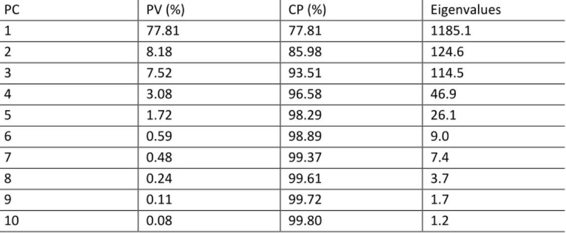
The PCA-DA algorithm was run on all the wavelengths (n = 1523) and the results indicated that the maximum variation was shown by the first principal component (PC1) with a cumulative proportion (CP) of 77.81% followed by PC2 (85.98%) with a proportion of variance (PV) of 8.18% (Table 2). The first ten PCs gave a cumulative proportion (CP) total of 99.80% (Table 2). The first 10 PCs were retained as the common
PCs. It can be noted that there is a decline in the eigenvalues from higher to lower order PCs (Table 2).
Table 2. Principal Component Analysis (PCA) results showing the proportion of variance (PV) and cumulative proportion (CP) in percentage (%) and eigenvalues for the first 10 principal components (PCs) of reflectance values from six urban tree species.
PC PV (%) CP (%) Eigenvalues 1 77.81 77.81 1185.1 2 8.18 85.98 124.6 3 7.52 93.51 114.5 4 3.08 96.58 46.9 5 1.72 98.29 26.1 6 0.59 98.89 9.0 7 0.48 99.37 7.4 8 0.24 99.61 3.7 9 0.11 99.72 1.7 10 0.08 99.80 1.2
The variable of importance in the projection (VIP) was used to determine the 10 best wavelengths with high scores. The significant wavelengths were selected from the 10 PCs with eigenvalues greater than 1.
The ten selected wavelengths using the PCA-DA had the highest VIP percentage values of 100% for both the Quercus spp. and Jacaranda mimosifolia (Figure 3). The lowest VIP percentage values were for Pinus spp. which ranged from 34% (1796) to 50% (2152) (Figure 3).
3.2 PLS-DA Wavelength Selection Results
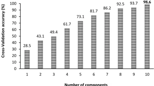
The PLS-DA model was applied on all the hyperspectral wavelengths (n = 1523) to select the important variables for the classification of the common urban trees. The optimal value used for the model was component number 10 (Figure 4) which had a CV accuracy value of 98.6%. This value increases with the number of components where 28.5% was obtained for the 1st component and 98.6% for the 10th component (Figure 4). The 10
principal components were used in developing the PLS-DA model in this study, and VIP scores for the individual wavelengths were calculated.
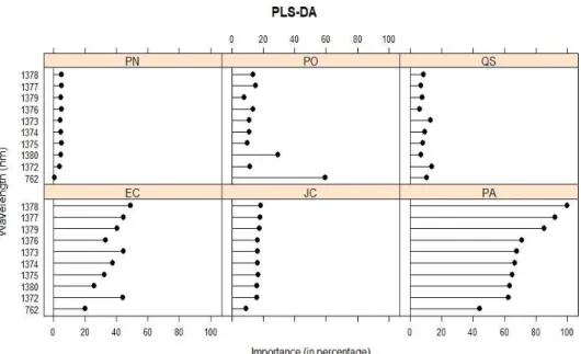
The ten wavelengths selected by the PLS-DA algorithm had low VIP percentage values for Pinus spp., with the highest being 5% for the 1378 nm, 1377 nm, 1376 nm and 1375 nm wavelengths (Figure 5). The highest VIP values for all the common urban trees wavelengths using the PLS-DA algorithm were obtained on the Platanus x acerifolia ranging from 44% (762 nm) to 100% (1378 nm) as shown in Figure 5.
Figure 3. Wavelengths selected using the VIP method for the six urban trees in this study using PCA-DA. The trees are Eucalyptus spp. (EC), Jacaranda mimosifolia (JC), Quercus spp. (QS), Platanus occidentalis (PO), Platanus x acerifolia (PA) and Pinus spp. (PN).
Figure 4. Discriminatory power for PLS-DA components using all hyperspectral wavelengths data (n = 1523). The 10-fold cross-validation resampling method was used to get cross-validation accuracy results for the components. The optimal component with the highest accuracy value is shown in bold. 28.5 43.1 49.4 61.7 73.1 81.7 86.2 92.5 93.7 98.6 0 10 20 30 40 50 60 70 80 90 100 1 2 3 4 5 6 7 8 9 10 Cr o ss -Val id ation ac cu rac y ( % ) Number of components
Figure 5. Wavelengths selected using the VIP method for the six common urban trees in this study using PLS-DA. The six common urban trees are Eucalyptus spp. (EC), Jacaranda mimosifolia (JC), Quercus spp. (QS), Platanus occidentalis (PO), Platanus x acerifolia (PA) and Pinus spp. (PN). 3.3 GRRF Wavelength Selection Results
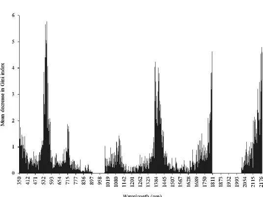
The RF method was utilised to select features that are most relevant to each other from the overall hyperspectral data (n = 1523) collected using the ASD field spectrometer. The mean decrease in Gini index was used to select the most important wavelengths in differentiating the common urban trees. The importance scores were derived using the mean decrease in Gini index. The mean decrease in Gini index values in the visible region (350–700 nm) ranged from 0.03 (595 nm) to 5.86 (587 nm) (Figure 6). The mean decrease in Gini values in the NIR region (700-1300 nm) were from 0 (885, 890, 898, 1171, 1199, 1203, 1206, 1208 and 1259, 1281 nm) to 1.86 (713 nm). The Red edge region (680-750 nm) had mean decrease in Gini index values ranging from 0.12 (690 nm) to 1.86 (713 nm). The mean decrease in index values in the SWIR (1300–2500 nm) ranged from 0 (1618 nm) to 5.29 (2174 nm) (2174 nm) (Figure 6).
The GRRF was used to select the important wavelengths from the importance scores obtained using the traditional RF classifier. The GRRF technique selected 13 optimal wavelengths where five wavelengths (360 nm, 409 nm, 513 nm, 562 nm, 618 nm) were in the visible region whilst the rest were in the SWIR region (Figure 7). These optimal wavelengths were then utilized as input variables in distinguishing common urban trees using the SVM and RF classification methods.
Figure 6. The mean decrease in Gini index showing the variable of importance for all the variables (n = 1523) for the traditional RF classifier. The important variables have a high mean decrease in Gini index value.
Figure 7. The wavelengths with the highest importance scores selected by the GRRF as calculated by the traditional RF for the urban trees.
0 1.5 3 4.5 360 409 513 562 618 1362 1380 1382 1384 1397 1660 1723 2122 Me an d ecre ase in Gini in d ex Wavelength in nanometers (nm)
3.4 Comparison of the Selected Wavelengths from the Three Feature Selection Techniques (PCA-DA, PLS-DA and GRRF)
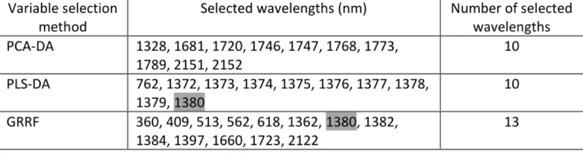
The wavelengths selected by the three feature selection techniques (PCA-DA, PLS-DA and GRRF are shown in Table 3. Both the PCA-DA and PLS-DA selected 10 wavelengths, while the GRRF selected 13 wavelengths from the total number of wavelengths (n = 1523) used in this study (Table 3). One wavelength (1380 nm) appeared in both the PLS-DA and GRRF, illustrating that it could potentially discriminate tree species using both feature selection techniques.
Table 3. Wavelengths selected by the PCA-DA, PLS-DA and GRRF techniques. The wavelength that was able to differentiate in both PLS-DA and GRRF is highlighted in grey.
Variable selection method
Selected wavelengths (nm) Number of selected wavelengths PCA-DA 1328, 1681, 1720, 1746, 1747, 1768, 1773, 1789, 2151, 2152 10 PLS-DA 762, 1372, 1373, 1374, 1375, 1376, 1377, 1378, 1379, 1380 10 GRRF 360, 409, 513, 562, 618, 1362, 1380, 1382, 1384, 1397, 1660, 1723, 2122 13 3.5 Accuracy Assessment
To ensure the stability of the model, the random splitting of the selected data into 70% for training and 30% for accuracy assessment was randomly repeated seven times. The accuracies were tested, and they showed no significant differences. The optimal wavelengths selected by PCA-DA (n = 10), PLS-DA (n = 10) and GRRF (n = 13) were classified using the SVM and the traditional RF classifier. As shown in Table 4, the SVM classifier had the highest overall accuracy values as compared to RF for all the feature selection techniques (PCA-DA, PLS-DA and GRRF). The GRRF produced the highest overall accuracy value (95.3%) with a kappa coefficient of 94.4% compared to the PCA-DA’s overall accuracy (86%) and kappa coefficient (83.2%) and PLS-DA’s overall accuracy (93.3%) and kappa coefficient (92%) using the SVM classifier (Table 4). The selected wavelengths using the GRRF technique also produced the highest overall accuracy value (88.7%) and kappa coefficient (86.4%) as compared to PCA-DA’s
accuracy value (64%) and kappa coefficient (56.8%) and PLS-DA’s accuracy value (72%) using the RF classifier (Table 5).
Table 4. Confusion matrix obtained using SVM classifier for the selected wavelengths using PCA-DA, PLS-DA and GRRF. The overall accuracy (OA) and kappa values are shown for the urban trees namely; Eucalyptus spp. (EC), Jacaranda mimosifolia (JC), Quercus spp. (QS), Platanus occidentalis (PO), Platanus x acerifolia (PA) and Pinus spp. (PN).
PCA-DA Class EC JC QS PO PA PN Total EC 20 2 1 0 0 0 23 JC 5 20 1 0 3 0 29 QS 0 0 22 1 2 0 25 PO 0 3 0 23 1 0 27 PA 0 0 1 1 19 0 21 PN 0 0 0 0 0 25 25 Total 25 25 25 25 25 25 150 OA = 86% Kappa = 83.2% PLS-DA Class EC JC QS PO PA PN Total EC 21 2 0 0 0 0 23 JC 2 23 0 1 0 0 26 QS 1 0 22 0 0 0 23 PO 0 0 1 24 0 0 25 PA 1 0 2 0 25 0 28 PN 0 0 0 0 0 25 25 Total 25 25 25 25 25 25 150 OA = 93.3% Kappa = 92% GRFF Class EC JC QS PO PA PN Total EC 24 0 1 0 0 0 25 JC 0 25 0 0 0 0 25 QS 1 0 23 0 1 0 25 PO 0 0 0 23 1 0 24 PA 0 0 1 2 23 0 26 PN 0 0 0 0 0 25 25 Total 25 25 25 25 25 25 150 OA = 95.3% Kappa = 94.4%
Table 5. Confusion matrix obtained using RF classifier for the selected wavelengths using PCA-DA, PLS-DA and GRRF. The overall accuracy (OA) and kappa values are shown for the urban trees namely; Eucalyptus spp. (EC), Jacaranda mimosifolia (JC), Quercus spp. (QS), Platanus occidentalis (PO), Platanus x acerifolia (PA) and Pinus spp. (PN).
PCA-DA Class EC JC QS PO PA PN Total EC 13 3 0 1 3 0 20 JC 6 13 3 0 6 0 28 QS 2 1 16 0 2 0 21 PO 2 5 3 17 2 0 29 PA 2 3 3 7 12 0 27 PN 0 0 0 0 0 25 25 Total 25 25 25 25 25 25 150 OA = 64% Kappa = 56.8% PLS-DA Class EC JC QS PO PA PN Total EC 14 1 0 0 0 0 15 JC 3 20 2 3 6 0 34 QS 0 0 22 4 0 0 26 PO 4 0 0 17 2 0 23 PA 4 4 1 1 17 0 27 PN 0 0 0 0 0 25 25 Total 25 25 25 25 25 25 150 OA = 76.7% Kappa = 72% GRFF Class EC JC QS PO PA PN Total EC 19 1 1 1 1 0 23 JC 1 23 0 0 0 0 24 QS 1 1 22 1 0 0 25 PO 1 0 2 20 1 0 24 PA 3 0 0 3 23 0 29 PN 0 0 0 0 0 25 25 Total 25 25 25 25 25 25 150 OA = 88% Kappa = 86.4%
Table 6 shows the PA and UA results from the selected wavelengths after being classified using the traditional RF classifier.
Table 6. Producer’s accuracy (PA) and user’s accuracy (UA) values for RF and SVM obtained from the optimal wavelengths selected using PCA-DA, PLS-DA and GRRF for the trees used in this study. The trees are Eucalyptus spp. (EC), Jacaranda mimosifolia (JC), Quercus spp. (QS), Platanus occidentalis (PO), Platanus x acerifolia (PA) and Pinus spp. (PN).
PCA-DA PLS-DA GRRF RF SVM RF SVM RF SVM Class PA UA PA UA PA UA PA UA PA UA PA UA EC 52 65 80 87 56 93 84 91 84 84 96 92 JC 52 46 80 69 80 59 92 88 88 88 100 100 PA 48 44 76 90 68 63 100 89 84 88 92 88 PO 68 59 92 85 68 74 96 96 84 78 92 96 QS 64 76 88 88 88 85 88 96 92 96 92 96 PN 100 100 100 100 100 100 100 100 100 100 100 100
4
DISCUSSION
There has been a wide use of field spectral data for discriminating and classifying trees. The results of this study show the ability of hyperspectral data in the classification of six urban trees in Randburg municipal area. This is in line with several studies: for example, Raczko and Zagajewski (2017) used hyperspectral data in mapping tree species in Poland; Cao et al. (2018) used field hyperspectral data in identifying eight
mangrove species in Qi’ao Island of Zhuhai, China. Adam and Mutanga (2009) and Mureriwa et al. (2016) used hyperspectral data in the spectral discrimination and classification of vegetation species in South Africa. Due to the huge data volume and high dimensionality of hyperspectral data, the removal of redundant data and identification of key wavelengths is vital for the classification of urban trees (Aval et al. 2019). Various techniques have been applied in reducing the high dimensionality of hyperspectral data and it is vital to minimize the loss of information.
In this study, it was difficult to use a single feature selection method as no technique has been universally proven to be superior over others in selecting the optimal wavelengths for the classification of vegetation species (Adam and Mutanga 2009). Hence three methods (PCA-DA, PLS-DA and GRRF) were used for feature selection and dimensionality reduction of field hyperspectral data. This is a key prerequisite for mapping urban tree species using remote sensing airborne and hyperspectral sensors as a small number of selected wavelengths give detailed information for classification purposes (Abbasi et al. 2019).
4.1 Classification Using Wavelengths Selected by Multispectral Statistical Techniques
Most of the optimal bands selected by the three feature selection techniques (PCA-DA, PLS-DA and GRRF) in classifying the urban trees (Eucalyptus spp., Jacaranda
mimosifolia, Platanus x acerifolia, Platanus occidentalis, Quercus spp.and Pinus spp.) were in the SWIR region. This is in line with other studies (Ferreira et al. 2015; Alonzo et al. 2014; Dalponte et al. 2012) which observed wavelengths in the SWIR region as the most suitable bands for classifying trees. The trees investigated here, are invasive and are of particular threat to water resources when found close or in waterways and riverbanks (Le Maitre et al. 2002; Henderson 2001). In the classification of tree species, the significance of the SWIR bands may be due to their capability in discriminating the subtle variations in the moisture content from one species’ type to the other
(Cherrington 2016). Although there were no biochemical features directly assessed in this study, it assumed that varying lignin and the amount of cellulose available in foliar and plant matter that is non-photosynthetic might have driven the separability of trees in the SWIR region (Alonzo et al. 2014).
None of the wavelengths was selected from the NIR region when the PCA-DA algorithm was applied. Only a single wavelength (762 nm) in the NIR region of the electromagnetic spectrum was selected by the PLS-DA algorithm. The results are in line with previous studies (Oldeland et al. 2017; Alonzo et al. 2014) who found the NIR region of less importance in discriminating tree species. Alonzo et al. (2014) used hyperspectral data to map 29 tree species (including the six tree species used in this study) in Santa Barbara, California, while Oldeland et al. (2017) classified 16 other tree and shrub species in central Namibia. Oldeland et al. (2017) found that the high variation within the classes and the reflectance might have been influenced by metabolites (e.g. proteins) and water resulting in the SWIR to play a critical role in discriminating tree species. The GRRF algorithm selected 5 significant wavelengths in the visible region, from 360 nm to 618 nm (Figure 7). The reflectance from the visible region in this study was mainly associated with the absorption traits of the trees’ leaf
pigments (Aval et al. 2019). These results also agree with those in the literature (Abbasi et al. 2019; Mureriwa et al. 2016) which showed a correlation between wavelength absorption in the visible region and leaf chlorophyll content in the tree leaves.
4.2 Comparison of the Selected Wavelengths from the Three Feature Selection Techniques (PCA-DA, PLS-DA and GRRF)
The wavelengths selected by PCA-DA (n = 10) were all in the SWIR region and showed high autocorrelation. The PLS-DA selected one wavelength (762 nm) in the NIR region and the rest (n = 9) in the SWIR region. The 9 wavelengths were from 1372 nm to 1380 nm showing high autocorrelation. The GRRF selected 5 wavelengths in the visible region, the rest (n = 8) were in the SWIR. The optimal wavelengths selected using GRRF achieved higher accuracies than the ones selected by PCA-DA and PLS-DA. The low classification accuracy from the wavelengths selected by PCA-DA and PLS-DA was due to high autocorrelation within the field spectral data where the prediction models’
performance was affected by the multicollinearity of the data due to continuous wavelengths (Adam and Mutanga 2009). The results obtained using the selected optimal wavelengths by the GRRF showed that the classifier’s prediction accuracy is
improved if correlated variables are removed. The GRRF achieved high classification accuracies due to its use of a selected subset of optimal wavelengths affirming its ability to choose vital wavelengths that enhance the performance of the classification models
(Mureriwa et al. 2016). The optimal wavelengths selected by the three feature selection techniques were put to comparison with wavelengths chosen in some previous studies (Table 7). The differences in the selected optimal wavelengths with previous studies can be attributed to differences in water content of leaves, differences in the concentration of pigments, biochemical leaf components and other characteristics that result in distinct interactions in the same wavelength region (Kumar et al. 2002).
Table 7. Wavelength regions, range and number of wavelengths as defined by (Kumar et al. 2002).
Region name Reference Optimal wavelengths selected (nm)
1. Visible (350-700 nm) Schmidt and Skidmore (2003)
404, 628 Adam and Mutanga (2009) No wavelength Abbasi et al. (2019) 363, 423
This study 360, 409, 513, 562, 618 2. Red edge (680-750
nm)
Schmidt and Skidmore (2003)
No wavelength Adam and Mutanga (2009) 745, 746 Abbasi et al. (2019) 721
This study No wavelength 3. Near-infrared (NIR)
(700-1300 nm)
Schmidt and Skidmore (2003)
771
Adam and Mutanga (2009) 892, 932, 934, 958, 961, 989 Abbasi et al. (2019) 1064, 1388
This study 762
4. Short-wave infrared (SWIR) (1300-2500 nm)
Schmidt and Skidmore (2003)
1398, 1803, 2183 Adam and Mutanga (2009) No wavelength Abbasi et al. (2019) No wavelength
This study 1328, 1362, 1372 to 1380, 1382, 1384, 1397, 1660, 1681, 1720, 1723, 1746, 1747, 1768, 1773, 1789, 2122, 2151, 2152
4.3 Comparison of Classification Algorithms
The performance of the RF and SVM classifiers was compared on the selected wavelengths by the feature selection techniques (PCA-DA, PLS-DA and GRRF). In previous studies (e.g. Brabant et al. 2019; Fassnacht et al. 2014; Dalponte et al. 2012), RF and SVM classifiers have been compared and yielded different results where some studies noted higher accuracy results for RF over SVM classifier, and vice versa. But this was not always upholding, others found SVM performing better than the RF classifier (Brabant et al. 2019; Ballanti et al. 2016; Fassnacht et al. 2014; Dalponte et al. 2012). Dalponte et al. (2012) found the SVM performing better than the RF classifier in mapping trees in the Southern Alps, which was likely due to the RF’s inability to handle
small training sample size. Moreover, Brabant et al. (2019) found SVM performing better than RF in comparing hyperspectral techniques in the classification of urban tree diversity in Toulouse, France. On the other hand, Sun et al. (2019) found the RF performing better than SVM and Artificial Neutral Network (ANN) in classifying high dimensional tropical dry forest using HyMap and Laser Vegetation Imaging Sensor (LVIS) in Costa Rica. In comparison to the RF classifier, SVM produced higher overall classification and kappa values in this study (Table 4). The performance of the SVM classifier in this study might have been due to its capability to classify with a small training dataset as the selected wavelengths for the feature selection techniques were 13 for GRRF and 10 for both PCA-DA and PLS-DA. The SVM classifier tends to perform better than RF if sample sizes are small, due to its ability to construct models based on support vectors derived from different classes, thereby maximizing the margin between the optimal hyperplane and the support vectors (Li et al. 2015).
In general, the optimal wavelengths selected by the three feature selection techniques (PCA-DA, PLS-DA and GRRF) concur with the band placement of several multispectral (e.g. Worldview-3 and Sentinel-2) and hyperspectral (e.g. Hyperion and Airborne Prism Experiment (APEX)) sensors (Brabant et al. 2019; Marcinkowska-Ochtyra et al. 2017; Li et al. 2015). However, the field spectrometer acquires data with less noise and has contiguous spectral wavelengths in comparison to broadbands acquired using the popular spaceborne and airborne sensors (Asner 1998). Passive space-borne sensors are affected by numerous sky conditions which include changes in the solar zenith angle and atmospheric interferences (e.g. clouds, dust and pollution) (Fitzgerald 2010). The above-mentioned shortcomings impede the utilization of passive spaceborne sensors in mapping urban tree species because they alter the quality and amount of the wavelength striking the tree leaves (Fitzgerald 2010). Further research is required to identify a suitable multispectral or hyperspectral image with low signal-to-noise ratio and less atmospheric interferences for mapping tree species over a large areal extent in the study area.
Overall, high accuracies achieved in this study demonstrate the potential of field spectral data in the classification of urban trees. The accurate classification of the urban trees is of paramount importance to municipalities and urban forest managers in the green space or urban forest management.
5
CONCLUSION
The focus of this study was to identify the key wavelengths for classifying urban trees (Eucalyptus spp., Jacaranda mimosifolia, Platanus x acerifolia, Platanus occidentalis, Quercus spp. and Pinus spp.) using feature selection methods on field hyperspectral data. Our main findings include: (1) The use of various feature selection techniques such as PCA-DA, PLS-DA and GRRF can reduce the high dimensionality associated with field hyperspectral data in a heterogeneous area (2) The selected wavelengths by GRRF produced high classification accuracies, followed by PLS-DA and lastly, PCA-DA feature selection methods. The selected wavelengths were classified using RF and SVM classification methods. The GRRF can be regarded as the most effective and efficient feature selection tool compared to PCA-DA and PLS-DA in reducing the high
dimensionality of field hyperspectral data. The selected key wavelengths were mainly in the SWIR region of the electromagnetic spectrum showing that they can be used to classify urban trees (3) The SVM classifier proved to be more reliable as compared to RF in classifying the selected wavelengths of the urban trees.
Overall, this study shows the potential of feature selection methods in reducing the high dimensionality and classification of urban trees using field hyperspectral data. Although this study was conducted using field hyperspectral data on urban trees with data collected using stratified purposeful sampling, the results do not show the spatial distribution of the species in the whole study area. The use of very high spatial resolution (VHSR) hyperspectral images such as Airborne Prism Experiment (APEX) and Hyperion or multispectral images such as Worldview and Sentinel-2 can assist in providing information on the spatial distribution of the urban trees in the study area which can be of great importance to the municipality and stakeholders involved in greenspace or urban tree management.
REFERENCES
Abbasi, M., Verrelst, J., Mirzaei, M., Marofi, S. and Riyahi Bakhtiari, H.R. (2019) Optimal Spectral Wavelengths for Discriminating Orchard Species Using Multivariate Statistical Techniques. Remote Sensing, 12, 63
Abiye, T. (2015) The Role of Wetlands Associated to Urban Micro-Dams in Pollution Attenuation, Johannesburg, South Africa. Wetlands, 35, 1127-1136
Adam, E. and Mutanga, O. (2009) Spectral discrimination of papyrus vegetation (Cyperus papyrus L.) in swamp wetlands using field spectrometry. ISPRS Journal of Photogrammetry and Remote Sensing, 64, 612-620
Almeida, A.M. and Tomé, M. (2009) Field sampling of cork value before extraction in
Portuguese ‘montados’. Agroforestry systems, 79, 419-430
Alonzo, M., Bookhagen, B. and Roberts, D.A. (2014) Urban tree species mapping using hyperspectral and lidar data fusion. Remote Sensing of Environment, 148, 70-83
Asner, G.P. (1998) Biophysical and biochemical sources of variability in canopy reflectance. Remote Sensing of Environment, 64, 234-253
Aval, J., Fabre, S., Zenou, E., Sheeren, D., Fauvel, M. and Briottet, X. (2019) Object-based fusion for urban tree species classification from hyperspectral, panchromatic and nDSM data. International Journal of Remote Sensing, 40, 5339-5365 Ballanti, L., Blesius, L., Hines, E. and Kruse, B. (2016) Tree species classification using
hyperspectral imagery: A comparison of two classifiers. Remote Sensing, 8, 445
Barker, M. and Rayens, W. (2003) Partial least squares for discrimination. Journal of Chemometrics, 17, 166-173
Bartesaghi-Koc, C., Osmond, P. and Peters, A. (2019) Mapping and classifying green infrastructure typologies for climate-related studies based on remote sensing data. Urban Forestry & Urban Greening, 37, 154-167
Brabant, C., Alvarez-Vanhard, E., Laribi, A., Morin, G., Thanh Nguyen, K., Thomas, A. and Houet, T. (2019) Comparison of Hyperspectral Techniques for Urban Tree Diversity Classification. Remote Sensing, 11, 1269.
Breiman, L. (2001) Random forests. Machine learning, 45, 5-32
Calviño-Cancela, M. and Martín-Herrero, J. (2016) Spectral Discrimination of Vegetation Classes in Ice-Free Areas of Antarctica. Remote Sensing, 8, 856 Cao, J., Liu, K., Zhu, Y., Li, J. and He, Z. (2018) Identifying Mangrove Species Using Field
Close-Range Snapshot Hyperspectral Imaging and Machine-Learning Techniques. Remote Sensing, 10, 2047
Cherrington, E.A. (2016) Towards ecologically consistent remote sensing mapping of tree communities in French Guiana. PhD Thesis, Technische Universität Dresden
Chivasa, W., Mutanga, O. and Biradar, C. (2019) Phenology-based discrimination of maize (Zea mays L.) varieties using multitemporal hyperspectral data. Journal of Applied Remote Sensing, 13, 017504
Cocchi, M., Biancolillo, A. and Marini, F. (2018) Data Analysis for Omic Sciences: Methods and Applications, pp. 265-299
Dalponte, M., Bruzzone, L. and Gianelle, D. (2012) Tree species classification in the Southern Alps based on the fusion of very high geometrical resolution multispectral/hyperspectral images and LiDAR data. Remote Sensing of Environment, 123, 258-270
de Santana, F.B., Borges Neto, W. and Poppi, R.J. (2019) Random forest as one-class classifier and infrared spectroscopy for food adulteration detection. Food Chem, 293, 323-332
Degerickx, J., Roberts, D.A. and Somers, B. (2019) Enhancing the performance of Multiple Endmember Spectral Mixture Analysis (MESMA) for urban land cover mapping using airborne lidar data and band selection. Remote Sensing of Environment, 221, 260-273
Deng, H. and Runger, G. (2013) Gene selection with guided regularized random forest. Pattern Recognition, 46, 3483-3489
Dizdaroglu, D., Yigitcanlar, T. and Dawes, L. (2009) Sustainable urban futures : an ecological approach to sustainable urban development. https://eprints.qut. edu.au/29539/1/c29539.pdf
Farrugia, B. (2019) WASP (write a scientific paper): Sampling in qualitative research. Early Hum Dev, 133, 69-71
Fassnacht, F.E., Latifi, H., Stereńczak, K., Modzelewska, A., Lefsky, M., Waser, L.T.,
Straub, C. and Ghosh, A. (2016) Review of studies on tree species classification from remotely sensed data. Remote Sensing of Environment, 186, 64-87 Fassnacht, F.E., Neumann, C., Forster, M., Buddenbaum, H., Ghosh, A., Clasen, A., Joshi,
P.K. and Koch, B. (2014) Comparison of Feature Reduction Algorithms for Classifying Tree Species With Hyperspectral Data on Three Central European Test Sites. IEEE Journal of Selected Topics in Applied Earth Observations and Remote Sensing, 7, 2547-2561
Ferreira, M.P., Zortea, M., Zanotta, D.C., Féret, J.B., Shimabukuro, Y.E. and Souza Filho, C.R. (2015) On the Use of Shortwave Infrared for Tree Species Discrimination in Tropical Semideciduous Forest. ISPRS - International Archives of the
Photogrammetry, Remote Sensing and Spatial Information Sciences, XL-3/W3, 473-476
Fitzgerald, G.J. (2010) Characterizing vegetation indices derived from active and passive sensors. International Journal of Remote Sensing, 31, 4335-4348
Foody, G.M. and Mathur, A. (2004) A relative evaluation of multiclass image classification by support vector machines. IEEE Transactions on Geoscience and Remote Sensing, 42, 1335-1343
Forsyth, G., Richardson, D., Brown, P. and Van Wilgen, B. (2004) A rapid assessment of the invasive status of Eucalyptus species in two South African provinces: working for water. South African Journal of Science, 100, 75-77
Ghiyamat, A., Shafri, H.Z.M., Amouzad Mahdiraji, G., Shariff, A.R.M. and Mansor, S. (2013) Hyperspectral discrimination of tree species with different classifications using single- and multiple-endmember. International Journal of Applied Earth Observation and Geoinformation, 23, 177-191
Gholizadeh, H., Gamon, J.A., Zygielbaum, A.I., Wang, R., Schweiger, A.K. and Cavender-Bares, J. (2018) Remote sensing of biodiversity: Soil correction and data
dimension reduction methods improve assessment of α-diversity (species richness) in prairie ecosystems. Remote Sensing of Environment, 206, 240-253 Ginsburg, S.B., Viswanath, S.E., Bloch, B.N., Rofsky, N.M., Genega, E.M., Lenkinski, R.E. and Madabhushi, A. (2015) Novel PCA-VIP scheme for ranking MRI protocols and identifying computer-extracted MRI measurements associated with central gland and peripheral zone prostate tumors. J Magn Reson Imaging, 41, 1383-1393
Guyon, I., Andr, #233 and Elisseeff (2003) An introduction to variable and feature selection. J. Mach. Learn. Res., 3, 1157-1182
Henderson, H. (1990) Jacaranda. Farming in South Africa. Weeds A, 30, 2132-2134. Henderson, L. (2001) Alien weeds and invasive plants: A complete guide to declared
weeds and invaders in South Africa, Plant Protection Research Institute, Pretoria, South Africa
Henry, A. and Flood, M.G. (1919) The history of the London plane, Platanus acerifolia, with notes on the genus Platanus. Proceedings of the Royal Irish Academy. Section B: Biological, Geological, and Chemical Science. https://www. jstor.org/stable/pdf/20517052.pdf?refreqid=excelsior%3A9448762d0215ab a2168bd83f10be79de
Izquierdo-Verdiguier, E., Zurita-Milla, R. and Rolf, A. (2017) On the use of guided regularized random forests to identify crops in smallholder farm fields. 2017 9th International Workshop on the Analysis of Multitemporal Remote Sensing Images (MultiTemp).
https://ieeexplore.ieee.org/stamp/stamp.jsp?tp=&arnumber=8035248
Jarocińska, A., Białczak, M. and Sławik, Ł. (2018) Application of aerial hyperspectral
images in monitoring tree biophysical parameters in urban areas. Miscellanea Geographica, 22, 56-62
Jombo, S., Adam, E., Byrne, M.J. and Newete, S.W. (2020) Evaluating the capability of Worldview-2 imagery for mapping alien tree species in a heterogeneous urban environment. Cogent Social Sciences, 6, 1754146
Jovanovic, G., Romanic, S.H., Stojic, A., Klincic, D., Saric, M.M., Letinic, J.G. and Popovic, A. (2019) Introducing of modeling techniques in the research of POPs in breast milk - A pilot study. Ecotoxicol Environ Saf, 172, 341-347
Karlson, M., Ostwald, M., Reese, H., Bazié, H.R. and Tankoano, B. (2016) Assessing the potential of multi-seasonal WorldView-2 imagery for mapping West African agroforestry tree species. International Journal of Applied Earth Observation and Geoinformation, 50, 80-88
Kiala, Z., Mutanga, O., Odindi, J. and Peerbhay, K. (2019) Feature Selection on Sentinel-2 Multispectral Imagery for Mapping a Landscape Infested by Parthenium Weed. Remote Sensing, 11
Kumar, L., Schmidt, K., Dury, S. and Skidmore, A. (2002) Imaging spectrometry, pp. 111-155, Springer
Le Maitre, D.C., van Wilgen, B.W., Gelderblom, C.M., Bailey, C., Chapman, R.A. and Nel, J.A. (2002) Invasive alien trees and water resources in South Africa: case studies of the costs and benefits of management. Forest ecology and management, 160, 143-159
Lee, L.C., Liong, C.Y. and Jemain, A.A. (2018) Partial least squares-discriminant analysis (PLS-DA) for classification of high-dimensional (HD) data: a review of contemporary practice strategies and knowledge gaps. Analyst, 143, 3526-3539
Li, D., Ke, Y., Gong, H. and Li, X. (2015) Object-based urban tree species classification using bi-temporal WorldView-2 and WorldView-3 images. Remote Sensing, 7, 16917-16937
Li, X., Chen, W.Y., Sanesi, G. and Lafortezza, R. (2019) Remote Sensing in Urban Forestry: Recent Applications and Future Directions. Remote Sensing, 11, 1144
Liu, L., Coops, N.C., Aven, N.W. and Pang, Y. (2017) Mapping urban tree species using integrated airborne hyperspectral and LiDAR remote sensing data. Remote Sensing of Environment, 200, 170-182
Love, S.L., Wimpfheimer, R. and Noble, K. (2009) Selecting, planting, and caring for trees, shrubs, and vines, University of Idaho Extension
Malvern Panalytical (2019) ASD FieldSpec 4 Standard-Res Spectroradiometer
Marcinkowska-Ochtyra, A., Zagajewski, B., Ochtyra, A., Jarocińska, A., Wojtuń, B.,
Rogass, C., Mielke, C. and Lavender, S. (2017) Subalpine and alpine vegetation classification based on hyperspectral APEX and simulated EnMAP images. International Journal of Remote Sensing, 38, 1839-1864
Masetic, Z. and Subasi, A. (2016) Congestive heart failure detection using random forest classifier. Computer Methods and Programs in Biomedicine, 130, 54-64 Mountrakis, G., Im, J. and Ogole, C. (2011) Support vector machines in remote sensing:
A review. ISPRS Journal of Photogrammetry and Remote Sensing, 66, 247-259 Mureriwa, N., Adam, E., Sahu, A. and Tesfamichael, S. (2016) Examining the Spectral Separability of Prosopis glandulosa from Co-Existent Species Using Field Spectral Measurement and Guided Regularized Random Forest. Remote Sensing, 8, 144