Hunting For Metamorphic JavaScript Malware

(1)

San Jose State University

SJSU ScholarWorks

Master's Projects Master's Theses and Graduate Research

Spring 2014

Hunting For Metamorphic JavaScript Malware

Mangesh Musale

San Jose State University

Follow this and additional works at:https://scholarworks.sjsu.edu/etd_projects Part of theComputer Sciences Commons

This Master's Project is brought to you for free and open access by the Master's Theses and Graduate Research at SJSU ScholarWorks. It has been accepted for inclusion in Master's Projects by an authorized administrator of SJSU ScholarWorks. For more information, please contact [email protected].

Recommended Citation

Musale, Mangesh, "Hunting For Metamorphic JavaScript Malware" (2014).Master's Projects. 359. DOI: https://doi.org/10.31979/etd.ky84-3b5q

(2)

Hunting For Metamorphic JavaScript Malware

A Project Presented to

The Faculty of the Department of Computer Science San Jose State University

In Partial Fulfillment

of the Requirements for the Degree Master of Science

by

Mangesh Musale May 2014

(3)

c

○2014

(4)

The Designated Project Committee Approves the Project Titled

Hunting For Metamorphic JavaScript Malware

by

Mangesh Musale

APPROVED FOR THE DEPARTMENTS OF COMPUTER SCIENCE

SAN JOSE STATE UNIVERSITY

May 2014

Dr. Mark Stamp Department of Computer Science Dr. Thomas Austin Department of Computer Science Dr. Sami Khuri Department of Computer Science

(5)

ABSTRACT

Hunting For Metamorphic JavaScript Malware by Mangesh Musale

Internet plays a major role in the propagation of malware. A recent trend is the infection of machines through web pages, often due to malicious code inserted in JavaScript. From the malware writer’s perspective, one potential advantage of JavaScript is that powerful code obfuscation techniques can be applied to evade de-tection. In this research, we analyze metamorphic JavaScript malware. We compare the effectiveness of several static detection strategies and we quantify the degree of morphing required to defeat each of these techniques.

(6)

ACKNOWLEDGMENTS

I am very thankful to my advisor Dr. Mark Stamp for his continuous guidance and support throughout this project and believing me. Also, I would like to thank the committee members Dr. Thomas Austin and Dr. Sami Khuri for monitoring the progress of the project and their valuable time.

(7)

TABLE OF CONTENTS CHAPTER 1 Introduction . . . 1 2 Background . . . 3 2.1 Encrypted Malware . . . 3 2.2 Polymorphic Malware . . . 4 2.3 Metamorphic Malware . . . 4 2.3.1 Subroutines Permutation . . . 4 2.3.2 Instruction Reordering . . . 5 2.3.3 Instruction Substitution . . . 6 2.3.4 Register Swapping . . . 6

2.3.5 Garbage Instruction Insertion . . . 6

2.4 Detection Techniques . . . 7

2.4.1 Signature Based Detection . . . 7

2.4.2 Machine Learning Based Detection . . . 7

2.4.3 Opcode Graph Based Detection . . . 8

2.4.4 Simple Substitution Based Detection . . . 8

3 Transcriptase . . . 9

3.1 Instruction Permutation . . . 10

3.2 Variable/Function Name Randomization . . . 11

3.3 Meta Language Symbols . . . 12

(8)

3.5 Miscellaneous Challenges . . . 13

4 Rhino . . . 14

4.1 Architecture . . . 14

4.2 Modification . . . 17

5 Statistical Malware Detection . . . 20

5.1 Hidden Markov Model Method . . . 20

5.1.1 Markov Chain . . . 20

5.1.2 Hidden Markov Model . . . 21

5.1.3 HMM Implementation . . . 24

5.1.4 Log Likelihood Per Opcode . . . 24

5.2 Opcode Graph Similarity . . . 25

5.2.1 Opcode Graph . . . 25

5.2.2 Similarity Calculation . . . 27

5.2.3 Implementation . . . 28

5.3 Simple Substitution Distance . . . 28

5.3.1 Jakobsen Algorithm . . . 29

5.4 Singular Value Decomposition . . . 34

5.4.1 Algorithm . . . 34

6 Experiments . . . 38

6.1 Receiver Operating Characteristics . . . 39

(9)

6.3 Opcode Graph Similarity Method . . . 41

6.4 Simple Substitution Distance Method . . . 42

6.5 Singular Value Decomposition Method . . . 44

7 Enhancement . . . 46

7.1 Hidden Markov Model . . . 46

7.2 Opcode Graph Similarity Method . . . 48

7.3 Simple Substitution Distance Method . . . 48

7.4 Singular Value Decomposition Method . . . 50

8 Conclusion and Future Work . . . 52

APPENDIX ROC curves . . . 57

A.1 Hidden Markov Model . . . 57

A.2 Opcode Graph Similarity Method . . . 62

A.3 Simple Substitution Distance Method . . . 67

(10)

LIST OF TABLES

1 Opcode Sequence . . . 26

2 Digram Count Matrix . . . 26

3 Digram Probability Matrix . . . 27

4 Opcode Mapping (Putative Key) . . . 31

5 Key Before Swapping . . . 32

6 Key After Swapping . . . 32

7 D Matrix before Swapping . . . 32

8 D Matrix after Swapping . . . 33

9 Machine Specifications . . . 38

10 Source of Benign Files . . . 39

11 Simple Substitution Method Scores . . . 43

12 AUC for Hidden Markov Model . . . 47

13 AUC for Opcode Graph Similarity Method . . . 48

14 AUC for Simple Substitution Distance Method . . . 49

(11)

LIST OF FIGURES

1 Rhino Block Diagram . . . 15

2 Abstract Syntax Tree . . . 17

3 Sample Compilation Without Modification . . . 19

4 Sample Compilation With Modification . . . 19

5 Example of HMM . . . 21

6 Markov Process . . . 23

7 SVD Process . . . 37

8 HMM Score Analysis (N=2) . . . 40

9 ROC curve for HMM . . . 41

10 Opcode Graph Similarity Analysis . . . 42

11 ROC curve for Opcode Graph Similarity Method . . . 42

12 Simple Substitution Method Scores Analysis . . . 43

13 ROC for Simple Substitution Method . . . 44

14 SVD Scatter Plot Analysis . . . 45

15 ROC curve for SVD . . . 45

16 Hidden Markov Model AUC Analysis . . . 47

17 Opcode Graph Similarity Method AUC Analysis . . . 49

18 Simple Substitution Distance Method AUC Analysis . . . 50

19 Singular Value Decomposition AUC Analysis . . . 50

A.20 ROC for 2500 Functions for HMM . . . 57

(12)

(13)

A.46 ROC for 100 Functions for OGS . . . 62

(14)

A.70 ROC for 5000 Functions for SSM . . . 67

(15)

A.92 ROC for 100 Functions for SVD . . . 71

(16)

(17)

(18)

CHAPTER 1 Introduction

Internet has evolved into the greatest medium of communication and data ex-change that the world has ever known. Since its inception, the Internet has matured from just an academic experiment into an effective communication system. Since the late 1990s, it has became a vast interconnected source of information and services widely used for commercial and personal purposes. This evolution has led to the emergence of social networking, online banking and advertising, among various other commercial and non-commercial uses.

Transactions over the Internet often involve the transfer of sensitive data which attackers like to tap and exploit. For example, bank account information, medical records and passwords are routinely transferred over the network. Unfortunately, user’s personal computer is a weak link in this system wherein personal computers typically run a large number of applications which are rarely managed properly. Single visit to a compromised web page is sufficient to infect a web browser, particularly the one that has not been updated with recent security patches.

Web browsers are often infected through malicious code inserted into legitimate JavaScript on a website [24]. When a user visits such a compromised website, these malicious JavaScript programs are automatically loaded with HTML code in the web browser. Execution of such malicious JavaScript can expose the personal data of the user. The majority of malicious JavaScript redirects the web browser to load more malicious content from a remote server. This can be achieved through several means, such as adding an HTML iframe element to a page [19]. While there are relatively

(19)

few ways to obfuscate HTML code [35], JavaScript makes it possible by providing a vast array of methods to hide the payload.

In this research, we analyze a metamorphic JavaScript malware that is designed to infect other JavaScript files in the same folder. We consider a variety of static detection techniques and quantify the effectiveness of each. We also measure the degree of morphing required to defeat each of these detection strategies.

This paper is organized as follows. In Chapter 2, we provide background infor-mation on malware with an emphasis on metamorphic malware. Chapter 3 outlines the specific metamorphic JavaScript malware that forms the basis for the research in this paper. Then in Chapter 4, we cover the Rhino JavaScript engine and dis-cuss the modifications required for our experiments. Next, we disdis-cuss four different metamorphic detection techniques that we apply to the metamorphic JavaScript de-tection problem. Specifically, we consider Hidden Markov Model, an Opcode Graph similarity method, a distance measure inspired by Simple Substitution Cryptanaly-sis, and Singular Value Decomposition. These topics are covered in Chapter 5. Our experimental results for the original metamorphic JavaScript appear in Chapter 6. We consider an enhanced metamorphic JavaScript malware in Chapter 7 and provide the experimental results for this challenging case. Chapter 8 contains our conclusions and a consideration for future work.

(20)

CHAPTER 2 Background

Malware is a software program designed to do malicious activities on a user’s computer with the intention of extracting information and exploiting resources with-out his consent. Such programs either stop normal execution of benign programs or they start executing along with benign code to do malicious activities. They de-stroy files by infecting them or by deleting them, stealing sensitive user information. According to the execution pattern and internal structure, malicious softwares are categorized as follows:

2.1 Encrypted Malware

Signature detection is one of the trivial methods for malware detection in which, a pattern of bytes or instruction sequence is extracted as a signature of that particular malware. Then, every file is compared against the extracted signatures to check whether a given file is a malware or a benign file. To overcome this detection method, malware writers came up with Encrypted Malware. In such a type of malware, the entire body of malware is encrypted by using one of the encryption techniques. Code to decrypt this encrypted malware is also attached to its body. As a result of this, signature based detection method is unable to find a pattern in the file and decryption code will decrypt the malware at the time of execution, which will not affect the normal execution of malware. Cascade was the first virus of this kind which appeared in 1987 [20].

(21)

2.2 Polymorphic Malware

As the decryption code is not encrypted in Encrypted Malware, antivirus writers were able to extract the pattern from decryption code. The need to hide decryption code gave birth to Polymorphic Malware. In Polymorphic Malware, code to decrypt malware is morphed after every infection. Morphing is done in such a way that the internal structure of code gets changed completely without any change in the functionality [20]. This makes signature extraction hard. First polymorphic virus named 1260 was developed by Washburn in 1990 [28].

2.3 Metamorphic Malware

Metamorphic Malware is an advanced version of Polymorphic Malware. In this malware, internal structure of the malware gets changed after every execution. But the overall functionality remains the same [16]. There are various methods by which this can be achieved. Let us discuss a few of them.

2.3.1 Subroutines Permutation

Function definition can be inserted between any two statements in the code. Using this feature, malware writers reorder the function definitions, keeping the order of function call unique. This will give structurally different but functionally same software. Suppose, we have 𝑛 different functions in the code, then these functions can be arranged in 𝑛! different ways. This gives 𝑛! different morphed versions of the same code. Metamorphic malware such as win32/Ghost has used this type of subroutine permutation technique [37].

(22)

2.3.2 Instruction Reordering

In this method, independent instructions are reordered in a program scope. Here, independent instructions refer to those instructions whose execution does not depend on any previous instruction. This reordering will give us quite a large number of morphed versions of the same code [20]. If we have 𝑛independent instructions in the scope of a program, then we can generate 𝑛! different morphed versions. Illustrated below is a simple example of addition of two numbers.

1: int a = 10; 2: int b = 20; 3: int c = a + b ;

Here in statements 1 and 2, we declare two variables a, b and assign them constant values 10 and 20 respectively. Declaring a variable does not depend on any other statement. Therefore, in this example, statement 1 and 2 are independent instructions which can be arranged in any order. But, statement 3 depends on statement 1 and 2. Statement 3 adds two variables a and b, but to add them they must be declared and assigned some value. Therefore, statement 3 must appear after statement 1 and 2. Considering all these dependencies, the above code can be reordered to achieve the same functionality as shown below.

2: int b = 20; 1: int a = 10; 3: int c = a + b ;

(23)

2.3.3 Instruction Substitution

In this method, morphed copies are generated by replacing an instruction or a group of instructions by a functionally equivalent instruction or group of instruc-tions [32]. For example,

SUB EBX EBX can be replaced as

AND EBX 0x0000

SUB instruction subtracts the content of register B from the register B itself i.e., the code wants to clear register B. Same effect can be achieved through bitwise multipli-cation of register B contents with zero.

2.3.4 Register Swapping

In this method, morphed copies are generated by changing registers used in the instructions. This is a very simple way of code obfuscation. Win95/Regs wap [29] malware is such a kind of malware. Consider an example where we want to fetch the value from stack and load it into one of the registers for the next operation. POP EAX can be replaced with POP EBXif EBXregister is free at this moment. One of the drawbacks of this method is it does not alter the opcode sequence.

2.3.5 Garbage Instruction Insertion

In this method, morphed copies of malware are created by inserting instructions in software which will not affect execution [6]. Such ‘do-nothing’ instructions are used in creating morphed copies of malware such as Win95/ZPerm [29]. Examples of such instructions are NOP instruction or ADD EBX 0. Instructions like INC and DEC can be used in succession to increase the value in one of the registers and bring it back to

(24)

original.

2.4 Detection Techniques

There are several techniques to detect a malware. Different characteristics of malware are used in detection techniques such as statistical analysis on opcodes, pattern matching of bytes for a particular malware family. Some of the popular techniques are mentioned below:

2.4.1 Signature Based Detection

In this technique, content of malware is compared against the signature dictio-nary to check whether the given file is malware or benign. A dictiodictio-nary for known malware signatures is maintained and updated by anti-virus vendors. A signature is an algorithm or hash (a number derived from a string of text) that uniquely identifies a specific virus. Depending on the type of scanner being used, it may be a static hash, which in its simplest form, is a calculated numerical value of a snippet of code unique to the virus.

2.4.2 Machine Learning Based Detection

Machine learning is a very widely used concept in computer science. Hidden Markov Model (HMM) is one of the most popular machine learning techniques used to detect malware [27]. In this technique, a HMM is trained against known malware opcode sequence. This trained model is used to score files to be analyzed. If the score is more than a predefined threshold, then it is fairly good to say that the given file belongs to a malware family.

(25)

2.4.3 Opcode Graph Based Detection

In this technique, a digram frequency graph is constructed from opcode sequence of known malware. Similar graph is constructed for the file to be analyzed. Score of this file is calculated by taking absolute difference between corresponding elements in the graph. Lesser the score, higher is the probability of the file being a malware [22]. We will discuss more about this technique in Section 5.2.

2.4.4 Simple Substitution Based Detection

This technique is based on the assumption that frequency distribution of opcodes hold true to a certain extent for every malware family. In this technique, a digram frequency graph is constructed from an opcode sequence of a known malware and the file to be analyzed. A frequency count is taken for each unique opcode in the known malware. Frequency distribution of opcodes from known malware samples is mapped with frequency distribution of opcodes from files which are to be tested. The score for each file is calculated by the same method used in Jakobsen’s algorithm for Simple Substitution Cryptanalysis [13]. If the score for a file is less than a precalculated threshold, then it is reasonable to conclude that the file belongs to a malware family. Implementation details for this method are described in Section 5.3.

(26)

CHAPTER 3 Transcriptase

Transcriptase malware was originally designed by Sperl [25]. Transcriptase is a metamorphic malware implemented in JavaScript. Execution of this script infects all the JavaScript files in the folder where the malware script is placed. As a result of this infection, a morphed version of the malware script gets attached to benign JavaScript files in the folder. Whenever this infected JavaScript gets executed in any other folder, it infects other benign JavaScript files. For each infection, malware script generates a new morphed version. The malware script carries its code in a custom designed meta-language.

The morphing scheme used in this malware helps to evade signature based de-tection method. The meta-language code here is compiled using a compiler written in JavaScript. Compiler code is also a part of the malware body. Advantage of defin-ing a custom meta-language is that the malware writer can add extra information required to create the morphed versions. The general syntax used for an instruction in this malware sample is shown below

(Identifier |Restrictions) meta-instruction

Identifier and Restrictions are used by the permutation function for code obfuscation. Identifier is the unique identification for a statement in the script and Restriction is a list of statements which must be executed before the given statement. Details of this scheme is described in Section 3.1. These meta-instructions are used to create actual instructions in the script. Compiler creates a new malicious JavaScript in three steps as shown below:

(27)

∙ Permutation and Variable/Function-Name Randomization

∙ Code Creation

∙ Variable/Function Insertion

3.1 Instruction Permutation

In this part of the code, compiler parses the meta language code, scope by scope and collects all the information about instructions and their corresponding restric-tions. It analyzes the code in the given scope and starts permuting instructions considering their dependencies. For example, consider the following code

Here, first number is the identifier for the instruction. This remains unique in the entire JavaScript. Numbers after ‘|’ indicate dependencies of the given instruction. Instruction with identifier 200 does not have any number after ‘|’, shows that it does not depend on any other instruction. Instruction 200 is var b = 0. This is declaration of variable and assigns it a value 0. To declare a variable and assign it some constant value does not have any dependency on previous instructions.

But if we look at instruction 400,c + 1(b), to execute this instruction we need the value of variableb. Variableb is declared and assigned a value at instruction200. Therefore,200 appears in instruction 400 after ‘|’ to indicate dependency.

(28)

Permutation function reads this information and uses it to rearrange the instruc-tion. As we observe, there is no number after ‘|’ in instructions 100, 200 and 300, it means that these instructions are independent of any other instructions in the script. So, they can be rearranged as

Here, we changed the order of instructions as 300, 100, 200 without any effect on the functionality of the script. These three independent instructions can be arranged in 3! different ways. Due to the fast growth-rate of the permutation function, this technique is very useful in case of large number of instructions.

3.2 Variable/Function Name Randomization

The compiler searches for keywords likevar,defandfunctionin all instructions of the script. Then it gets the hard coded strings used to define them and replaces them with random strings. It then replaces all occurrences of these hard-coded strings in the current scope with the newly generated random string. For example, consider the following function definition.

f u n c t i o n m a k e S q u a r e ( n u m b e r ){ r e t u r n n u m b e r * n u m b e r ;} var num =1;

(29)

Compiler searches forvar,defandfunctionkeywords. Here, it will findmakeSquare, number, numand sqrvariable names. Then it will generate random strings and map each string with one variable name and replace it in the current scope. After that, it will search for the same variable name in upper scopes till the global scope is reached. After this step, the new form of code will be

f u n c t i o n p k j u o l e d r b n x ( q e r d s l d s ){ r e t u r n q e r d s l d s * q e r d s l d s ;} var h x e d l k e r d = 1;

def c a d w k g d = p k j u o l e d r b n x ( h x e d l k e r d );

3.3 Meta Language Symbols

After permutation of instructions and function/variable name randomization, the compiler parses the meta-language code and derives a valid JavaScript statement for every statement in meta-language. While deriving the actual instruction, several meta-language symbols are processed each having a special meaning. Compiler inter-prets them at runtime and generates appropriate javascript literals. For instance: var n u m b e r = # n1n #;

var str = # " H e l l o _ W o r l d " #; var exp = # x n t r u e n x #;

Here, #n...n# is interpreted as the value at position ... is a numerical value and #"..."# is interpreted as the value at position ... is a string value. Furthermore, #xn ... nx# is interpreted as the value at ... is a JavaScript literal like true or false, where 𝑛 can be any integer. At this step, each symbol is replaced with original JavaScript language literal.

(30)

3.4 Variables/Functions Insertion

During the compilation, many variables and functions are defined (either due to the meta-code itself, or due to obfuscation). They are not yet placed in the code, but are saved in special arrays. At the end of the code creation, they are placed in the code. Functions can be inserted between any two instructions in the global scope. Variables can be inserted between any two instructions in the current scope before they get used for the first time. This insertion takes a long time because the whole code has to be analyzed several times to find potential positions [17].

3.5 Miscellaneous Challenges

At the time of code creation, the compiler creates random functions. These functions perform arithmetic calculations and return integer values between0to255. They are then used to represent ASCII values of characters to derive strings. This makes the code highly obfuscated.

Compiler creates an array of functions. Use of this array of functions in con-structing strings makes the code highly unreadable. It is very hard to read and understand such a code in one parse [17].

(31)

CHAPTER 4 Rhino

In 1997, Netscape started working on a project to bring about a version of Netscape Navigator developed fully in Java. For this, they came up with a JavaScript engine which was also developed in Java. This JavaScript engine was named as the Rhino Project which is now maintained by Mozilla [21]. Rhino compiles JavaScript into Java classes and can operate in two modes—compiled mode and interpreted mode. In compiled mode, Rhino first compiles JavaScript and then converts it into Java bytecode. Then this bytecode can be run as a Java program. This improves the execution time of JavaScript.

4.1 Architecture

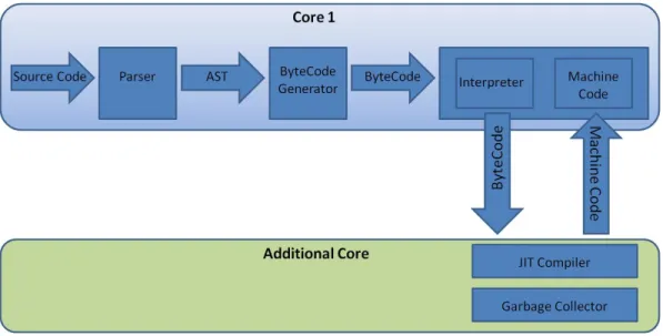
Rhino JavaScript Engine consists of four basic building blocks—Parser, Byte-Code Generator, Interpreter and JIT. The JavaScript source code is first fed to a Parser which parses the code and converts it into an Abstract Syntax Tree (AST). Then this AST is fed to the ByteCode Generator which generates the bytecode. This bytecode is used by the Rhino Interpreter which converts it into machine code with the help of JIT. Finally, this machine code gets executed [33]. Block diagram of Rhino JavaScript Engine can be visualized in Figure 1.

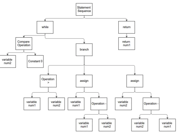
Parser: Parser takes JavaScript code as input and generates AST. Parser knows the meaning of every JavaScript literal and its functionality. First it tokenizes the JavaScript and then operates on each token to convert it into AST. Consider the following example of finding Greatest Common Divisor(GCD) by binary algorithm:

(32)

Figure 1: Rhino Block Diagram

f u n c t i o n GCD ( num1 , num2 ) {

if ( num2 > num1 ) {

var temp = num1 ; num1 = num2 ; num2 = temp ; } w h i l e ( true ) { num1 %= num2 ; if ( num1 == 0) r e t u r n num2 ; num2 %= num1 ; if ( num2 == 0) r e t u r n num1 ; } }

(33)

Parser parses the code and generates an AST as shown in Figure 2. In this tree, each non-leaf node represents the operation to be performed like subtraction, comparison etc. and each leaf node represents the operands like num1 and num2. This tree can be viewed as one of the paths that the program will traverse.

ByteCode Generator: Once AST is formed, then the ByteCode Generator will convert this into bytecode. ByteCode Generator converts AST into bytecode, block by block. For example, it will pick a block of the tree which subtracts two variables and convert it into bytecode as shown below.

iload_1 iload_2 isub 3 istore_3

These bytecodes can be interpreted as—load the first variable stored at offset 1 and 2 into a register. Then subtract them and store the value at offset 3.

Interpreter: Interpreter takes the output generated by ByteCode Generator as input. Interpreter then with the help of JIT converts the bytecode into machine level code. This machine code then gets executed at runtime. Above generated bytecode will be converted as shown below.

MOV EAX 0xFF20 MOV EBX 0xFF24 SUB EAX EBX MOV ECX EAX

The main challenge faced by Rhino JavaScript engine is that the JavaScript does not have classes and it is a dynamic language. Because of this nature of JavaScript, there are lot of complex optimization techniques that have to be used to squeeze out performance. Few of them are listed below:

(34)

Figure 2: Abstract Syntax Tree

∙ Starting time of JavaScript engine

∙ Generation of temporary classes

∙ Optimization of compiled code

∙ Garbage Collection

∙ Sandboxing the execution for security

4.2 Modification

Main purpose of this experiment is to compile JavaScript in machine level code which would extract opcodes from the compiled file to train Hidden Markov Model.

(35)

As Rhino is completely developed in Java, and being an open source software, its code is readily available and easily comprehensible.

There are certain limitations in Rhino which are purposely implemented at the time of its development. As the latency in compiling JavaScript directly affects the page load time, being a part of the web browser, Rhino compiles only small JavaScript files. There are different levels of optimizers which optimizes class files for faster exe-cution. This optimization sometimes loses original statistical properties of JavaScript which are used in analysis.

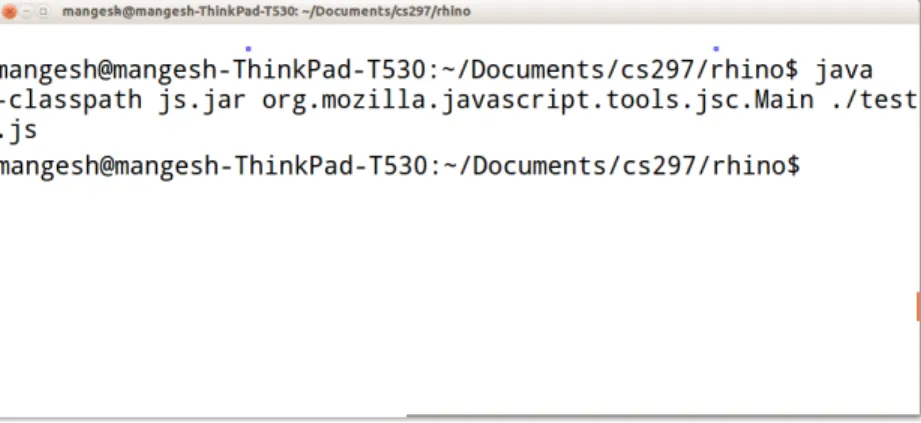
To deal with this problem, we decided to modify Rhino in such a way that it can compile JavaScript of any length and disable optimization. As we are not interested in the class file, we decided to extract opcodes at compile time. This saved the time of decompilation of class file to extract opcode sequence. This also solved the problem of optimization, as we were extracting opcodes before it creates a class file. We tapped the opcode generated by opcode generator and redirected it to the standard output stream. This will print all the generated opcodes to a screen. The generated output can be collected in a file using redirect operation in Unix. Command to run Rhino:

java -classpath <path to js.jar> org.mozilla.javascript.tools.jsc.Main <Path to JavaScript file>

Figure 3 shows standard output of Rhino after compilation. After compiling JavaScript, we will find a new class file generated in the same folder. Modified Rhino generates a class file same as the class file without modification. But in addition to the class file, a list of opcodes is also generated. This list can be observed in Figure 4. We can write this output to some file using redirect operator (>).

(36)

Figure 3: Sample Compilation Without Modification

(37)

CHAPTER 5

Statistical Malware Detection

Signature based detection method is widely used for malware detection. But metamorphic malwares can easily evade the detection by altering their internal code by using one of the techniques described in Section 2.3. Using these methods, the in-ternal structure can be changed but to retain original functionality, same instructions (instructions which are responsible for functionality) have to be used somewhere in code. This keeps the statistical distribution of instructions unique in all the morphed copies. Using these statistical properties, following malware detection techniques are designed.

5.1 Hidden Markov Model Method

Hidden Markov Model(HMM) is a pattern recognition technique which can be used to detect metamorphic malware. Recently, lot of research has been going on to enhance this technique [2, 3, 8, 30, 31]. Sridhara [26] describes a method to train HMM against opcode sequence extracted from the given malware family. This HMM model is used to score the files and classify whether a file belongs to the given malware family. If the score is greater than a predefined threshold, then it is concluded that the file belongs to a given malware family. Scores are measured in terms of Log Likelihood Per Opcode (LLPO).

5.1.1 Markov Chain

Consider a sequence of symbols. Each symbol is associated with a probability which governs the transition from one symbol to other. Transition from one symbol

(38)

Figure 5: Example of HMM

to another depends upon the probability of current symbol or in other words, not on any previous symbol in the sequence. Such sequence is called as the ‘Markov Chain’ of first order [18]. Similarly𝑛𝑡ℎ order Markov Chain is defined as a sequence of symbols in which transition from one symbol to other depends on previous 𝑛−1symbols. In Hidden Markov Model terminology, each symbol is called as State.

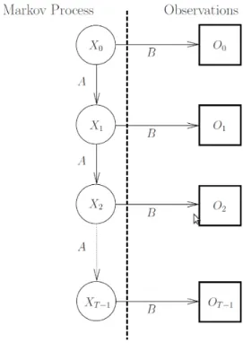
Consider an example shown in Figure 5 [2]. In this example, we have two coins one of which is biased and the other is normal. For the biased coin, probability of getting a Heads after tossing it is0.7and getting a Tails is0.3. On other hand for the normal coin, probability of getting Heads or Tails after tossing it is 0.5. We tossed a coin for 5 times which resulted in a sequence (H, T, H, H, T). H and T in this sequence represents Heads and Tails respectively. In this sequence, getting Heads or Tails depends on which coin we choose and each coin is associated with a probability of getting either a Heads or a Tails. Therefore, this sequence forms a Markov Chain. For this experiment, process of tossing coins is a Markov Process.

5.1.2 Hidden Markov Model

Hidden Markov Model(HMM) is a statistical model which represents a Markov Process whose states are unknown [27]. In [27] describes the notation used in HMM

(39)

as follows:

𝑇 = length of the observation sequence 𝑁 = number of states in the model 𝑀 = number of observation symbols

𝑄 = {𝑞0, 𝑞1, . . . , 𝑞𝑁−1}=distinct states of the Markov process

𝑉 = {0,1, . . . , 𝑀 −1}=set of possible observations 𝐴 = state transition probabilities

𝐵 = observation probability matrix 𝜋 = initial state distribution

𝑂 = (𝑜0, 𝑜1, . . . , 𝑜𝑇−1) = observation sequence.

To get a better insight about HMM, consider the same example shown in Figure 5. Here, length of the observation sequence 𝑇 is 5 as the coin is tossed for 5 times in this process. We have two different symbols in the observation sequence i.e. H and T. Therefore, value of 𝑀 for this Markov Process is 2 with 𝑉={H, T}. Transition matrix 𝐴 for this process is

A =

[︂

0.95 0.05 0.20 0.80

]︂

where, the first row represents transition probabilities for the normal coin and the second row represents transition probabilities of the biased coin. Value at position

(𝑖, 𝑗)represents transition of state from𝑖𝑡ℎ state to𝑗𝑡ℎ state. Observation probability matrix 𝐵 for this process is

A=

[︂

0.5 0.5 0.7 0.3

]︂

where, the first row represents probability of getting each observation for normal coin and the second row represents probability of getting each observation for the biased coin. Information in this matrix can be understood as—if we choose a biased coin, then probability of getting Heads is 0.7. We can pick any coin out of the given two coins. So initial state distribution will be

(40)

Figure 6: Markov Process

Matrices 𝐴, 𝐵, 𝜋 are row-stochastic which means that each row in these matrices is a probability distribution. Here, we know the values of 𝐴, 𝐵, 𝜋 and observation sequence but not the coin used for each tossing. This part of process is hidden. A model is defined using these known values as

𝜆 = (𝐴, 𝐵, 𝜋)

Figure 6 gives a graphical view of the Hidden Markov Process. The state and ob-servation of HMM at any point of time 𝑡 is represented by 𝑋𝑡 and 𝑂𝑡 respectively. Initial state 𝑋0 and matrix 𝐴 determines the hidden part of the Markov Process, as

(41)

5.1.3 HMM Implementation

Application of HMM for metamorphic malware detection is explained in greater detail in [34]. HMM model is trained using opcodes, extracted from morphed copies of malware belonging to a family. This trained model represents statistical properties of the malware family. We can compute a score for any file to determine how similar the file is to the malware family using trained HMM model. Then we can compare this score with a predetermined threshold to classify the file.

A large number of morphed versions of given malware JavaScript are generated and compiled using JavaScript compiler to obtain Java bytecode [21]. Then the opcode is extracted from these Java bytecodes. All the opcodes in training dataset are concatenated and then HMM is trained on this concatenated list of opcodes to get statistical model of the given metamorphic JavaScript malware.

To detect whether the given file belongs to the same malware family or not, we used previously generated model to calculate LLPO. If the LLPO of the program is within a particular threshold, the file is classified as a virus.

5.1.4 Log Likelihood Per Opcode

Scoring observation sequences and training the HMM involves computation of large number of products of probability distribution of opcodes. As 𝑇 increases, the resulting value of this product exponentially tends to become 0. This introduces a problem of underflow of results. To avoid this problem, forward and backward algorithms normalize the result of each iteration. This process is called scaling [27]. After application of scaling, 𝑃(𝑂|𝜆)will be calculated as

1⧸︁

𝑇−1

∏︁

𝑘=0

(42)

where𝑐𝑘 is the scaling factor at time𝑘. However, this computation is also susceptible to underflow and to avoid that, we compute Log Likelihood as

log[𝑃|𝜆] =−

𝑇−1

∑︁

𝑘=0

log𝑐𝑘

Log Likelihood is length dependent, as the sum of log transition probabilities andlog

observation probabilities will be higher for a longer sequence. As the sequence in the test set may be of different lengths compared to the sequence used to train the model, Log Likelihood will be divided by the number of opcodes in the sequence to obtain Log Likelihood per opcode which accounts for the length difference [34].

5.2 Opcode Graph Similarity

Anderson [1] describes a graph based method for malware detection. In this method, opcode sequence from given malware is extracted and a weighted directed graph is constructed using this sequence. Similar weighted graph is constructed for the file to be tested. Score for the file is calculated by taking Manhattan distance between these two graphs. Algorithm to calculate score is described in Section 5.2.2.

5.2.1 Opcode Graph

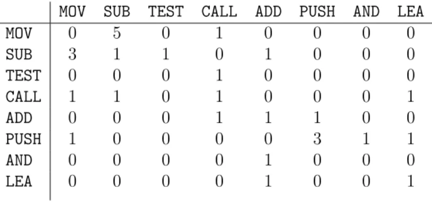
A weighted directed graph constructed from extracted opcode sequence is called as ‘Opcode Graph’. Each node of this graph is represented by a unique opcode from the opcode sequence. A directed edge is drawn from one opcode to another, if and only if, second opcode follows the first opcode in the sequence. Weight of the edge is determined by the number of occurrences of digram. Consider the opcode sequence shown in Table 1. This opcode sequence contains30opcodes. To construct a directed graph of opcodes, we need the count of digrams. In this method, we will represent this graph as an adjacency matrix as shown in Table 2.

(43)

Table 1: Opcode Sequence

Sequence No Opcode Sequence No Opcode

1 MOV 16 AND 2 SUB 17 PUSH 3 TEST 18 PUSH 4 CALL 19 MOV 5 SUB 20 CALL 6 ADD 21 CALL 7 PUSH 22 MOV 8 PUSH 23 SUB 9 AND 24 MOV 10 AND 25 SUB 11 AND 26 MOV 12 CALL 27 SUB 13 LEA 28 MOV 14 LEA 29 SUB 15 ADD 30 SUB

Table 2: Digram Count Matrix

MOV SUB TEST CALL ADD PUSH AND LEA

MOV 0 5 0 1 0 0 0 0 SUB 3 1 1 0 1 0 0 0 TEST 0 0 0 1 0 0 0 0 CALL 1 1 0 1 0 0 0 1 ADD 0 0 0 1 1 1 0 0 PUSH 1 0 0 0 0 3 1 1 AND 0 0 0 0 1 0 0 0 LEA 0 0 0 0 1 0 0 1

If you observe the row corresponding toSUBand the column corresponding toMOV, then you will get a count3for digram (SUB, MOV). If you observe opcode sequence in Table 1, you will notice that MOV instruction appeared 3 times after SUB instruction at line numbers 24, 26 and 28. Similarly, the count for each digram is tabulated in Table 2.

(44)

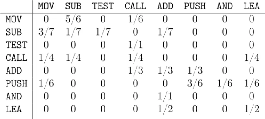
entry by the sum of that row. The resulting values will indicate the probability of occurrence of a particular opcode, after the selected opcode. For example, probability of occurrence of TEST instruction after SUB instruction will be 1 divided by 7 (sum of the entries corresponding to row SUB). After converting counts into probabilities, Table 2 will now look like Table 3.

Table 3: Digram Probability Matrix

MOV SUB TEST CALL ADD PUSH AND LEA

MOV 0 5/6 0 1/6 0 0 0 0 SUB 3/7 1/7 1/7 0 1/7 0 0 0 TEST 0 0 0 1/1 0 0 0 0 CALL 1/4 1/4 0 1/4 0 0 0 1/4 ADD 0 0 0 1/3 1/3 1/3 0 0 PUSH 1/6 0 0 0 0 3/6 1/6 1/6 AND 0 0 0 0 1/1 0 0 0 LEA 0 0 0 0 1/2 0 0 1/2 5.2.2 Similarity Calculation

Probability matrices for files to be compared are created by the procedure de-scribed above. Similarity between two files is calculated by taking the Manhattan distance between two probability matrices. Suppose 𝐴 is the probability matrix for file 1 and each element in 𝐴 is represented as 𝑎𝑖,𝑗 where 𝑖 and 𝑗 represents 𝑖𝑡ℎ row and 𝑗𝑡ℎ _{column. Similarly for file 2,} _𝐵 _{is the probability matrix and each element is} represented as 𝑏𝑖,𝑗. Similarity is calculated by

score = 1 𝑁2 (︃_𝑁₋₁ ∑︁ 𝑖,𝑗=0 |𝑎𝑖,𝑗−𝑏𝑖,𝑗|2 )︃

(45)

5.2.3 Implementation

To use this similarity score for metamorphic malware detection, we need to set a suitable threshold. To set the threshold value, we followed the steps below:

1. Calculate opcode graph for known metamorphic malware samples. 2. Calculate opcode graph for morphed versions of malware samples. 3. Calculate opcode graph for benign files.

4. Calculate score for morphed versions vs known metamorphic malware samples. 5. Calculate score for benign files vs known metamorphic malware samples. 6. Set threshold based on step 4 and step 5.

For our implementation, we chose the highest score from step 4 and the lowest score from step 5. Average of these two values is considered as the threshold. If score of any file is less than this threshold, it is classified as a malware.

5.3 Simple Substitution Distance

Simple Substitution Distance method is a hill climbing technique based on Jakob-sen’s algorithm for simple substitution cryptanalysis [13]. In this method, it is as-sumed that frequency order of opcodes hold true to a certain extent for every malware family. This allows us to calculate similarity between any two files using Jakobsen’s algorithm. In Jakobsen’s algorithm, the score gives the degree to which the putative plaintext matches the plaintext language statistics. The score given by Simple Sub-stitution Distance method can be viewed as a measure of the distance between the opcode sequence of a given file and the opcode statistics of a metamorphic family [23].

(46)

5.3.1 Jakobsen Algorithm

Basic assumption in Jakobsen’s algorithm is that the plain text is in English language and Ciphertext contains 26 different symbols. Each symbol maps to one of the 26 different letters in English. Algorithm starts with calculating the frequency of the symbols in the ciphertext and arranging them in the decreasing order of their occurrence frequency. Putative key is then calculated by mapping these symbols from the ciphertext to the letters in English arranged in the standard frequency order. This key is altered in each iteration after looking at the obtained plain text. Suppose key ‘K’ is initial key, then it can be represented as

K = 𝑘1, 𝑘2, 𝑘3, . . . , 𝑘26

where each 𝑘𝑛 is mapping of one symbol from cipher text on some English letter. In each iteration algorithm modifies key ‘K’ slightly. This new key is used to decrypt ciphertext and then the newly generated putative plain text is checked. If putative plain text is closer to the original plain text, then the change in key is retained and algorithm starts again considering the obtained modified key as the putative key. A scheme is followed to modify the key. Initially, symbols adjacent to each other are swapped and cipher text is decrypted to check correctness of the key. Suppose, we have the putative key as shown above, then initially swapping is done in 𝑘1 and

𝑘2. In next iteration, swapping will be done in 𝑘2 and 𝑘3 and so on. This can be

viewed as first round of swapping in which we swap adjacent element. In next round, elements at places 𝑖𝑡ℎ _and ₍_𝑖_{+ 2)}𝑡ℎ _{are swapped. In the successive rounds, distance} between to be swapped elements is increased by 1. In all, there can be (︀26₂)︀ different

(47)

ways in which the key can be altered. This scheme of swapping can be visualized as round 1: 𝑘1|𝑘2 𝑘2|𝑘3 𝑘3|𝑘4 . . . 𝑘23|𝑘24 𝑘24|𝑘25 𝑘25|𝑘26 round 2: 𝑘1|𝑘3 𝑘2|𝑘4 𝑘3|𝑘5 . . . 𝑘23|𝑘25 𝑘24|𝑘26 round 3: 𝑘1|𝑘4 𝑘2|𝑘5 𝑘3|𝑘6 . . . 𝑘23|𝑘26 .. . ... . .. round 24: 𝑘1|𝑘24 𝑘2|𝑘25 𝑘3|𝑘26 round 25: 𝑘1|𝑘25 𝑘2|𝑘26 round 26: 𝑘1|𝑘26

To test the correctness of the key, algorithm creates a digram matrix of English letters from plain text. Each entry in matrix represents frequency count of that digram in plain text. This matrix is referred as 𝐸 matrix in the algorithm. Similarly, another digram matrix is created from decrypted text. This matrix is called as 𝐷 matrix in the algorithm. Correctness of the key is calculated as

score (k)=∑︁

𝑖,𝑗

|𝑑𝑖,𝑗−𝑒𝑖,𝑗|

where, 𝑑𝑖,𝑗 and 𝑒𝑖,𝑗 refers to 𝑖𝑡ℎ and 𝑗𝑡ℎ element in 𝐷 and 𝐸 matrices respectively. In each iteration of the algorithm, the score is calculated. If the score is smaller than the score obtained in previous iteration, it is retained else discarded. In other words, lower the score, better is the decrypted text. At the end of the algorithm, if the obtained decrypted text is the same as the original text, then the score will become zero. As a result, we will get the key and decrypted text, which will be similar to the original plain text.

In this method, we extracted the opcode sequence from generated morphed ver-sions of the given malware JavaScript. Then the frequency of each opcode is counted. All opcodes are arranged in the decreasing order of their count. Consider we get the

(48)

opcode order as

MOV,ADD,LOAD,SUB,JMP,CMP

This will be called as standard opcode order for the given malware. Then digram frequency graph is constructed by using the same opcode sequence. In this graph, each entry will represent frequency count of a digram. Adjacency matrix is used to represent this graph. This adjacency matrix will be analogous to 𝐸 matrix in Jakobsen’s algorithm [13]. The opcode sequence is then extracted from the file to be tested. Frequency of each opcode is counted and arranged in decreasing order of their frequency count. Suppose we get the opcode sequence as

ADD,SUB,CMP,LOAD,MOV,MUL,JMP

This opcode order is mapped to previously calculated standard opcode order. This mapping will give us the putative key. Initial putative key is shown in Table 4. After

Table 4: Opcode Mapping (Putative Key)

Standard Opcode Order MOV ADD LOAD SUB JMP CMP OTHER

Test Opcode Order ADD SUB CMP LOAD MOV MUL JMP

doing one to one mapping, if testing file contains more unique opcodes, then they will be mapped to dummy opcodeOTHER. Then all opcodes in testing file are replaced with corresponding opcode in the putative key. A digram matrix is created from the replaced opcode sequence. This matrix is analogous to 𝐷 matrix in Jakobsen’s algorithm. A score is calculated by taking Manhattan distance between the𝐷and 𝐸 matrices.

score=∑︁

𝑖,𝑗

|𝑑𝑖,𝑗 −𝑒𝑖,𝑗|

Key swapping is then done in the putative key by swapping the adjacent elements. For example, we have the putative key as shown in Table 5. First swapping occurs

(49)

between ADDand SUB to give a new putative key as shown in Table 6. Table 5: Key Before Swapping

Test Opcode Order ADD SUB CMP LOAD MOV MUL JMP

Table 6: Key After Swapping

Test Opcode Order SUB ADD CMP LOAD MOV MUL JMP

By using this new key, we calculate scores for the given test file again. To reflect the changes made in the key, we need to construct a new𝐷matrix. The new𝐷matrix will be constructed by swapping the rows and columns in the previously constructed 𝐷 matrix. Suppose we have a 𝐷 matrix as shown in the Table 7.

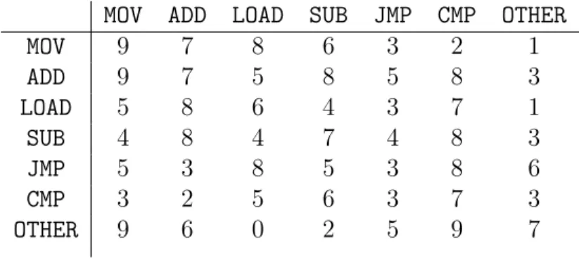
Table 7: D Matrix before Swapping

MOV ADD LOAD SUB JMP CMP OTHER

MOV 9 7 8 6 3 2 1 ADD 9 7 5 8 5 8 3 LOAD 5 8 6 4 3 7 1 SUB 4 8 4 7 4 8 3 JMP 5 3 8 5 3 8 6 CMP 3 2 5 6 3 7 3 OTHER 9 6 0 2 5 9 7

As we swap entries corresponding toMOVand ADDin the putative key, to achieve the same effect on 𝐷 matrix, we need to swap the rows and columns corresponding toMOV and ADD. After swapping, we will get a new 𝐷 matrix as shown in Table 8.

Thereafter, score is calculated by taking the Manhattan distance between the newly created 𝐷 matrix and 𝐸 matrix. If the new score is greater than the previous score, then we discard the swapping and move towards next swapping. Here in this

(50)

Table 8: D Matrix after Swapping

MOV ADD LOAD SUB JMP CMP OTHER

MOV 7 9 5 8 5 8 3 ADD 7 9 8 6 3 2 1 LOAD 8 5 6 4 3 7 1 SUB 8 4 4 7 4 8 3 JMP 3 5 8 5 3 8 6 CMP 2 3 5 6 3 7 3 OTHER 6 9 0 2 5 9 7

example, next swapping will be done between MOVand LOAD. If the new score is less than the previously calculated score, then we will retain the swapping and continue algorithm from beginning, keeping swapped key as the putative key.

In the first round, swapping will be done between adjacent elements in the key. In next round, swapping will be done between elements on the𝑖𝑡ℎ_and _𝑖_{+ 2}𝑡ℎ _position in the key. In successive rounds, distance between elements to be swapped is increased by one. This swapping scheme can be visualized as

round 1: 𝑘1|𝑘2 𝑘2|𝑘3 𝑘3|𝑘4 . . . 𝑘𝑛−3|𝑘𝑛−2 𝑘𝑛−2|𝑘𝑛−1 𝑘𝑛−1|𝑘𝑛 round 2: 𝑘1|𝑘3 𝑘2|𝑘4 𝑘3|𝑘5 . . . 𝑘𝑛−3|𝑘𝑛−2 𝑘𝑛−2|𝑘𝑛 round 3: 𝑘1|𝑘4 𝑘2|𝑘5 𝑘3|𝑘6 . . . 𝑘𝑛−3|𝑘𝑛 .. . ... . .. round n-2: 𝑘1|𝑘𝑛−2 𝑘2|𝑘𝑛−1 𝑘3|𝑘𝑛 round n-1: 𝑘1|𝑘𝑛−1 𝑘2|𝑘𝑛 round n: 𝑘1|𝑘𝑛

The smallest score achieved in this process is the score of similarity. To classify a file, this score is compared against a predefined threshold. If the score is less than the threshold value, then file under consideration belongs to the given malware family.

(51)

5.4 Singular Value Decomposition

Singular Value Decomposition is a technique used in image detection which can also be used to detect malware files. Deshpande [9] describes a method based on Singular Value Decomposition to detect metamorphic malware. The scores are cal-culated by taking euclidean distance between weights of known malware sample and unknown malware sample. Weights are calculated by projecting column vector of a file on a space enclosed by eigenvectors of a known malware [14]. This enclosed space is called as eigenspace.

Eigenspace is calculated by projecting eigenvectors of covariance matrix. Covari-ance matrix is calculated as 𝐴𝐴𝑇_{. Singular Value Decomposition of a matrix} _𝐴 _is represented as

𝐴=𝑈 𝑆𝑉𝑇

where,𝑈 is covariance matrix. 𝑆 is a diagonal matrix with square root of eigenvalues common to both matrices𝑈 and 𝑉.

5.4.1 Algorithm

The algorithm works in two phases—Training Phase and Testing Phase. In Training Phase, weights of known malware files are calculated by projecting them on to the eigenspace. In Testing Phase, we project files to be tested on to the same eigenspace and calculate their corresponding weights. Thereafter, euclidean distance between previously calculated and newly calculated weights are taken to compare them against the threshold value. Following sections will describe these two phases stepwise.

(52)

5.4.1.1 Training Phase

∙ In training phase, raw bytes from text or code section of training dataset are extracted. These raw bytes are converted into decimal values to construct a column vector.

∙ Then covariance matrix is constructed. Covariance matrix is a product of ma-trix 𝐴 and its transpose. Matrix 𝐴 is constructed by appending all column vectors. Suppose we have𝜑1, 𝜑2, 𝜑3, . . . , 𝜑𝑀 column vectors, then matrix A can be constructed as

𝐴= [𝜑1 𝜑2 𝜑3 . . . 𝜑𝑀]

∙ Now, Eigenvectors for covariance matrix are calculated. These eigenvectors determine eigenspace. Eigenvectors with large eigenvalues represents prominent characteristics of a malware. So, we ignore eigenvectors with small eigenvalues.

∙ All eigenvectors are arranged in the descending order of their eigenvalues. For our experiment, we consider top M’ eigen vectors from M eigenvectors (where M’ < M). We project these eigenvectors onto the space. Space bounded by these eigenvectors is called eigenspace.

∙ Original malware can be constructed by using these M’ eigenvectors by adding them with their weights. Suppose for a malware 𝑉 we have 𝑒1, 𝑒2, 𝑒3, . . . , 𝑒𝑀′ eigenvectors with corresponding weights 𝑤1, 𝑤2, 𝑤3, . . . , 𝑤𝑀′. Then malware 𝑉 can be reconstructed as 𝑉 =𝑒1×𝑤1 +𝑒2×𝑤2+. . .+𝑒𝑀′ ×𝑤_𝑀′ 𝑉 = 𝑀′ ∑︁ 𝑖=1 𝑤𝑖 ×𝑒𝑖

(53)

Therefore, weights for each sample can be obtained by 𝑤𝑖 = 𝑀′ ∑︁ 𝑖=0 𝑒𝑇_𝑖 ×𝑉

The obtained weights for a particular virus 𝑉𝑖 can be represented as

Ω𝑇_𝑖 = [𝑤𝑖, 𝑤2, 𝑤3, . . . , 𝑤𝑀′]

∙ Obtained weights for all malware samples can be represented as ∆ ∆ = [Ω1,Ω2,Ω3, . . . ,Ω𝑀]

5.4.1.2 Testing Phase

∙ In this phase, we first construct a column vector for each file which is to be tested. If the size of the file is less than𝑁 bytes, then column vector is appended with zeros. And if size of the file is more than 𝑁 bytes, then column vector is constructed by taking first𝑁 bytes from file.

∙ This column vector is projected on to the previously calculated eigenspace. Weights for file T which is to be tested can be calculated by

𝜔𝑖 = 𝑀′ ∑︁ 𝑖=0 𝑒𝑇_𝑖 ×𝑉𝑛 Ω𝑇_𝑛 = [𝜔1, 𝜔2, 𝜔3, . . . , 𝜔𝑀′]

∙ Euclidean distance between Ω𝑛 vector and weight vector generated in training phase can be calculated by

Distance= √︁ (𝜔2 1 −𝑤12) + (𝜔22−𝑤22) +. . .+ (𝜔𝑀 ′ 1 −𝑤𝑀 ′ 1 )

where,𝜔 represents weight of test file and 𝑤 represents weight of training file.

∙ A threshold is calculated by testing few known malware files which belong to the same malware family.

(54)

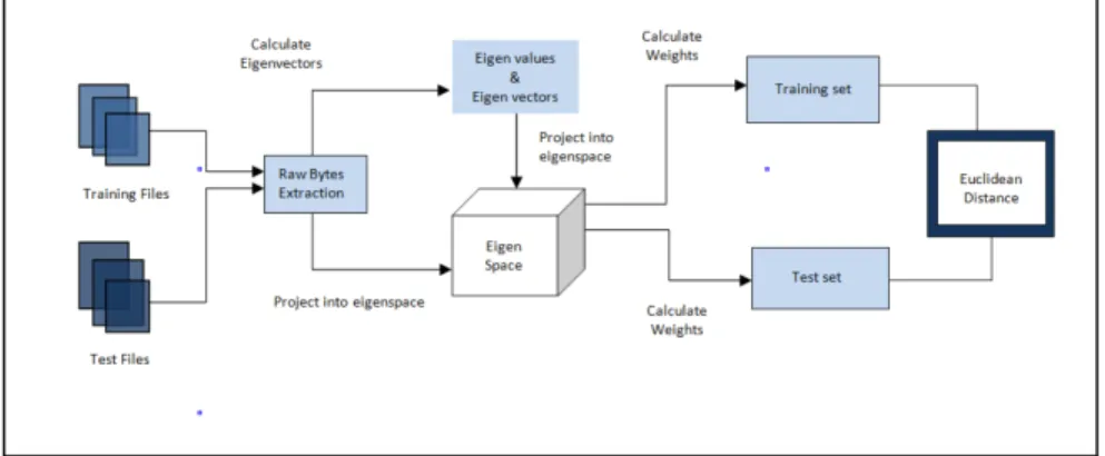
Figure 7: SVD Process

To implement above described algorithm to detect given JavaScript malware family, we compiled JavaScript into Java byte code. To every byte code, there is an equivalent hex value associated. We converted those hex values to decimal values. Suppose we have 𝑀 files in the training dataset, each file having different number of bytes. The largest file has 𝑁 bytes, using which an 𝑁 ×𝑀 matrix is created. Zeros are appended to smaller files and first𝑁 bytes are chopped from the larger files. This matrix is called a covariance matrix.

We pass this matrix to JAMA API which is developed in Java to calculate eigen-vectors and eigenvalues. These obtained eigeneigen-vectors form a eigenspace which is used to calculate the weights. Weights for files which we want to test are calculated by projecting their column vectors on the generated eigenspace. This whole process can be visualized as shown in Figure 7. Once we get the weights for both the training set and the files to be tested, then scores are calculated by taking the euclidean distance between weights of the training files and the testing files. Experimental analysis of given JavaScript malware is explained in Section 6.

(55)

CHAPTER 6 Experiments

This chapter discusses about the experimental setup, files used in the experiment and results obtained from these experiments. Experiment involves implementation and testing of the following methods:

∙ Hidden Markov Model Method

∙ Opcode Graph Similarity Method

∙ Simple Substitution Distance Method

∙ Singular Value Decomposition Method

All these methods work on statistical properties of opcodes. Given malware files are written in JavaScript. To convert JavaScript code into opcode sequence, we used the Rhino JavaScript Engine. We modified Rhino in such a way that it gives opcode sequence at compile time as discussed in Section 4. We performed all these experiments on a machine with the following configuration.

Table 9: Machine Specifications

Model Lenovo ThinkPad T530

Processor 3rd Generation Intel Core i7-3110M @2.80GHz

RAM 8.00GB

System type 64-bit OS

Java Compiler Java 6

Operating System Ubuntu 12.10

The given JavaScript malware carries a morphing engine with itself. After every infection, the internal structure of malware gets changed. For the experiments, we

(56)

generated 100 morphed versions of the given malware. These files are used in training phase and testing phase.

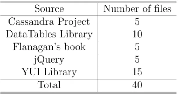
The experiments undertaken need benign files to test the proposed detection method. We collected benign files from different open source JavaScript libraries [5, 7, 12, 15, 36]. Effectiveness of each method is judged by plotting Receiver Operating Characteristics (ROC) curve [4]. Area under the ROC curve will give us the degree of correctness for every individual method.

Table 10: Source of Benign Files Source Number of files

Cassandra Project 5 DataTables Library 10 Flanagan’s book 5 jQuery 5 YUI Library 15 Total 40

6.1 Receiver Operating Characteristics

Receiver Operating Characteristics (ROC) curve is a graphical representation for correctness of classification system [4]. It is created by plotting true positives out of the total actual positives (called as TPR = true positive rate) vs. the fraction of false positives out of the total actual negatives (called as FPR = false positive rate), at various threshold values. TPR and FPR are also known as sensitivity and fall out of classification system. For plotting ROC curve, we first calculate probabilities for true positive and false positive. Then a curve is generated by plotting the cumulative distribution function of the true positive probabilities on the y-axis vs the cumulative distribution function of false positive probabilities on the x-axis [11]. The Area Under the Curve (AUC) of ROC gives a measure of correctness of classification. Following

(57)

Figure 8: HMM Score Analysis (N=2)

sections will discuss results of above mentioned method by plotting ROC curves for each method.

6.2 Hidden Markov Model

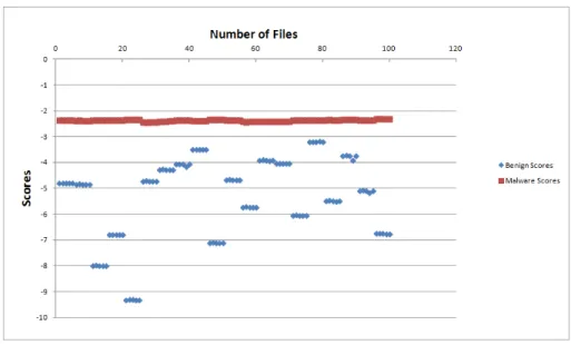
To test the correctness of HMM method, we did a number of experiments. It has been observed that number of states do not make any significant difference in the score calculation. So, we decided to continue with number of states equal to 2. Opcode sequence for benign files and malware files are same as discussed above. We randomly choose 20 opcode sequences from generated pool of malware samples to train HMM. Then we calculated scores for rest of the malware samples and benign files. To visualize the distribution of scores we plotted Scatter plot for the obtained scores. Scatter Plot shown in Figure 8 clearly depicts the distinction between score of malware and benign files.

The effectiveness of HMM can be judged using the ROC curve [4]. ROC curve for the above described experiment is shown in Figure 9. As area under the curve

(58)

Figure 9: ROC curve for HMM

(AUC) is 1, it shows that trained HMM model is correctly distinguishing between virus files and benign files.

6.3 Opcode Graph Similarity Method

For this experiment, we used same malware files and benign files as discussed above. Threshold is determined by the method described in Section 5.2.3. Purpose of this experiment is to verify whether the computed scores for benign files and malware files are distinguishable or not.

Scores are obtained in this experiment are plotted on scatter graph as shown in Figure 10. Red points in graph shows scores of malware file vs malware file and green points shows scores of malware file vs benign file. It can be observed from Table 10 that scores for malware file vs malware file are in order of10−2 _{while scores}

for malware file vs benign file are in order of10−1_{. From this, we can clearly conclude}

that this method is distinguishing files correctly.

ROC curve for the experiment is shown in Figure 11. Area under the curve is 1, which shows perfect classification between malware files and benign files.

(59)

Figure 10: Opcode Graph Similarity Analysis

Figure 11: ROC curve for Opcode Graph Similarity Method

6.4 Simple Substitution Distance Method

For this experiment, we have randomly selected 10 virus files from a pool of generated morphed copies of malware and 10 benign files. Their scores are listed below in Table 11. Looking at the score in Table 11, we can conclude that distribution of opcode frequency in malware samples is consistent. On the other hand, as the score for the benign file is large, it shows that the distribution of opcode frequency differs

(60)

Figure 12: Simple Substitution Method Scores Analysis

a lot.

Table 11: Simple Substitution Method Scores File name Score File Name Score

Ben_1 2.65007 Virus_1 1.82535 Ben_2 2.52474 Virus_2 1.82537 Ben_3 2.49072 Virus_3 1.82537 Ben_4 2.58470 Virus_4 1.82537 Ben_5 2.65446 Virus_5 1.82539 Ben_6 2.66617 Virus_6 1.82539 Ben_7 2.64091 Virus_7 1.82537 Ben_8 2.65737 Virus_8 1.82537 Ben_9 2.66809 Virus_9 1.82539 Ben_10 2.64965 Virus_10 1.82537

Scatter Plot in Figure 12 clearly shows the distinction between scores of malware and benign files. For the same experiment, we have drawn a ROC curve as shown in Figure 13. Area under the curve is 1, which indicates perfect classification of files.

(61)

Figure 13: ROC for Simple Substitution Method

6.5 Singular Value Decomposition Method

We randomly selected 20 samples of benign JavaScript and malware JavaScript files from above mentioned pool of benign files and malware samples. Opcodes from these files are then converted to decimal equivalent with the help of opcodes to hex value mapping. Eigenspace is created using training malware samples. Weights of files (files to be tested) are obtained by projecting their column vectors on previously generated eigenspace. Scatter plot of these values is shown in Figure 14.

To test the effectiveness of experiment, we plot ROC curve for the scores obtained in experiment. The ROC curve for the experiment is as shown in Figure 15. Area under the Curve is 1. AUC 1 shows that algorithm described in Section 5.4 perfectly distinguish between malware samples and benign samples.

(62)

Figure 14: SVD Scatter Plot Analysis

(63)

CHAPTER 7 Enhancement

Looking at the analysis of given malware using Hidden Markov Model, Simple Substitution Method, Opcode Graph Similarity method and Singular Value Decom-position method, it is clear that given malware can be detected by methods based on statistical properties of opcodes. To evade such detection we executed an experiment by inserting deadcode into given JavaScript malware.

To implement this, we have created a service which will run on central server. Whenever malware gets executed, it creates a connection with this central server. A random number n is passed to the service. This service will generate n number of functions and send back to malware. The malware then adds this deadcode to its body. By adding this deadcode, functionality will remain same but the statistical characteristic of opcode sequence will change. This will help to evade detection by above mentioned methods.

7.1 Hidden Markov Model

To evade the detection by Hidden Markov Model we modified the service which will insert deadcode in controlled amount. We chose 20 morphed versions of the given malware. Then we created different versions of chosen files by adding deadcode. Initially we started with 100 random functions as deadcode. Then we compiled this new version with the help of Rhino and got opcode sequence for chosen files. Scores are calculated against previously calculated models.