A Nonparametric Statistical Comparison of Principal Component and Linear
Discriminant Subspaces for Face Recognition
J. Ross Beveridge, Kai She and Bruce A. Draper
Geof H. Givens
Computer Science Department
Statistics Department
Colorado State University
Colorado State University
Fort Collins, CO, 80523
Fort Collins, CO, 80523
Abstract
The FERET evaluation compared recognition rates for different semi-automated and automated face recognition algorithms. We extend FERET by considering when differ-ences in recognition rates are statistically distinguishable subject to changes in test imagery. Nearest Neighbor clas-sifiers using principal component and linear discriminant subspaces are compared using different choices of distance metric. Probability distributions for algoriithm recognition rates and pairwise differences in recognition rates are de-termined using a permutation methodology. The principal component subspace with Mahalanobis distance is the best combination; using L2 is second best. Choice of distance measure for the linear discriminant subspace matters little, and performance is always worse than the principal com-ponents classifier using either Mahalanobis or L1 distance. We make the source code for the algorithms, scoring proce-dures and Monte Carlo study available in the hopes others will extend this comparison to newer algorithms.
1. Introduction
The FERET evaluation [12] established a common data set and a common testing protocol for evaluating semi-automated and semi-automated face recognition algorithms. It illustrated how much can be accomplished in a well coordi-nated comparative evaluation. That said, the FERET eval-uation stopped short of addressing the critical question of statistical variability. In short, which of the measured dif-ferences in algorithm performance were statistically distin-guishable, and which essentially matters of chance.
Answering this question is not a simple matter, for it begs other questions such as what is the larger population under consideration and what are the intrinsic sources of uncertainty in the testing procedure. In their broad form, these question go far beyond the scope of any single
pa-per, including this one. Here we will consider whether the observed difference in percentage of people correctly rec-ognized using different algorithms exceeds what might be expected by chance alone, if the target population is limited to the sample.
Seven algorithm variants are considered. Four are near-est neighbor classifiers using a subspace defined by princi-pal components derived from training imagery. Three use the principal components to reduce image dimensionality and then perform nearest neighbor classification in a further subspace defined by linear discriminants. The linear dis-criminants are derived from class labeled training imagery. The four principal component analysis (PCA) algorithms use L1, L2, angle and Mahalanobis distance respectively in the nearest neighbor phase. The three linear discrimi-nant analysis (LDA) algorithms use L1, L2 and angular dis-tance respectively. The percentage of people recognized, or recognition rate, is used to compare algorithm performance. Recognition rate may be parameterized at different ranks, where rank1means the nearest neighbor is an image of the same person, and rankkmeans an image of the same person is among the topknearest neighbors.
A Monte Carlo sampling procedure is used to estimate the recognition rate distribution for each algorithm under the assumption that each person’s gallery images are ex-changeable, as are each person’s probe images. Keeping with common FERET terminology, gallery images are ex-emplars of the people already known to the system and probe images are novel images to be recognized. The test-ing data used in this study consists of4images for each of 160distinct individuals. Initially, we endeavored to design a bootstrapping [5] study, but difficulties described below led us to instead favor permuting probe and gallery choices. Permuting the images selected to serve as gallery and probe generates sample gallery and probe sets that always contain one instance of each person.
We write this paper for two reasons. First, while neither of the algorithms being tested are by any means state-of-the-art, they are both fundamental and well known. Each
repre-sents, in a pure form, the expression of a mature branch of pattern classification. Second, there is nothing in our Monte Carlo methodology that is particular to the algorithms stud-ied here. Our algorithms, scoring and statistical evaluation code are available through our web site1and we hope others will use them to establish baselines against which to assess the performance of new algorithms.
1.1. Previous Work
The FERET evaluation [12] provided a large set of hu-man face data and established a well defined protocol for comparing algorithms. The FERET data is now available to research labs working on face recognition problems [6]. The primary tool used to compare algorithm performance in FERET was the Cumulative Match Score (CMS) curve. Recognition rate for different algorithms is plotted as a function of rankk. Curves higher in the plot represent al-gorithms doing better. This same comparison techniques is used in the more recent Facial Recognition Vendor Test 2000 [3].
The FERET evaluation did not establish a common means of testing when the difference between two curves was significant. At the end of the FERET evaluation, a large probe set was partitioned into a series of smaller probe sets, and algorithms were ranked based upon performance on each partition. Variation in these rankings suggested how robust an algorithm’s position in the ranking was relative to changes in test data ([12] Tables 4 and 5). This represents a first attempt to address the issue of variation associated with changes in the test data.
As a baseline algorithm, FERET used an Eigenface algo-rithm that represented the line of classification algoalgo-rithms based upon PCA that arose from the work by [11, 10]. The PCA algorithm used here is for all intents and pur-poses equivalent to the Eigenface algorithm used in FERET. One of the top performing algorithms in the FERET evalu-ation was an LDA algorithm developed by Zhao and Chel-lapa [17]. Of the top performing algorithms in FERET, this is the one based upon the oldest and best understood sub-space projection technique after PCA [4, 1]. For both these reasons, a similar LDA algorithm has been chosen for our study.
Stepping back from face recognition, characterizing the performance of computer vision algorithms has been an on-going concern [7, 9] and more is certainly being done in this area each year. In comparison, however, far more is written each year about new and different algorithms. See [14, 15] for recent surveys of face recognition algorithms. Thus, while the literature on algorithms is vast, little has been written about using modern statistical methods [2] to mea-sure uncertainty in performance meamea-sures.
1http://www.cs.colostate.edu/evalfacerec/
One notable exception is the work by Micheals and Boult [13]. Micheals and Boult use a statistical technique to derive mean and standard deviation estimates for recog-nition rates at different ranks. They compare a standard PCA algorithm to two algorithms from the Visionics’ FaceIt SDK on essentially the same set of FERET data as we con-sider here. Using a techniques called balanced replicate re-sampling, they develop standard error bars for CMS curves. Their conceptual development is quite different from ours, but we employ quite similar resampling steps. One differ-ence in emphasis is that Micheals and Boult pair their re-sampling with analytic results to derive estimators of means and variances. In contrast, here we will present the ac-tual distributions and illustrate how to make statistical in-ference directly from the resampling results. This will en-able a direct examination of hypotheses such as algorithm A is better than algorithm B. There is an ongoing collabora-tion between us and these authors, and we anticipate future work showing more clearly the relationships between our approaches.
2. Recognition Algorithms
2.1. PCA Algorithm
While the standard PCA algorithm is well known, we include a brief description in order to be completely clear as to how our particular variant is constructed. The PCA subspace is defined by a scatter matrix formed by training images. A set ofmtraining imagesT may be viewed as a set of column vectors containing the images expressed as vectors containingnpixel valuesv
x;y: T =fx 1 ;x 2 ;:::;x M g x i = v 1;1 ::: v r;c T (1) Equivalently, the mimages may now be viewed as points in<
n
. The centroid of the training imagesx
is subtracted from each image when forming thenbymdata matrixX.
X = x 1 x ::: x P x ; x = 1 P P X i=1 x i (2) The scatter matrixis now defined to be
=XX T
(3) When properly normalized,is a sample covariance ma-trix. The Principal Components are the eigenvectors of. Thus
E=E (4)
defines the PCA basis vectors,E, and the associated eigen-values . It is common to sortE by order of decreasing eigenvalue and to then truncateE, including only the most
significant principal components. The result is ann byd orthogonal projection matrixE
d.
The PCA recognition algorithm is a nearest neighbor classifier operating in the PCA subspace. The projection y
0
of an imageyin PCA subspace is defined as
y 0 =E d (y x ) (5) During training,E dand x
are constructed and saved. Dur-ing testDur-ing, exemplar images of the people to be recognized are projected into the PCA subspace. A novel image is rec-ognized by first being projected into PCA subspace and then compared to exemplar images already stored in the sub-space.
2.2. Distance Measures
Four commonly used distance measures are tested here: L1 , L2, angle and Mahalanobis distance, where angle and Mahalanobis distance are defined as:
Angle Negative Angle Between Image Vectors
Æ(x;y )= xy kxkky k = P k i=1 x i y i q P k i=1 (x i ) 2 P k i=1 (y i ) 2 (6)
Mahalanobis Mahalanobis Distance
Æ(x;y )= k X i=1 1 p i x i y i (7) Where iis the
ith Eigenvalue corresponding to theith Eigenvector.
2.3. PCA plus LDA Algorithm
The LDA algorithm uses the PCA subspace projection as a first step in processing the image data. Thus, the Fisher Linear Discriminants are defined in theddimensional sub-space defined by the firstdprincipal components. This de-sign choice is consistent with prior uses of LDA algorithms to perform face recognition [17].
Fisher’s method definesc 1basis vectors wherecis the number of classes. These basis vectors may be expressed as rows in a matrixW, and the discriminants are defined as those basis vectors that maximize the ratio of distances between classes divided by distances within each class:
J(W)= WM B W T WM W T (8) where M W = c X i=1 M i ; M i = n i X j=1 (y j i )(y j i ) T (9) and M B = C X i=1 n i ( i )( i ) T (10) The basis vectors are the row vectors inW that maximize J(W). Text books often state thatW is found by solving the general eigenvector problem [4]:
M B
W =M W
W (11)
This is true, but provides no insight into why. Nor is it al-ways the best way solve forW [18]. We have written a report [8] illustrating the underlying geometry at work and filling out the solution method used in [18].
Projecting an imageyinto LDA subspace yieldsy 00 : y 00 =Wy 0 =WE d (y x ) (12)
Training images must be partitioned into classes, one class per person. They are used to determine E
p, x
and W. During testing, the LDA algorithm performs classification in LDA space in exactly the same manner that the PCA al-gorithm performs classification in the PCA subspace.
3. Research Question
The complete FERET database includes14;051source images, but only 3;819show the subjects directly facing the camera. Of these, there are 1;201distinct individuals represented. For481of these people, there are3or more images, and for256there are4or more images. Being more precise, of the256people with four or more images, there are160where the first pair was taken on a single day, and the second pair on a different day. Of the images taken on the same day, the subject was instructed to pick one facial expression for the first image and another for the second 2
In our study, algorithms will be trained using 675 im-ages of225people for whom there are three, but not four images. Algorithms will be tested on the640images of the 160people with pairs of images taken on different days. The question of interest is:
How much variation in recognition rate can be ex-pected when comparing gallery images of these individuals taken on one day to probe images taken on another day?
2It might surprise some readers to note that no further instruction was given. Specifically the subjects were not coached as to what sort of expres-sion to adopt, for example smile of frown, happy or sad. So, it is incorrect to assume anything other than that the expressions are different.
Clearly this is not the only question we might pose. How-ever, it is an important question and sufficient to illustrate our method.
4. Preprocessing and Training
Both algorithms considered here are semi-automated in that they require the face data be spatially normalized. In addition, both algorithms required training. Both proce-dures are explained below.
4.1. Image Preprocessing
All our FERET imagery has been preprocessed using code originally developed at NIST and used in the FERET evaluations. We have taken this code and converted it to straight C, instead of C++, and we have separated it from the large set of NIST libraries that come with the FERET data distribution. Thus, it is one source file that compiles by itself and is available through our web site.
Spatial normalization rotates, translates and scales the images so that the eyes are placed at fixed points in the im-agery based upon a ground truth file of eye coordinates sup-plied with the FERET data. The images are cropped to a standard size,150by130pixels. The NIST code also masks out pixels not lying within an oval shaped face region and scales the pixel data range of each image within the face re-gion. In the source imagery, grey level values are integers in the range0to255. These pixel values are first histogram equalized and then shifted and scaled such that the mean value of all pixels in the face region is zero and the standard deviation is one.
4.2. Algorithm Training
For the tests presented here, we choose to focus on is-sues relating solely to changes in the test data and not to consider the broader question of uncertainty introduced by changes in training data. This is to not suggest that vari-ation due to training is unimportant. However, the Monte Carlo method used here must sample from the space of ex-periments thousands of times. Were such sampling done by brute force retraining on each sample, the computational burden would be staggering. In the past we have studied variation in both PCA and LDA performance subject to re-training [16]. In future we will investigate ways to adapt our methodology efficiently to questions involving changes to the training data.
Since it is desirable to have no overlap between training and test data, and since the data with4images per person is highly valuable for testing, it was decided to use the im-agery of the225people for whom there are at least three, but not four, images each for training. Consequently, the
PCA algorithm was trained using675images. In keeping with common practice in the FERET evaluation, the top40 percent of the eigenvectors were retained. The LDA algo-rithm was trained on the same images partitioned into225 classes, one class per person.
Readers very familiar with how these subspace projec-tion algorithms operate may already have determined the dimensionality of the subspaces implied by the above state-ments. For the rest, here is the summary. The projection from image space to PCA space maps from<
19;500 to<
270 : 270is40percent of675. The projection from PCA space to LDA space is a projection from<
270 to<
224 .
There are relatively few other choices to make in setting up these two algorithms. One is the distance metric, and we consider several common alternatives. Additionally, for the LDA algorithm the nature of the training data is criti-cal. While the decision to use the675images,3images per person, is the obvious one given our data constraints, it is far from ideal. On the order of10or100images per per-son would be a much better number for training. Also, it is an open question whether having so many people,225, and thus such a high dimensional LDA subspace, is good. Past LDA work has used fewer individuals, and some have used a synthetic alteration processes to boost the training images per class [17]
5. Data Setup and Recognition Rate
Day 1 Day 2
Expression Expression Person One Another One Another
0 I 0;0 I 0;1 I 0;2 I 0;3 1 I 1;0 I 1;1 I 1;2 I 1;3 .. . ... ... ... ... 159 I 159;0 I 159;1 I 159;2 I 159;3
Table 1. Organization of the test images.
The recognition algorithms are tested using a set of Probe Images, denotedP, and a set of Gallery Images, de-noted G. The probe and gallery images in our tests are drawn from the160people for whom there are 4or more images. The resulting640test images are partitioned as il-lustrated in Table 1.
The distance between two images does not vary once the choice of distance metric is fixed. So it is not necessary to run each algorithm on each choice of probe and gallery images. Instead, distance between all pairs of test images are computed once and stored in a distance matrix:
Æ(I i;j
;I k ;l
To compute a recognition rate, for each probe imagep2 P, sortGby increasing distanceÆ fromp, yielding a list of gallery imagesL
p. Let L
p
(k )contain the firstkimages in this sorted list. An indicator functionr
k
(p)returns1ifpis recognized at rankk, and zero otherwise:
r k (p)= 1 ifi=l, for p=I i;j ;I l;m 2 L p (k ) 0 otherwise (14) Recognition rate for probe setP is denotedR
k (P), where R k (P)= P p2P r k (p) n where n=jPj (15) In English, R k
(P) is the fraction of probe images with a gallery image of the same person among the k nearest neighbors.
6. Bootstrapping, Replicates and Rank
An obvious way to perform bootstrapping on the image data presented in Table 1 is to begin by sampling from the population of160people with replacement. Sampling with replacement is a critical component of bootstrapping in or-der to properly infer generalization to a larger population of people [2]. Indeed, we went down this road a few steps before encountering the following difficulty.
When sampling with replacement, some individuals will appear multiple times and these duplicates cause a problem for the scoring methodology. To see this clearly, it is neces-sary to go one level deeper into the sampling methodology. Once an individual is selected, it still remains to select a pair of images to use for testing: one as the gallery image and one as the probe image.
For the sake of illustration, assume individual0is dupli-cated4times
3. Also assume for the moment that the gallery image is selected at random from columns0and1and the probe image from columns2and3in Table 1. Thus, one possible selection might be:
f( I 0;0 ;I 0;2 );(I 0;1 ;I 0;2 );(I 0;0 ;I 0;3 );(I 0;1 ;I 0;3 ) g
where the pairs are ordered, gallery image then probe im-age. The intent with bootstrapping is that when a given pair is selected, for example(I
0;0 ;I
0;3
), then the recogni-tion score should pertain specifically to that pairing. How-ever, it could easily happen that probe imageI
0;3is closer to gallery image I
0;1than to I
0;0. So, strict adherence to the bootstrapping requirements dictates a near match toI
0;1 should be ignored, and the algorithm should be scored based upon whether or notI
0;0is in the set of
knearest gallery im-ages. Clearly this is not how our scoring was defined above.
3At leas one individual is duplicated
4or more times with probability greater than0:95.
Making this change alters the measure we are attempting to characterize, so is not an option. However, if the match be-tweenI
0;3and I
0;1is counted, as would happen with nor-mal application of the recognition rate defined above, the bootstrapping assumptions are violated.
It is not immediately obvious how to preserve the recog-nition rate scoring protocol and simultaneously satisfy the needs of bootstrapping. The matter is certainly not closed and we are continuing to consider alternatives. However, for the moment this problem represents a significant obsta-cle to the successful application of bootstrapping and we therefore turn our energies to a permutation based approach that does not require sampling with replacement.
7. Permuting Probe-Gallery Choices
As with many nonparametric techniques, the idea of our permutation approach is to generate a sampling distribu-tion for the statistic of interest by repeatedly computing this statistic from different datasets that are somehow equiva-lent. In our approach, the key assumption is that the gallery images for any individual are exchangeable, as are the probe images. If this is true, then, for example,(I
0;0 ;I 0;2 )is ex-changeable with(I 0;1 ;I 0;2 ),(I 0;0 ;I 0;3 ), or(I 0;1 ;I 0;3 ). The statistic of interest is the recognition rateR
kand the sam-ples are obtained by permuting the choice of gallery and probe images among the exchangeable options for each of the160people.
This might be done by going down the list of people se-lecting at random a gallery image from one day and a probe image from the other as illustrated in Table 2a. In both ta-bles, the first column is the integer indicating a person, the second column is the gallery image and the third column the probe image. Table 2a is unbalanced since not all columns are equally represented. Micheals and Boult [13] suggest balanced sampling is preferable. One means of balancing is to first permute the personal identifiers and then use a fixed pattern of samples for the columns, as illustrated in Table 2b. This guarantees equal sampling from all columns.
7.1. Distributions and Confidence Intervals
The seven algorithm variants were run on all 640test images. For each algorithm, the distance matrixÆ(x;y )for all pairs of images is saved. Then the balanced sampling described above was used to simulate10;000experiments where different combinations of probe and gallery images were selected. For each of these10;000trials, the recogni-tion rateR
kfor
k=1;:::10were recorded.
The distribution of these recognition rates represents a good approximation to the probability distribution for the larger population of possible probe and gallery images. Fig-ures 1 and 2 show these distributions for the PCA and LDA
Id. G P 0 I 0;3 I 0;1 1 I 1;1 I 1;3 2 I 2;3 I 2;0 3 I 3;1 I 3;3 4 I 4;2 I 4;0 5 I 5;1 I 5;2 6 I 6;2 I 6;1 7 I 7;1 I 7;3 .. . ... ... 159 I 159;2 I 159;1 Id. G P 154 I 154;0 I 154;2 130 I 130;0 I 130;3 69 I 69;1 I 69;2 80 I 80;1 I 80;3 128 I 128;2 I 128;0 72 I 72;2 I 72;1 82 I 82;3 I 82;0 42 I 42;3 I 42;1 .. . ... ... 108 I 108;3 I 108;1 (a) (b)
Table 2. Illustrating unbalanced, (a), and bal-anced, (b), sampling.
Figure 1. Rank 1 PCA recognition rate distri-bution.
algorithm variants at rank1. To explain the recognition rate labels along the xaxis, there are only160images in the probe sets. This means not all recognition rates are possible, but instead recognition rate runs from0to1in increments of 1=160. To avoid the problem of unequal allocation of samples to histogram bins, histogram bins are4=160units wide. When histogrammed in this fashion, the distributions are relatively smooth and, to a first order, unimodal.
Looking at the PCA algorithm variants, there is a clear ranking: Mahalanobis distance, followed by L1 distance, followed by the remaining two. We will take up shortly the question of how to further refine the question of relative performance between these variants. Looking at the LDA algorithm variants, two things stand out. First, there is very little difference between them. Second, they are all cluster-ing around recognition rates somewhat lower than the PCA
Figure 2. Rank 1 LDA recognition rate distri-bution.
algorithm using L2 or angle, and much worse than PCA us-ing L1 or Mahalanobis distance.
The simplest approach to obtaining one- and two-sided confidence intervals is the percentile method. For example, a centered95%confidence interval is determined by coming in from both ends until the accumulated probability exceeds 0:025on each side. This is best done on the most finally sampled version of the histogram: one with bin width equal to1=160.
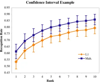
Figure 3 shows the 95% confidence intervals obtained in the manner just described for ranks 1 through10. To keep the figure readable, the confidence intervals for only the PCA algorithm using Mahalanobis and L1 distance are shown. Keep in mind that these are pointwise intervals for each rank that are not adjusted for multiple comparisons. These plots are elaborations of the CMS plots commonly used in the FERET evaluation with the notable exception that now intervals rather than single curves are shown.
Both the distributions and confidence intervals call at-tention to the differences between PCA using Mahalanobis distance, L1 and the other distance measures. For exam-ple, based upon the overlapping confidence intervals shown in Figure 3, one might be drawn to conclude there is no significant difference between PCA using L1 versus PCA using Mahalanobis distance. However, as the next section will show, there are more direct and discriminating ways to approach such questions, and simply looking to see if con-fidence intervals overlap can be somewhat misleading.
7.2. Hypothesis Testing
The question typically asked is: Does algorithm A per-form better than algorithm B? This gives rise to a one sided test of the following form. Formally, the hypothesis being
Figure 3. The 95% confidence intervals for PCA using L1 and Mahalanobis distance.
tested and associated null hypothesis are:
H1 The recognition rateR
kfor algorithm A is higher than for algorithm B.
H0 The recognition rates are identical for both algorithms.
To establish the probability of H0 a new statistic D
k
(A;B)is introduced that measures the signed difference in recognition rates: D k (A;B)=R k (A) R k (B) (16)
The same Monte Carlo method used above to find the dis-tribution for R
k may be used to find the distribution for D
k
(A;B). Figure 4 shows these distributions for the PCA algorithm using three pairs of distance measures: Maha-lanobis minus L1, L1 minus L2 and L2 minus angle. For the first two differences, the separation of the recognition rate distributions in Figure 1 suggests the difference may be significant.
Figure 4 accentuates this conclusion. The third compar-ison, L2 to angle, is included to illustrate howD
k behaves for algorithms that are not substantially different. Table 3 shows the probabilities for the observed differences given H0. With very high confidence, H0 may be rejected in favor of H1 for the first two comparisons, and not for the third.
At first glance it might appear wise to carry out all42 possible pairwise tests usingD
k. However, doing so invites false associations. The common practice of rejecting H0 at probability level0:05implies that it is very likely that one will mistakenly reject H0 a few times. Multiple comparison procedures could be employed to remedy this problem, but
Figure 4. Rank 1 distribution for recognition rate difference. Alg. A Alg. B P(D 1 (A;B)<0) Mah. L1 0:0035 L1 L2 0:0003 L2 Angle 0:9014
Table 3. Probability of H0 at rank 1 given ob-served difference in recognition rate.
a full analysis of variance [2] would provide a richer model for inference. In future work we plan to pair the analysis of variance model with the permutation inferential paradigm to provide a complete analysis of such experimental data. In lieu of such a procedure, looking at individual performance measures and making a small set of salient pairwise tests is a reasonable strategy.
7.3. Balanced versus Unbalanced Sampling
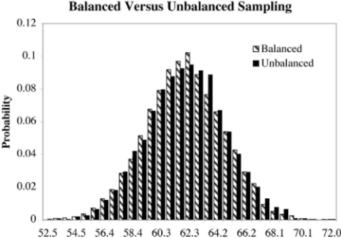
Section 7 stated that sampling may be done in either a balanced or unbalanced fashion. Does the distinction mat-ter in our context? Figure 5 shows the result of one such comparison: the recognition rate probability distribution for the PCA algorithm using Mahalanobis distance obtained us-ing balanced versus unbalanced samplus-ing. The distinction does not appear to matter: the two distributions are essen-tially indistinguishable. The other distributions presented above were also essentially unchanged when unbalanced sampling was compared to balanced. More work is needed to fully explore the implications of the two alternative sam-pling methods, but at least using the definitions of balanced versus unbalanced sampling introduced above, the distinc-tion appears to matter little.
Figure 5. Distributions obtained using bal-anced versus unbalbal-anced sampling.
8. Summary and Conclusions
Face recognition algorithms using PCA and LDA sub-spaces have been compared over640FERET face images. Each subspace variant has been tested using several com-mon distance metrics. Probability distributions for recog-nition rates and differences in recogrecog-nition rates relative to different choices of gallery and probe images have been cre-ated using a Monte Carlo sampling method.
Somewhat surprisingly given the strength of the LDA al-gorithm relative to the PCA alal-gorithm in the FERET eval-uations [17], on our tests the LDA algorithm performs uni-formly worse than PCA. Further work is required to fully explain why, but differences in LDA training procedures are likely to prove important. Zhao trained using synthetically altered imagery to boost the training samples per class, a process not repeated here.
The Monte Carlo approach for establishing confidence intervals on recognition rate is similar to that of Micheals and Boult [13] while avoiding their algebra and their re-liance on variance estimates and normal approximations. Future work will more fully explore linkages between our approach and theirs.
Acknowledgements
This work supported by the Defense Advanced Research Projects Agency under contract DABT63-00-1-0007.
References
[1] P. Belhumeur, J. Hespanha, and D. Kriegman. Eigenfaces vs. fisherfaces: Recognition using class specific linear
projec-tion. IEEE Transactions on Pattern Analysis and Machine Intelligence, 19(7):771 – 720, 1997.
[2] P. Cohen. Empirical Methods for AI. MIT Press, 1995. [3] Duane M. Blackburn and Mike Bone and P. Jonathon
Phillips. Facial Recognition Vendor Test 200. http://www.dodcounterdrug.com/facialrecognition/frvt2000/ frvt2000.htm, DOD, DARPA and NIJ, 2000.
[4] R. O. Duda, P. E. Hart, and D. G. Stork. Pattern Classifica-tion. John Wiley & Sons, second edition edition, 2001. [5] B. Efron and G. Gong. A Leisurely Look at the Bootstrap,
the Jackknife, and Cross-validation. American Statistician, 37:36–48, 1983.
[6] FERET Database. http://www.itl.nist.gov/iad/humanid/feret/. NIST, 2001.
[7] R. Haralick. Performance Characterization in Computer Vi-sion. CVGIP, 60(2):245–249, September 1994.
[8] J. Ross Beveridge. The Geometry of LDA and PCA Classi-fiers Illustrated with 3D Examples. Technical Report CS-01-101, Computer Science, Colorado State University, 2001. [9] K. W. Bowyer and J. Phillips (editors). Empirical
evalua-tion techniques in computer vision. IEEE Computer Society Press, 1998.
[10] M. A. Turk and A. P. Pentland. Face Recognition Using Eigenfaces. In Proc. of IEEE Conference on Computer Vi-sion and Pattern Recognition, pages 586 – 591, June 1991. [11] M. Kirby and L. Sirovich. Application of the
Karhunen-Loeve Procedure for the Characterization of Human Faces. IEEE Trans. on Pattern Analysis and Machine Intelligence, 12(1):103 – 107, January 1990.
[12] P. Phillips, H. Moon, S. Rizvi, and P. Rauss. The FERET Evaluation Methodology for Face-Recognition Algorithms. T-PAMI, 22(10):1090–1104, October 2000.
[13] Ross J. Micheals and Terry Boult. Efficient evaluation of classification and recognition systems. In IEEE Computer Vision and Pattern Recognition 2001, page (to appear), De-cember 2001.
[14] H. Wechslet, J. Phillips, V. Bruse, F. Soulie, and T. Hauhg, editors. Face Recognition: From Theory to Application. Springer-Verlag, Berlin, 1998.
[15] J. J. Weng and D. Swets. Face recognition. In Biometrics: Personal Identification in Networked Society. Kluwer Aca-demic Publishers, 1999.
[16] W. S. Yambor. Analysis of pca-based and fisher discriminant-based image recognition algorithms. Master’s thesis, Colorado State University, 2000.
[17] W. Zhao, R. Chellappa, and A. Krishnaswamy. Discriminant analysis of principal components for face recognition. In In Wechsler, Philips, Bruce, Fogelman-Soulie, and Huang, edi-tors, Face Recognition: From Theory to Applications, pages 73–85, 1998.
[18] W. Zhao, R. Chellappa, and P. Phillips. Subspace linear dis-criminant analysis for face recognition. In UMD, 1999.