Modeling and Verification
Saikat Mukherjee1, Hasan Davulcu2, Michael Kifer1, Pinar Senkul3, and Guizhen Yang1
1 Department of Computer Science, Stony Brook University, Stony Brook, NY 11794-4400, USA
{saikat,kifer,guizyang}@cs.stonybrook.edu
2 Department of Computer Science & Engineering, Arizona State University, Tempe, AZ 85287-5406,USA
3 Department of Computer Engineering, Middle East Technical University, Ankara, 06531, Turkey
Abstract. A workflow is a collection of coordinated activities designed to carry out a well-defined complex process, such as trip planning, student registration, or a business process in a large enterprise. An activity in a workflow might be performed by a human, a device, or a program.Workflow management systems(or WfMS) provide a framework for capturing the interaction among the activities in a workflow and are recognized as a new paradigm for integrating disparate systems, including legacy systems. A large workflow system might involve many disparate activities that are coordinated in complex ways and are subject to many constraints. Thus, modeling such systems and ensuring that they perform according to the specifications is not an easy task. To be able to analyze the properties of workflows, the latter must be specified using a formalism with well-defined semantics. The popular formalisms in this area are the various logics, Petri Nets [1,35], Event-Condition-Action rules [23,15], and State Charts [36]. In this chapter we survey and compare a number oflogic-based formalisms that were proposed in the literature.
5.1
Introduction
A workflow is a collection of coordinated activities designed to carry out a well-defined complex process, such as trip planning, student registration, or a business process in a large enterprise. Business processes are represented as sets of tasks, where each task carries out some well-defined activity. An activity can be as simple as reading and approving a document or it may involve a complex process of its own. An activity can be completely auto-mated or may involve manual interaction. A workflow management system (WfMS) is a set of tools for defining, analyzing, and managing the execution of workflows. To design a workflow, one uses a workflow modeling language (often through a graphical interface) to specify the tasks, the flow of data, the control flow, and a set of constraints on the execution. A WfMS includes
an interpreter that understands workflow specifications, can analyze them for correctness, and schedule workflow events accordingly. During the execu-tion, a WfMS interacts with the participants in the workflow and invokes the necessary applications when required.
Prior to the advent of workflow management systems, business processes were automated in an ad hoc manner and each system involved one of a kind solution. It was therefore hard to deploy a workflow system and also to adapt it to a changing business environment. A WfMS can substantially reduce the cost of business process engineering and maintenance through
• reduced operating costs — by driving down the cost per transaction
• improved productivity — by eliminating routine and repetitive tasks
• better analysis, which simplifies the job of creatingcorrectworkflows and leads to higher quality designs
• improved change management — using the tools provided by a WfMS, organizations can modify workflow specifications much more easily and quickly adapt to changes in the business environment
• better decision support — the tools provided by a WfMS can be used to analyze the workflow, flag inefficiencies, and verify that the workflow specification meets its goals.
The development of robust workflow management systems is one of the most important challenges in today’s information systems. Collaborative design, health-care, and Web services are some examples of applications that require automated workflow management. Though traditional applications have kept researchers busy,Web services are driving the renewed interest in this area. From the workflow point of view, a Web service is a task with a well-defined interface. A number of proposals exist to standardize the various parts of this interface (for example, UDDI [27], WSDL [26], DAML-S [3]). The promise of Web services is that the standardized interface makes it possible to combine disparate services into complex workflows, and thus many issues that arise in the context of workflows are pertinent to Web services. In addition, Web services present new, unique challenges. First, because different services are under the control of different organizations, it can no longer be assumed that they all cooperate. Therefore, it becomes necessary to be able to model workflows whose tasks might execute in an adversarial environment. One work in this vein is [14]. Related to this is the potential need to negotiate services. As consumers, we do not always accept the first offer and try to find a better deal — often from the same merchant. Thus, the ability to negotiate is another unique aspect of a Web service, which brings us into the realm of agent-based systems [22,31].
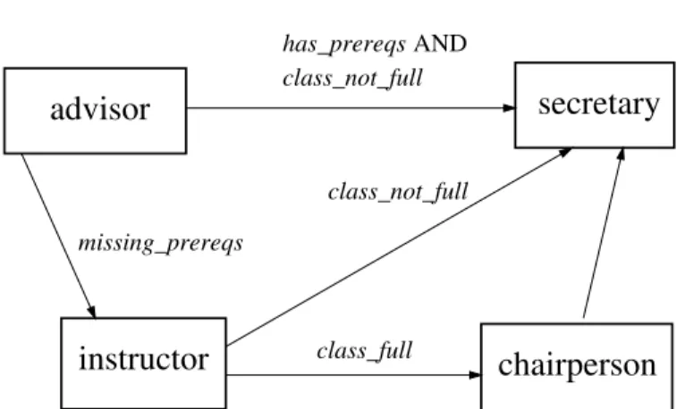
At its core, a workflow is a process, and, thus, a WfMS requires a pro-cess specification language. Figure 5.1 is an example, borrowed from [5], of a workflow that determines whether a student is allowed to register for a course. The process definition is comprised of different tasks, which perform the job of an advisor, instructor, etc. (pertaining to the registration process).
class_not_full
AND
instructor
class_fullchairperson
missing_prereqs
class_not_full
advisor
secretary
has_prereqs
Fig. 5.1. Example of a registration authorization workflow
For instance, the taskadvisordetermines whether the student has the prereq-uisites for the course;instructor may give the student permission to attend the course if the class is not full, even if the student does not satisfy the pre-requisites; chairperson can give permission to attend the course even if the class is already full, but provided that the student satisfies the prerequisites. The tasksecretarymodels the secretary who enters the registration informa-tion into the system. A WfMS manages the registrainforma-tion process by creating an instance of this process definition, which in turn contains an instance for each task. The edges connecting the activities represent the flow of control between the activities, and the labels represent transition conditions. The control flow and transition conditions are enforced by the WfMS at run time. The problem of scheduling events that arise during the execution of a workflow can be hard both from the point of view of computational complex-ity and also algorithmically. A business workflow can include dozens and even hundreds of tasks, which might be related through a large number of global dependencies that cannot be easily represented using a control flow graph such as that in Figure 5.1. Typical global dependencies are of the form “if events A and B occur, then event C must not occur” or “if A occurs, then it must happen before B.” Apart from scheduling, workflow specifications might need to beverified. One problem here is whether the constraints are consis-tent with each other or with other parts of the specification. If they are not, the workflow cannot be scheduled. A related problem is to find out whether a certain property is ensured by the workflow specification. For instance, a mail-order workflow might need to ensure that product is not shipped prior to receiving an authorization from a credit card company. This constraint might or might not follow from the already existing constraints. Of course, we could simply add this constraint to those existing constraints, but then we would have to waste time enforcing it when a verification procedure might
determine that this constraint is automatically enforced if the rest of the constraints are obeyed.
The need for formal methods in workflow modeling and verification has been widely recognized [2,20] and a number of formal frameworks have been proposed. These includes Event-Condition-Action rules (triggers) [16,18,23], the various logic-based methods [4,5,10,13,14,21,28,29], Petri Nets [1,34,35], and State Charts [36].
The past few years have seen progress in both the implementation and foundational aspects of workflow management systems. However, commercial systems offer only relatively rudimentary modeling capabilities. Specification of global intertask constraints is still difficult, and verification tools are vir-tually absent. These limitations force application developers to embed the enterprise logic deep into the code, which leads to considerable implementa-tion effort and high maintenance overhead.
In this survey, we discuss a number of logic-based approaches to modeling and managing workflows. In particular, we are interested in the expressive power of the approaches as well as their applicability to the problems of scheduling and verification of workflows. In Section 5.3, we discuss a proposal [4] based on temporal logic [17]. Section 5.4 presents a related approach, which is formalized using a specially devised event algebra [29]. Section 5.5 reviews workflow modeling techniques [6,13], whose underlying formalism is Concurrent Transaction Logic [7]. Finally, Section 5.7 concludes the chapter and provides a brief comparison of the approaches discussed.
Though we were striving for completeness, limitation of space and scope forces us to leave out some logic-based approaches, such as [5], which is based on Action Logic and triggers; ACTA [10], which attempts to formalize extended transaction models in first-order predicate logic; and Vortex [18], which uses model checking techniques to verify properties of workflows. We briefly survey these works in Section 5.6.
5.2
Preliminaries
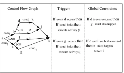
A workflow can be modeled using one or more frameworks, and each frame-work can use one or more of the formalisms, such as logic, Petri Nets, etc. The most common frameworks are illustrated in Figure 5.2. These include control flow graphs,global temporal constraints, and triggers.
Note that the boundary between the frameworks in Figure 5.2 is somewhat subjective and can vary from one approach to the next. The control flow graph can be represented as a set of constraints, and some global constraints can be represented directly in the control flow graph. Likewise, some constraints can be described as triggers, and some triggers can be modeled as constraints.
Control Flow Graph b g f i j h d If event then Ifcond holds then
execute activity
Ifeventg occursthen Ifcond holdsthen
execute activity q cond cond1 4 occurs d p AND OR k
Triggers Global Constraints
If eandiare both executed
then e must happen before i
then
is ever executed
If d
must also happen
g cond3 a cond2 c OR e
Fig. 5.2. Frameworks for specifying workflows
5.2.1 Modeling Concepts
The control flow graph is the primary technique used in commercial work-flow systems. A graph specifies the initial and final activity in a workwork-flow, the successor activities for each activity in the graph, and whether these successors must all be executed concurrently, or it suffices to execute just one branch nondeterministically. Arcs in a control flow graph can be labeled withtransition conditions. The condition applies to the current state of the workflow. When the task at the tail of an arc is completed, the task at the head can begin only if the corresponding transition condition evaluates to true. The control flow graph is most appropriate for depicting thelocal inter-task dependencies of the activities in a workflow. However, their limitation is that they cannot be used to specifyglobal intertask dependencies between workflow tasks.1Dependencies (also known asconstraints—we shall use these two terms interchangeably) provide a more general framework for specifying workflows. In particular, the precedence relationship that underlies the con-trol flow graph is just another kind of constraint. Less obvious is the fact that both the AND-nodes and OR-nodes can be modeled as constraints (see Section 5.4). Nevertheless, separating global constraints from the graph is useful both as a pragmatic modeling technique and as a way to find more efficient scheduling algorithms (see Section 5.5). Triggers are another way of specifying control flow dependencies. Like control flow graphs, triggers are limited in their ability to specify global dependencies among tasks. They are 1 We shall see in Section 5.5 that this is theoretically possible, but practically not feasible, because compiling constraints into a control flow graph can lead to an exponential explosion of the graph. Thus, constructing such graphs manually is not an option.
also not sufficiently expressive when it comes to specifying alternatives in workflow execution (OR nodes).
The use of intertask dependencies for workflow modeling was first pro-posed in [25] and has since become a basic staple of workflow modeling works. The typical constraints on event occurrence and ordering are
• e1→e2(occurrence): Ife1occurs, then so must bee2. No specific ordering is implied.
• e1< e2(order): If bothe1ande2occur, thene1must be scheduled before
e2. This constraint is trivially satisfied if only one of the events occurs. A workflow specification in the form of constraints, control flow graph, or triggers is analogous to a database schema. A concrete workflow executing according to that specification is called aworkflow instanceand is analogous to database instances. Execution of a particular workflow instance is typi-cally defined in terms of itsevent history, i.e., the sequence of “significant” events (see below) that have occurred during the execution. The semantics of constraints is also defined in terms of these histories. For instance,e1< e2 is satisfied in a given history if and only ife1 occurs prior toe2in that history. The workflow scheduler is a module in a WfMS that examines the in-coming sequence of events, generated by the execution of workflow activities, and schedules them in a certain order so that all of the given constraints would be satisfied. Alternatively, the scheduler mightproactively construct a concise model of all possible executions. In this case, scheduling is essentially performed at compile time with only trivial decisions left to be made at run time. Systems that follow the former approach are described in Sections 5.3 and 5.4. An example of the latter approach appears in Section 5.5.
Many formal approaches to workflow modeling and scheduling (in par-ticular, those surveyed in this chapter) rely on some or all of the following assumptions:
Significant events: Workflow tasks are modeled as black boxes that emit significant events. A significant event is an abstraction that represents real events that occur during the workflow execution, in which the scheduler might be interested because they need to be put in a certain order (say, because they are mentioned in a constraint). Negation of a significant evente (denoted as ¯eor ¬e) is also frequently used. The event ¯eis said to occur if the eventenever occurs in the execution.
A significant event can be one of the standard events, such as start, precommit, commit, and abort, whose semantics is known in advance, or it might be application-specific, for example, sending a message to another task. Certain constraints associated with the standard events follow from their a priori semantics. For instance,startT must precede any other event of the same task (startT < eventT) and a termina-tion event, commitT or abortT, must be the last event in any task (eventT < commitT,eventT < abortT). Similarly,commitT andabortT
cannot happen in the same execution of a workflow (commitT →abortT andabortT →commitT).
For application-specific events, the workflow designer typically speci-fies constraints explicitly, as they depend on the application domain. For instance, the business rules of an enterprise might require that if
task shipP roduct commits, then task conf irmP ayment must commit
prior to that (i.e., commitshipP roduct → commitconf irmP ayment and
commitconf irmP ayment< commitshipP roduct).
Unique event property: No event can occur more than once in the ex-ecution of the same instance of a workflow. The rationale behind this assumption is that an event is associated with a task and a timestamp, so it cannot occur more than once in any given execution sequence. This assumption does not preclude events of the sametypefrom occurring more than once. For instance, a task can send a message to another task several times. However, if multiple events of the same type are allowed to occur, this presents a problem for the constraint specification language. For instance, how can one specify that a response to a request must follow the request? Such a statement requires that events have properties (such as event ID and context), which can be used to match a response to the corresponding request.
Forcible, rejectable, and delayable events: Some formalizations assume that significant events have certain attributes that the scheduler can use in making its decisions:
• Forcible: an event is forcible if the scheduler is permitted to make the event happen. Of course, constraints must be satisfied, but the decision whether or not to start such an event is the scheduler’s pre-rogative. For example,abortandstartare forcible, since the scheduler can always abort a running task or start another task. IfstartT1 →
abortT2 is a constraint and taskT1has already started, the scheduler might decide to force the abort ofT2to satisfy the constraint. In contrast, the scheduler might not be allowed to send messages to tasks on behalf of other tasks, so such events are not forcible.
• Rejectable: an event is rejectable if the scheduler is free to prevent this event from happening. For example, the scheduler has the discretion to prevent any task from committing its work or from starting (again, subject to constraints).
To see where this is useful, suppose that the constraint isstartT1 <
commitT2 andT2has already committed. If the eventstartT1 arrives later, the scheduler can still ensure that the constraint is satisfied by rejecting this event.
• Delayable: an event is delayable if the scheduler is free to delay the ex-ecution of that event. For instance, if a task has requested to commit, the scheduler might decide to delay scheduling this event.
Delaying is typically done to make sure that certain constraints are satisfied. For example, if startT1< commitT2 is a constraint andT2
requests to commit, the scheduler might decide to delay this event untilT1 starts.
5.2.2 Example
To illustrate the different notions of events and constraints introduced in this section, let us consider an airline reservation workflow. The tasks associated with this workflow are
• Buy: buying an airline ticket
• Book: booking a car
The significant events associated with the taskBuyarestartBuy,commitBuy, andabortBuywhich, respectively, start, commit, and abort the taskBuy. The significant events associated with the taskBook arestartBook,commitBook,
abortBook, andcancelBookwhich, respectively, start, commit, abort, and can-cel the task Book. Observe that although booking a car can be canceled, buying an airline ticket cannot be canceled. A dependency associated with this workflow is thatBuy commits only if Book commits. This can be rep-resented as the occurrence constraint commitBuy → commitBook. Also, if the Buy aborts then Book should also abort. This can be similarly repre-sented as the constraintabortBuy→abortBook. Another dependency in this workflow is that if both Book and Buy commit, then Book commits be-fore Buy. This can be represented as the order constraint commitBook <
commitBuy. Yet another dependency in the workflow is that Book is can-celed if and only if Book commits and Buy aborts. This can be modeled as the pair of occurrence constraints cancelBook → (commitBook∧abortBuy) and (commitBook∧abortBuy) → cancelBook. All of the above mentioned events are delayable by the scheduler. If the event commitBuy happens be-forecommitBook, then the scheduler can delay the acceptance ofcommitBuy to satisfy the dependency that Book commits before Buy. An example of a forcible event iscancelBook because the scheduler has to force that event to satisfy constraints whenBook commits andBuyaborts. On the other hand, if Buy aborts and the eventcommitBookis to be scheduled, then the scheduler has to reject commitBook to satisfy the dependencies. Thus, commitBook is an example of a rejectable event.
5.2.3 The Role of Logic
Logic plays different roles in different formalisms surveyed in this chapter. In [4], Temporal Logic serves only as a specification medium. It provides both the syntax and the semantics for the constraints. However, the workflow scheduler works directly with automata — the low-level representation of temporal constraints.
In contrast, logic is much more closely interwoven into the frameworks of [13] and [29]. In both formalisms, logic is a primary means of specifying
the workflows. In addition, the workflow scheduler can be implemented as a particular strategy in the proof theory of the logic. In [29], the proof theory is based on theresiduation operator, and the scheduler uses this operator to make scheduling decisions. In [13], the scheduler depends on a preprocess-ing step after which the proof theory of Concurrent Transaction Logic [7] is employed directly to make scheduling decisions.
5.3
Modeling Workflows with Temporal Logic
In [4], Attie et al. proposed modeling workflows as a set of intertask de-pendencies. Both local and global constraints (beginning of Section 5.2) can be modeled in this way, and, therefore, the control flow graph is not repre-sented explicitly.2The tasks in a workflow are described in terms of significant events. A typical event is the beginning or termination of a task, but it can also be sending an email to the boss, printing a report, etc.
When an event is received for execution, it is checked against every depen-dency and, based on that, the event might be accepted, rejected, or delayed and scheduled later. The dependencies are specified as formulas in Computa-tional Tree Logic (CTL) [17]. The scheduler enforces these dependencies by converting them into automata and ensuring that the sequence of scheduled events is accepted by all of these automata. In this way, the automata provide a low-level medium for the scheduler to work with, and the logic serves as a high-level specification medium.
This work does not explicitly deal with verification issues, such as whether the given set of constraints implies some other constraints. Of course, stan-dard high-complexity model-checking techniques can be used here, but the interesting question is whether the implication of workflow dependencies can be tested more efficiently due to the specialized form of these constraints.
5.3.1 Formalization
Formalization makes all of the assumptions listed in Section 5.2: workflows are modeled as streams of significant events such asstart,precommit,commit, andabort; the unique event assumption holds; and events can be delayable, rejectable, or forcible.
A workflow is specified as a set of dependencies over the events associated with the tasks. If e1, e2, ..., en are the significant events associated with a number of tasks, then a dependency D involving these events is denoted asD(e1, e2, ..., en). Computational Tree Logic (CTL) is used to specify these dependencies. For instance, the order dependency,e1< e2, is specified in CTL as A(e2 → A¬e1), i.e., the following is true on every path: Ife2 occurs thene1will not occur later on any continuation of that path. A dependency,
D, specified in CTL, is compiled into a finite state automatonAD, which is a tuplehs0, S, Σ, ρi, where:
• S is a set of states.
• s0is the initial state.
• Σis a set of event expressions, which can have one of the following forms:
– a(e1, ..., en), wheree1, ..., enare events. This expression says that the eventse1, ..., enareacceptedbyADand scheduled for execution. Each
ei is a significant event of some task.
– r(e1, ..., en), wheree1, ..., en are events. This expression says that the eventse1, ..., enarerejectedbyAD. The automatonADis constructed so that the rejection takes place precisely when the execution of these events (in any order) would violate the dependencyD.
– σ1 k... kσn, whereσi ∈Σ. This expression specifies that the event expressionsσ1, ..., σn are run concurrently in an interleaved fashion.
– σ1;...;σn, whereσi ∈Σ. In this expression, the operationsσ1, ..., σn are run insequence.
• ρ⊂S×Σ×S is the transition relation.
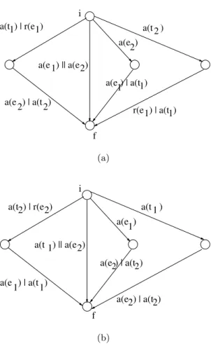
Figure 5.3a is an automaton for the occurrence dependency e1 → e2. Here, we uset1 to denote the significant event of termination (i.e., abort or commit) of task 1 andt2to denote the termination event for task 2. Symbols
e1 and e2 are used to denote other nontermination events. Because of the special semantics of termination events, no significant events from a task i
can arrive once the eventti has arrived, andti must be scheduled last. The symbol| indicates choice —either event can cause the correspond-ing transition. This should be contrasted with the event combinator k. For instance, an arc labeled witha(e1)ka(e2) means thatboth events,e1ande2, must occur and the corresponding state transition can happen in one of two ways: Either by scheduling a(e1) first and a(e2) next or by scheduling these events in the reverse order.
The initial state in every automaton is denoted by i and the final state by f. Every path from the initial state to the final state corresponds to a way in which the dependency can be satisfied. Formally, for any dependency automaton,AD, apathπis a sequence of event expressionsσ1... σnsuch that there are statess1, s2, ..., sn−1, sn inAD, where
• s1is the initial state ofAD;
• sn is a final state ofAD; and
• for each i= 1, ..., n−1: (si, σi, si+1)∈ ρD, where ρD is the transition relation ofAD (i.e., each σi is a legal transition from state si to si+1 in
AD.
Figure 5.3a shows some sequences of events that satisfy the dependencye1→
e2:
• a(t1)a(e2) — termination of task 1 followed by acceptance ofe2.
• a(e1)a(e2) and a(e2)a(e1) — because a(e1)k a(e2) is a label on one of the arcs, which means that executing e1 and e2 in any order can cause the corresponding transition.
• a(e2)a(t1) — acceptance ofe2 followed by termination of task 1.
• a(t2)r(e1) — termination of task 2 followed by rejection ofe1.
• a(t2)a(t1) — termination of task 2 followed by termination of task 1.
• Other event sequences that satisfy the above dependency arer(e1)a(t2),
a(t1)a(e2), anda(e2)a(e1). Note that in the first case, the evente1 does not occur in the history, so the dependencye1→e2is satisfied trivially. In the last case, the events occur in the reverse order. However, because both of them occur, the constraint is satisfied once again, as it only implies occurrence, not order.
Similarly, Figure 5.3b is an automaton for the order dependencye1< e2. The sequence of events a(t1)a(e2) is accepted by both automata, because each automaton has a path consistent with this sequence of events. However, the sequence a(e1)a(t2) is accepted by the automaton only for e1 < e2, becausea(e1)a(t2) does not correspond to a legal execution sequence in the automaton for the dependencye1→e2.
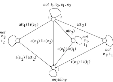
We can now define what it means for a sequence of events to be a legal execution. To simplify matters, we augment the dependency automata with additional arcs, namely, we add a self-loop to every state in each automaton. Ifn is a node in an automaton, then the corresponding self-looping arc has
nas its beginning and end, and it is labeled by every event expression of the forma(event) orr(event) such thateventisnotmentioned on other outgoing arcs ofn. (Note that if, say,a(e2) is mentioned on an outgoing arc ofnthen neither a(e2) nor r(e2) can occur on the self-looping arc.) The idea is that events that are not mentioned on these outgoing arcs leave the automaton in staten. In addition, we also make the initial state of the automaton into an accepting (final) state. The automaton of Figure 5.3a transformed in such a way is depicted in Figure 5.4. In this figure, a label such as “not e2, t2” means that the transition along that arc can be caused by any event expression that does not mentione2ort2. For instance, neitherr(e2) nora(e2) can cause the transition, buta(t1) orr(e1) can.
We now define a sequence of events as alegal execution path if it is ac-cepted by every such augmented automaton. Note that due to the unique event assumption, an event can be mentioned in at most one event expres-sion on the execution path.
5.3.2 Scheduling
In the previous subsection, we defined execution paths as sequences of event expressions. However, the scheduler receives sequences of events rather than event expressions. Thus, given a sequence of events, seq, the work of the
r(e1) | a(t1) a(e 1) | a(t1) a(t 2 ) a(e 2) a(t1) | r(e1) a(e ) | a(t 2) ) 2 ) || a(e 1 a(e 2 i f (a)
a(t2) | r(e2) a(t 1 )
a(e1) a(e1) | a(t1) a(e2) | a(t2) ) 2 ) || a(e 1 a(t i f ) a(e ) | a(t2 2 (b)
Fig. 5.3. Dependency automata: (a) Automaton for the dependencye1→e2, (b) Automaton for the dependencye1< e2
scheduler is to find a legal execution path,π, such that the events mentioned in the expressions inπare all and the only events that occur inseq. If every automaton is of size N and there are m automata, then one can build a product automaton of sizeNm. Unfortunately, this might be unacceptable for workflows that have many constraints.3To avoid this state explosion problem, the individual automata are checked at run-time, as explained below. The worst time complexity of run-time scheduling is still exponential. However, it is believed that the worst case does not occur in practice [4].
The global state of the scheduler is a tuple whose components are the local states of the dependency automata — one state per automaton. The 3 Observe that in this framework, even the control flow graph is represented as a
anything not not not e , t t , t , e , e not 1 2 1 2 e , t e , t1 1 1 1 2 2 r(e ) | a(t1)1 a(t1) | r(e1) a(e1) | a(t1) a(t 2 ) a(e 2) ) | a(t2) ) 2 ) || a(e 1 a(e 2 i f f a(e
Fig. 5.4.Automaton of Figure 5.3a augmented with self-looping transitions
initial global state is a tuple of the initial states of these automata. When an event, e, arrives, the algorithm tries to construct an event sequence, π, which is accepted by everyaugmented automaton, such thatπincludeseand (possibly) some of the events that have arrived previously but have not yet been scheduled (these are calleddelayed events).4In addition, each event on the path must occur at most once (for example, a(e2) and r(e2) count as multiple occurrences of event e2). If such a path cannot be found, then the scheduler delays the execution of evente.
Consider the dependencies e1→e2 ande1 < e2 with the automata A→ andA<, respectively, shown in Figure 5.3. LetA0→ andA0< be the augmen-tations of these automata. Augmentation forA→is shown in Figure 5.4, and augmentation of A< is constructed similarly. Let e1 be an event submitted to the scheduler. Because there is no path in both automata that begins by either accepting or rejectinge1, the scheduling ofe1has to be delayed. Now suppose that event e2 is submitted to the scheduler. Two execution paths can be found inA→ that accept both e1 and e2: a(e2)a(e1) and a(e1)a(e2). The only path inA< that accepts bothe1 ande2 isa(e1)a(e2). However, in
a(e1)a(e2), the order of events is different from the patha(e2)a(e1) in A→.
Thus, the only legal execution path isa(e1)a(e2) — the scheduler can execute
e1 followed bye2 and satisfy both constraints.
4 Note that e might not be mentioned in a nonaugmented automaton, so there would be no guidance as to what to do when such an event arrives. Anaugmented automaton would simply discard such an event.
5.4
Modeling Workflows Using Event Algebra
In [29], Singh defines an algebra, that is suitable for reasoning about con-straints over an incoming stream of events. This algebra is sufficiently ex-pressive to represent very general temporal intertask dependencies, including control flow graphs. But conditions on transitions between tasks in such a graph cannot be expressed.5A scheduling algorithm starts with an expression that represents the entire set of constraints and then chips away at these ex-pressions (orresiduates in the terminology of [29]) as it schedules the arriving events.
Though event algebra is an elegant solution for the problem at hand, it is unclear whether it can model subworkflows or be used to verify workflow properties such as whether a given set of constraints has redundancy in it or whether a constraint is implied by a set of constraints.
5.4.1 Formalization
Execution of a workflow relies on the notion of significant events produced by the tasks that comprise the workflow. Examples of such events arestart, precommit, commit, andabort. A workflow is specified as a set of dependencies among these significant events. The dependencies are represented as event expressions in the algebra.
The set of symbols that represent significant events is denoted byΣ. This set does not need to be finite. Anatomic event expression is either an event symbol fromΣ or its negation. Ife∈Σ, then its negation is represented as ¯
e; it represents the assertion that e does not occur in the execution of the workflow. We will use lowercase letters to represent atomic events and capital letters for more complex event expressions.
The language ofevent expressions, denoted byE, is defined as follows:
• Γ ={e,¯e|e∈Σ} ⊆ E.
This just states that atomic events are event expressions. We useΓ to represent the set of atomic events.
• We distinguish two special event expressions : 0 and >in E. The event 0 represents the event expression that is always false and the event >
represents the expression that is always true.
• If E1, E2 ∈ E, then E1·E2 ∈ E. The operator “·” denotes sequencing, i.e., the event expression E1 followed by the event expression E2 (not necessarily immediately).
• If E1, E2 ∈ E, then E1+E2 ∈ E. The operator “+” denotes choice or disjunction. The expression says that either the event expressionE1must occur orE2.
5 Note that although [4] does not discuss scheduling in the presence of such con-ditions, they can at least be expressed in temporal logic.
• IfE1, E2 ∈ E, then E1|E2 ∈ E. The operator “|” means conjunction. It denotes an event expression that represents bothE1 andE2 occurring in any order.
The event algebra uses denotational style semantics where an event ex-pression represents a set of legal traces. Alegal trace(which we will often call just atrace) is a sequence of atomic events where
• each event symbol occurs at most once in the same trace (the unique event assumption);
• an event and its negation cannot occur in the same trace; and
• for eache∈Σ, eithereor ¯eoccurs in the trace.
Note that if ¯e occurs in a trace, then the exact placement of this symbol is immaterial: If an event does not occur in a trace, then this remains true regardless of where ¯ewas actually placed in the trace.
An event expression represents a constraint on the execution and the set of traces it represents are those that satisfy this constraint. For example,eis a constraint that says that the eventemust occur, and the corresponding set of traces contains precisely those that have ein them. The event expression
e·f¯is a constraint that says that after eoccurs, then f cannot occur any longer (i.e., iff occurs at all, it must occur beforee). The corresponding set of traces includes those that haveeand either have no f orf occurs before
e.
The set of traces (ordenotation) for an event expressionE is denoted by [E]. Given a set of atomic events, Γ, UΓ ⊂Γ∗∪Γω is the set of all finite (Γ∗) and infinite (Γω) traces over the language Γ, i.e., sequences of events that satisfy the three conditions given above.6The denotations of the various event expressions are defined as follows:
• [e] ={τ ∈UΓ |e∈τ, i.e., eoccurs inτ}
• [0] =∅, that is, no trace satisfies the expression 0.
• [>] =UΓ, that is, every trace satisfies the expression >.
• Sequencing: [E1·E2] ={ντ ∈UΓ | ν ∈[E1] andτ ∈[E2]}, that is the resulting trace is obtained by concatenation of the traces ofE1 andE2.
• Disjunction: [E1+E2] = [E1]∪[E2].
• Conjunction: [E1|E2] = [E1]∩[E2].
For an event expression E∈ E and a traceτ ∈UΓ, τ |=E denotes satisfia-bility of the event expression E by the traceτ, i.e., the fact thatτ∈[E].
Consider a travel workflow where one attempts tobuy an airline ticket and book a car. The constraint is that either both tasks succeed or none succeeds. The other constraint is that buy cannot be canceled whereasbook can. This workflow can be formulated in this algebra as the following set of dependencies:
6 Note that ifΣis finite, then there can be no infinite legal traces due to the unique event assumption.
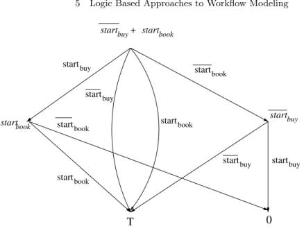
• D1:startbuy+startbook: Ifbuy starts thenbook must also start.
• D2:commitbook+commitbuy+commitbook·commitbuy: If bothbook and buy commit thenbook commits beforebuy.
• D3:commitbuy+commitbook: Taskbuy commits only ifbook commits.
• D4:commitbook+commitbuy+startcancel: Ifbookcommits andbuy does not then startcancel.
• D5:startcancel+commitbuy|commitbook: Start cancel only ifbook com-mits andbuy does not.
This workflow is satisfied by several traces some of which are startbuystartbook
commitbookcommitbuy, startbookstartbuystartcancel, and startbookstartbuy
commitbookcommitbuy.
5.4.2 Scheduling
Given a set of dependencies specified as a set of event expressions, the job of the scheduler is to find traces that satisfy the dependencies. The scheduler starts with an event expression that represents all dependencies. An incoming event is scheduled when this act is guaranteed not to break the dependen-cies, regardless of which events will arrive in the future. The major insight here is that there is no need to record the past history of scheduled events. Instead, the information that is contained in the history and is relevant to the scheduler can be “recorded” in theresidual event expressionthat remains to be satisfied by the future incoming event stream. We say “recorded” (in quotes) because — counter to the common intuition that recording of infor-mation leads to an increase of the data to be kept — recording of the relevant history leads tosimpler residual event expressions.
This “recording” of history is done through theresiduationoperator. The state of the scheduler is represented by an event expression,D, which remains to be satisfied by the incoming stream of events. When a new event arrives, the residuation ofDbye, denoted byD/e, is the new state of the scheduler. Before giving a formal definition, we illustrate this notion by an example. Figure 5.5 shows the effect of residuation on the dependencyD1=startbuy+
startbook in the travel workflow discussed above. The dependency appears at the top of the figure, and each node is labeled with an event expression (which might be a compound expression). Arcs are labeled by atomic event expressions. If the scheduler schedules an event that labels an arc, the result of the residuation would be the expression pointed to by the arc.
Suppose that the scheduler schedules the eventstartbuy. Because this im-plies that from now on all traces will contain this event, the traces represented by the startbuy will not be possible, so we can remove this part of D1 and do not need to worry about it. Thus,D1 is residuated tostartbook. If, how-ever, the scheduler decides thatbookis not allowed to start (i.e., it schedules
startbook because of the need to satisfy some other constraint), then none of the traces that satisfystartbookcan occur, so we can remove that part ofD1,
buy start startbook startbook start start start + start book start buy book start buy startbook startbuy buy start buy book
T
0
Fig. 5.5. Scheduler transitions for the dependencyD1 in the traveler workflow
that is,startbook is scheduled, thenD1residuates tostartbuy, which becomes the dependency left to be satisfied. Informally, this means that ifbook is not allowed to start, then the scheduler must ensure thatbuy is not allowed to start either. If the scheduler can schedule either startbuy or startbook, then the dependency D1 is satisfied, and it is residuated to >. If a dependency cannot be satisfied, then it residuates to 0. For example, suppose that the current state of the scheduler is represented by the dependencystartbuy and the eventstartbuyarrives. because there is no way to schedule this event (now or in the future) and still have the dependency satisfied, it is residuated to 0.
Formally, the residuation operator is defined as follows:
v∈[E1/E2], whereE2 is an atomic event expression, if and only if
uv∈[E1] holds for every trace u∈[E2].
If E has the form where neither “|” nor “+” occur under the scope of the sequencing operator “·”, then the following rewrite rules provide an algorithm that computes residuation:
1. 0/e= 0 2. >/e=>
3. (E1|E2)/e= (E1/e)|(E2/e), whereE1 andE2 are event expressions. 4. (E1+E2)/e= (E1/e) + (E2/e)
5. (e·E)/e=E, ife,e¯do not appear in the event expression E. 6. (e0·E)/e= 0, ife6=e0 andeoccurs inE.
8. E/e = E, if e or ¯e does not appear in the event expression E. This means that only the dependencies that mention the eventeare relevant to residuation whenecomes up for scheduling.
The residuation operator issound and complete in the following sense. Let
E be an event expression, ean event, andE/e =E0. Then there is a trace that satisfiesE if and only if there is a trace that satisfiesE0. Furthermore,
τ0 is a trace that satisfies E0 if and only if eτ0 (a sequence of events whose head iseand tailτ0) is a trace that satisfiesE.
A scheduler can now be constructed as follows. LetEbe the initial event expression, which is a conjunction of all constraints. When an event,e, arrives, we computeE0=E/e. IfE06= 0, the event is scheduled, andE0 becomes the
new constraint that needs to be satisfied.
IfE0 = 0 due to rule (7), then e cannot be scheduled, and we have two
choices. Ifecan be rejected, the scheduler does so and keepsEas its current state. Ifeis not rejectable, then the event stream cannot be scheduled, and an error results.
IfE0 = 0 due to rule (6), then e cannot be scheduled at this time, but
it might be in the future. So, if e is delayable, it is delayed until such time when the dependency can be residuated by e to a non-0. Otherwise, if e is not delayable, the stream of events cannot be scheduled, and an error results. IfEis in a form that permits using of the above rewrite rules, the cost of a single scheduling operation is the cost of checking whether an event occurs in an expression and whether the result of residuation is 0. The former can be done in time logarithmic in the size of the expression. The complexity of the latter is linear in the size ofE. IfE is not in a proper form, we can achieve the desired form via a preprocessing step where “·” is pushed into the event expression past the operators “+” and “|” using the following equivalences:
• E1·(E2+E3) =E1·E2+E1·E3
• E1·(E2|E3) = (E1·E2)|(E1·E3)
This is analogous to the computation of a disjunctive/conjunctive normal form in classical logic and is exponential in the size ofE.
It can be shown that the above scheduling process terminates (albeit not always with success) because the size of the input event expression decreases monotonically.
5.5
Workflow Modeling Using Concurrent Transaction
Logic
Concurrent Transaction Logic (CTR) [7] provides a uniform mechanism for modeling complex workflows, transforming them into more efficient workflows using logical equivalences and for reasoning about workflow properties. The model theory of CTR provides precise semantics both for workflows and
global intertask dependencies and serves as the yardstick of correctness for the transformation and verification algorithms. The proof theory of the logic can serve as a scheduler, which can also execute workflow specifications.
5.5.1 Introduction to Concurrent Transaction Logic
The alphabet of CTR consists of
• A setF of function symbols
• A setP of predicate symbols
• A setV of variables
CTR terms are defined as in classical logic. A variable is a term. If f is a n-ary function symbol andt1, ..., tnare terms, thenf(t1, ..., tn) is also a term. CTR formulas are intended to represent transactions that execute by querying the underlying database state and modifying that state by adding or deleting facts. Informally, executing a transaction along a sequence of database statesD0, ..., Dn (called apath) means that the transaction starts at state D0, changes it to state D1, then toD2, etc., terminating in state
Dn.
Formally, CTR formulas are defined as follows:
• Every atomic formula,p(t1, ..., tn), wherep∈P and eachti is a term, is a CTR formula.
An atomic formula represents either an elementary update operation or a call to a complex transaction, whose behavior is defined via Horn-like rules.
• Ifφis a CTR formula, then so are the following formulas:
– Negation:¬φ. A negated formula represents exactly those executions that are not executions ofφ.
– Isolation: φ. We shall see soon that execution of a CTR formula can interleave with the execution of other CTR formulas, that is, execution ofφcan be interrupted to let another formula execute and then resumes. The operatorprevents this from happening, i.e.,φ
represents “uninterrupted” executions ofφ(or “isolated” executions, if we use the terminology of database transaction processing).
– Quantification: (∀X)φ. Executing such a formula along a path, π, means thatπis an execution path for every formula that is obtained fromφby instantiating X with a ground (i.e., variable-free) term.
• Ifφandψ are CTR formulas then so are
– Classical Conjunction:φ∧ψ. This formula says, executeφso that the execution path will also be a valid execution ofψ (or, equivalently, executeψso that it will also be a valid execution ofφ). We shall see later that classical conjunction forms the basis for representing con-straints on the executions of workflows. Typically,φwould represent a workflow andψa constraint.
– Serial Conjunction: φ⊗ψ. Intuitively, this formula says, execute φ
and then ψ. Serial conjunction forms the basis for representing a sequential composition of tasks in a workflow.
– Concurrent Conjunction:φ|ψ. Concurrent conjunction is used to spec-ify concurrent, interleaved execution of subworkflows. A valid execu-tion of the above formula could be a path where one subworkflow, say,φ starts. This execution may be interrupted by execution ofψ. Execution ofψcan also be interrupted, andφmay be resumed. The resumed execution ofφmay again be interrupted andψresumed, etc. We omit other operators, such as ♦ and , which are not used for work-flow modeling. Additional, convenience operators can be defined similarly to classical logic:
• φ∨ψ≡ ¬(¬φ∧ ¬ψ).
• φ←ψ≡φ∨ ¬ψ.
• ∃φ≡ ¬∀¬φ.
The following CTR formula illustrates the use of some of the above connec-tives:
b⊗((d⊗cond3⊗h)∨e)⊗j
This formula happens to represent the part of the workflow graph in Fig-ure 5.2, page 171, which begins with activityband ends with activityj. We will talk more about modeling of workflows in CTR in Section 5.5.
The semantics of database states and state transitions in CTR is defined using a pair of oracles. Intuitively, a state is a set of data items.
• Adata oracle,Od, is a mapping from states to sets of first-order formulas. IfDis a state,Od(D) represents the set of formulas that are true in that state.
• Atransition oracle,Ot, is a mapping from pairs of states to sets of atomic formulas. If b ∈ Ot(D
1, D2), then b is interpreted as an update that changes stateD1into D2.
For example, if D1 is a database state where the formulas p and q are true, then p, q ∈ Od(D
1). Also, let insert(r) and delete(p) be atomic for-mulas that insert and delete propositions r and p, respectively. Let D2 be the database state where the formulas p, q, and r are true and D3 be the database state where q and r are true. Then insert(r) ∈ Ot(D
1, D2) and
delete(p) ∈ Ot(D
2, D3). Note that in this example we have defined a con-crete data oracle and a transition oracle. The propositions insert and delete are given special meaning by that particular transition oracle; they arenot, however, special keywords of CTR. Some other oracle might use a differ-ent set of propositions for elemdiffer-entary updates, and the semantics of those propositions can be completely different [8] as well.
The semantics of CTR formulas are defined overmultipaths. A multipath is a finite sequence ofpaths. A path is a finite sequence of database states that represents the execution of a formulaφ. A path must have at least one state and a multipath at least one path. In a multipath, every constituent path represents a period of continuous execution of a transaction. For instance, if
D1, D2, ..., D8 are database states, then π =hD1D2D3, D4D5, D6D7D8i is a multipath comprised of three paths, which represents the execution of a formula. The paths that constituteπare separated with commas. Thus, the first path,D1D2D3in πrepresents the first burst of continuous execution of
φin which the transaction changes the initial state,D1toD2and then toD3. This initial burst is interrupted by the execution of other transactions, which (possibly through a long sequence of changes) leaves the database in stateD4. At this point,φresumes, changes the database state toD5, and is interrupted again. Whileφis suspended, other transactions change the database state to
D6. At this time, φ wakes up again, and its execution changes the state to
D7,D8, and terminates.
The semantics of CTR formulas is given by multipath structures, which determine the truth-value of each formula on the different multipaths. The intuitive meaning of a formula that is true on a multipath is that this formula can execute along this multipath, changing the underlying database state as specified in that multipath.
Formally, amultipath structure,M, is a mapping from multipaths to the classical first-order semantic structures that are used to interpret formulas in predicate calculus. Thus, given a multipath, π,M(π) is a first-order seman-tic structure. This mapping is required to be consistent with the data and transition oracle in a natural way:
• Data oracle consistency: For 1-paths of the formhDi,M(hDi)|=Od(D) Intuitively, this means that formulas inOd(D) are defined to have valid executions over the pathhDi. (Note that|= is well-defined here because
M(hDi) is, by definition, a first-order semantic structure.)
• Transition oracle consistency: For 2-paths of the formhD1, D2i,
M(hD1D2i)|=Ot(D1, D2).
Intuitively this means that the elementary transitions inOt(D
1, D2) are defined to have valid executions over the path hD1D2i. (Note that |= is, again, well-defined, becauseM(hD1D2i) is a regular first-order struc-ture.)
If M is a multipath structure and π a multipath, then the satisfaction of formula φonπin structure M is denoted by M, π|=φ and is defined as follows:
• Atomic Formula:M, π |=p(t1, ..., tn), if and only ifM(π)|=p(t1, ..., tn) for any atomic formula p(t1, ..., tn). Intuitively, the truth of an atom
p(t1, ..., tn) on a multipath π means that a transaction p can execute alongπwhen invoked with the argumentst1, ..., tn.
• Negation:M, π|=¬φ, if and only if it is not the case thatM, π|=φ.
• Isolation: M, π |= φ, if and only if M, π |= φ and π is a path (not a multipath). Intuitively, this means executeφ in isolation without inter-leaving with the execution of other formulas.
• Quantification: M, π |= ∀X.φ, if and only if M, π |= φ[X/a] for every assignment of a ground term to the variable X. Here φ[X/t] denotes φ
with all free occurrences of the variableX replaced by the termt.
• Classical Conjunction:M, π|=φ∧ψ, if and only ifM, π|=φandM, π|=
ψ.
• Serial Conjunction:M, π|=φ⊗ψ, if and only ifM, π1|=φandM, π2|=ψ for some multipathsπ1, π2, andπ=π1•π2.
Hereπ=π1•π2 denotes the concatenation of the multipathsπ1andπ2. For instance,hD1D2D3, D4D5, D6D7D8i•hD9D10, D11D12iishD1D2D3,
D4D5, D6D7D8, D9D10, D11D12i.
• Concurrent Conjunction: M, π |= φ|ψ, if and only if M, π1 |= φ and
M, π2|=ψ, for some multipathsπ1, π2, and with an interleaving inπ1||π2 that reduces toπ, as explained below.
Here,π1||π2 denotes aninterleaving of the multipathπ1 with the multi-pathπ2, which is a multipath that consists of paths drawn fromπ1 and
π2, and the order of those paths in the interleaving is consistent with their order inπ1 andπ2. For instance, one interleaving of the multipath
hD1D2D3, D4D5, D6D7D8i withhD9D10, D11D12iis hD1D2D3, D9D10,
D4D5, D11D12, D6D7D8i. Another ishD1D2D3, D9D10, D4D5, D6D7D8,
D11D12i.
A multipathπ reduces to another multipath if some adjacent paths in
π can be spliced into one path because the end of the preceding path coincides with the start of the next path. For instance, none of the paths above reduces to any other path (except itself). But the follow-ing multipathhD1D2D3, D3D4, D5D6D7, D7D8, D9D10i reduces to the pathhD1D2D3D4, D5D6D7D8, D9D10i.
A multipath structureM is amodel of formulaφ, denoted byM |=φ, if and only ifM, π|=φfor every multipathπ.
The following example illustrates how updates can be combined with queries to define complex transactions using CTR. It also illustrates the role of oracles for defining state queries and elementary transitions as well as the model theory.
Example 1 (Relational Database Transactions).For this example, we will use relational data and transition oracles that encapsulate queries and updates performed on relational databases. They are defined as follows:
Relational oracles: A relational database state is a set of ground atomic for-mulas,D. For each relation namepin the database, we define the relational data oracle as p(x) ∈ Od(D) iff p(x) ∈ D. The relational transition oracle defines, for each variable-free atomic formula p(x), a pair of new proposi-tions, insert(p(x)) anddelete(p(x)), representing the insertion of the atom
p(x) and its deletion, respectively. Formally, insert(p(x)) ∈ Ot(D
1, D2) iff
D2=D1∪ {p(x)}anddelete(p(x))∈Ot(D1, D2) iffD2=D1− {p(x)}. Note that due to the consistency requirement for transition oracles, ifM
is an m-path structure then the first-order semantic structureM(hD1, D2i) must interpret the predicates insert and delete that are defined by the oracle. However, it can interpret additional predicates as well. For instance, if we have a rule,
f oobar(X)←delete(X).
andM is a model of this rule, thenM(hD1, D2i) must interpret the predicate foobaras well.
Consider the following formula:
φ = insert(a) ⊗ (insert(b)|(b⊗delete(a)))
The possible models for φcan be computed from the models of the compo-nents ofφas follows:
1. By the definition of the relational transition oracle:h{} {a}i |=insert(a),
h{a} {a, b}i |=insert(b),h{a, b} {b}i |=delete(a); hh{a, b}ii |=b by the definition of the relational data oracle
2. h{a, b} {b}i |= (b⊗delete(a)); by the definition of⊗
3. h{a} {a, b} {b}i |= (insert(b)|(b⊗delete(a)), by the definition of|
4. h{} {a} {a, b} {b}i |= insert(a) ⊗ (insert(b) | (b⊗delete(a)), by the definition of⊗
Executional entailment ties the semantics described above to the notion of execution. If P is a set of formulas and D0 is a database state, then
P, D0--- |= φ is true if and only if there are states D1, ..., Dn such that
M,hD0D1...Dni |=φfor every multipath structure M that is a model of P. Note that here we are interested in an uninterrupted execution because the multipath has only one path in it. Informally, this means that formulaφcan execute successfully starting from the database stateD0and may change the database state in the process.
As we shall see,φcan be thought of as a workflow with tasks composed sequentially and in parallel.P could be empty, or it can be a set of rules that define the behavior of the individual tasks in the workflow. IfP, D0---|=φ holds, it means that the workflow can execute along some path starting at state D0. One of the most interesting properties of CTR is that its proof theory constructs this execution path and in this sense it can be said to execute φ.
We shall not go into the details of the proof theory of CTR (see [7]) but will illustrate it via an example. A sound and complete proof theory exists for theconcurrent-Horn subset of the logic. A concurrent-Horn goal (which is used either as a query or a rule body) is as follows:
• Any atomic formula.
• Ifφandψ are concurrent-Horn goals, then so are
– φ⊗ψ.
– φ|ψ.
– φ∨ψ.
• Ifφis a concurrent-Horn goal, then so isφ.
Concurrent Horn goals are used here as queries or rule bodies. This is slightly different from some conventions where goals are of the form ← body. The difference is, however, in exposition, not substance.
A concurrent-Horn rule is a CTR formula of the form head ← body, where head is an atomic formula and body is a concurrent-Horn goal. The concurrent-Horn subset of CTR consists of concurrent-Horn rules and concur-rent-Horn goals. Given a concurconcur-rent-Horn goal, the proof theory identifies the set of subformulas that can execute at any given time and applies inference rules to simplify the goal until the deduction either succeeds or fails.
To illustrate, assume that our database states are simply sets of proposi-tional constants and the oracles are relaproposi-tional, as defined in Example 1. Let programP contain the following rules:
p←insert(a)⊗q⊗delete(p). r←insert(q)⊗a⊗insert(s).
and consider the goal (p⊗s)|r. In this example, the goal can be viewed as a workflow andp,r, andsas its subworkflows.
Suppose we want to find out if it can be executed beginning with the database state{p}, i.e., whether the executional entailment
P,{p}---|= (p⊗s)|r
is true. The proof theory proceeds by trying to execute either side of|. Let us chooser, which we can expand using the second rule and obtain the following goal:
(p⊗s)|(insert(q)⊗a⊗insert(s))
Let us proceed with the execution of the right side of the formula and execute its first literal,insert(q). This will reduce the goal to
(p⊗s)|(a⊗insert(s))
and change the database state to{p, q}. We can try to continue executing the right side of the formula, which requires checking if the propositionais true in the current state. It is not. In Prolog, the entire goal would fail (i.e., found to be false), but in CTR we have to wait and see ifa might become true as a result of other, concurrent activities. Not being able to proceed with the
right side of the goal, we switch our attention to the left side and expandp
using the first rule:
(insert(a)⊗q⊗delete(p)⊗s)|(a⊗insert(s))
Continuing with the left side, we can executeinsert(a), which causes a state change to{p, q, a}. The goal now reduces to
(q⊗delete(p)⊗s)|(a⊗insert(s))
Note that nowahas become true and we can proceed with the right side of the formula. Having checked that a is true, we can delete it from the goal. We can also checkq, which happens to be true, and delete it from the goal. Neither operation causes a state change. The resulting goal is
(delete(p)⊗s)|insert(s)
We can now executedelete(p), causing a state transition to{q, a}. We cannot proceed with the left side of the formula becausesis not true in the current state, but we can proceed with the right side, insertings. Thus, the new state becomes{q, a, s}and the goal reduces to the querys. Because it is true in the current state, the executional entailment has been established. By tracing the sequence of state changes that occurred during the proof, we can reconstruct the execution path of the goal:{p}, {p, q},{p, q, a},{q, a},{q, a, s}.
5.5.2 Modeling Workflows as CTR Goals
CTR can model workflows at several levels. CTR goals are expressive enough to model complex control flow graphs and rules can be used to model sub-workflows. The head of a rule can be seen as a compound task and the body of a rule (which is a CTR goal) is a control flow graph that represents the workflow that defines that compound task.
The overall idea behind using CTR for modeling workflow control graphs is very simple. Propositional constants can be used to represent individual tasks, the connective⊗represents sequential compositions of tasks and|can be used to combine tasks in parallel. In addition, classical disjunction, ∨, represents nondeterministic choice, and transition conditions between tasks can be modeled as queries. For instance, consider the control flow graph in Figure 5.2 on page 171, which includes both sequential and concurrent composition of tasks as well as transition conditions. It can be represented as the concurrent-Horn goal as follows:
a⊗
(
(
cond1⊗b⊗((d⊗cond3⊗h)∨e)⊗j)
|(
cond2⊗c⊗((f ⊗i⊗cond4)∨(g⊗cond5)))
)
⊗k(5.1) This goal represents a workflow control graph, which is part of the workflow specification. The remaining part, intertask dependencies, is also specified
using CTR, as explained later. We shall see that CTR can be used not only to specify workflows, but also to reason and schedule them.
One can also represent data flow using predicates with variables in the CTR goals, but we will not get into these aspects.
5.5.3 Using CTR to Schedule and Verify Workflows
A uniform framework for specifying, verifying, and scheduling workflows was proposed in [13]. A workflow is modeled as a control flow graph, which is spec-ified as a concurrent-Horn CTR goal,G, and a set of global dependencies,D. Note that unlike the approaches based on Temporal Logic and algebra, here we distinguish between local precedence constraints, which are represented in the control flow graph, and global constraints (such as those listed in the third column in Figure 5.2 on page 171), which cannot be easily represented in this way.
The entire workflow is represented as a conjunction G∧D. Recall that in CTR such a conjunction means: execute the workflowGso that all of the constraints in D will be satisfied. The question here is how to execute such a workflow. We saw that the proof theory of CTR can execute concurrent-Horn goals, but the above specification is not such a goal due to the classical conjunction∧. We could try to execute theGpart of the workflow constantly checking that theDpart is satisfied, but this would cause much backtracking at run time, which is undesirable.
It turns out, however, that under certain assumptions, we can find an equivalent CTR formula,G0, which happens to be concurrent-Horn and thus can be executed by the proof theory (and without backtracking). Equiva-lence here means that G and G0 have the same models, as in most other logics. We can view the process of findingG0as scheduling becauseG0 can be
viewed as a concise representation of all possible valid schedules. Thus, there is an important difference between the nature of scheduling in CTR and the approaches described in Sections 5.3 and 5.4. In the latter approaches, the scheduler ispassive — it is waiting for the events to arrive during workflow execution. In CTR, on the other hand, the scheduler isproactive: it compiles an original workflow specification, G∧D, into one (G0) where scheduling
decisions become trivial.
The size of G0 is linear in the size of G but exponential in the size of
the dependenciesD. Because the size of the dependency set is usually much smaller than the size of the control flow graph, verification of the proper-ties of G using this method is more efficient than standard model-checking techniques which are worst-case exponential in the size of the control flow graph.
Thus, the approach of [13] causes a certain blowup in the size of the con-trol flow graph (which might be expensive, but not prohibitively so, because it is exponential only in the size of the global dependencies), but run-time scheduling takes linear time in the depth of that graph. The temporal logic
approach in [4] faces a similar choice: pay an exponential price at compile time to enable linear-time scheduling, or do nothing at compile time and incur exponential complexity during scheduling. Unfortunately, the first choice is prohibitively expensive for large workflows (exponential in the size ofboththe control graph and global dependencies). Although the second choice (paying at run-time) has exponential worst-case complexity, it is believed that the average complexity is “not so bad.” The algebraic approach [29] requires a preprocessing step (conversion to DNF) that can increase the size of the constraints exponentially. Because these constraints represent both the local control flow and the global constraints, the worst-case complexity is rather high. The algebraic approach also incurs certain run-time overhead, as dis-cussed in Section 5.4.2.
Formalization. As in [4,29], workflows are modeled in terms of significant events of the workflow tasks such asstart, precommit, commit, andabort. As with other approaches considered in this chapter, theunique event property is assumed to hold.
The events are specified as propositions drawn from a set of events, de-noted as Event. A special propositionpath, defined asφ∨ ¬φfor any CTR formulaφ, is used to denote the counterpart oftrue in classical logic, that is, path is true on all execution paths. For convenience, we use 5φas a short-hand forpath⊗φ⊗path. IfGis a CTR goal that represents a workflow graph, thenG∧ 5φmeans thatGmust be executed so thatφis true somewhere on the execution path. Thus, ifφis an event,5φis a constraint that the event must occur some time during the execution. The dependencies that can be specified in this framework are as follows:
• Primitive Dependencies:5eand¬ 5e, wheree∈Event.
The first constraint says thatemust occur, whereas the second says that it should not occur.
• Serial Dependencies: If d1, d2, ..., dn are primitive dependencies of the form5ei, thend1⊗. . .⊗dn is a serial dependency.
For instance,5e⊗¬5f⊗5gis a constraint that says that the execution consists of three parts. In the first, the eventemust occur. This should be followed by an execution wheref does not occur. In the third phase,
gmust occur.
• Complex Dependencies: IfD1, D2are dependencies, then so areD1∨D2 andD1∧D2.
The logic is expressive enough to model bothorder (e1< e2) andoccurrence (e1→e2) dependencies. The order dependency is modeled as¬5e1∨¬5e2∨ (5e1⊗ 5e2). The occurrence dependency is modeled as¬ 5e1∨ 5e2. It can be proved that the set of dependencies is closed under negation.
Scheduling and verification. Given a workflow,G, specified as a concurrent-Horn goal, and a set of dependencies, D, it can be verified whether G is
consistent with D. If so, the workflow can be scheduled in linear time in the depth of G (after some transformation, which is described below). In addition, it can be checked whether the workflow specification entails some other constraint,φ. To this end, one simply needs to check whetherG∧D∧¬φ
is consistent.
The main technique rests on a transformation that compiles the depen-dencies,D, into the control flow graphG. The result is another control flow graph,G0, which is logically equivalent to G∧D. Thus, the transformation
is sound and complete. Although, as mentioned above, G0 is worst-case
ex-ponential in the size of D, this is not a serious problem in practice. First,
D is much smaller thanG. Second, for some constraints, the blowup is only polynomial.
The constraints are compiled intoG using the procedure Apply. If G is a concurrent-Horn goal and d is a dependency, then Apply(d, G) is defined to yield a CTR goal, G0, which is equivalent to G∧d. This is done in the following way:
• Compiling Primitive Dependencies: If e1, e2 ∈ Event and G1, G2 are concurrent-Horn goals, then
– Apply(5e1, e1)≡e1
– Apply(5e1, e2)≡ ¬path, ife16=e2
– Apply(¬ 5e1, e1)≡ ¬path
– Apply(¬ 5e1, e2)≡e2, ife16=e2
– Apply(5e1, G1⊗G2)≡Apply(5e1, G1)⊗G2∨G1⊗Apply(5e1, G2)
– Apply(¬ 5e1, G1⊗G2)≡Apply(¬5e1, G1)⊗Apply(¬ 5e1, G2)
– Apply(5e1, G1|G2)≡Apply(5 e1, G1)|G2∨G1|Apply(5e1, G2)
– Apply(¬ 5e1, G1|G2)≡Apply(¬5e1, G1)|Apply(¬ 5e1, G2)
– Apply(σ,G1)≡ Apply(σ, G1), whereσis5e1 or¬ 5e1
– Apply(σ, G1∨G2)≡Apply(σ, G1)∨Apply(σ, G2)
• Compiling Serial Dependencies: Ife1, e2∈EventandGis a concurrent-Horn goal, then
– Apply(5e1⊗ 5e2, G)≡Apply(5(e1)⊗send(ε)∧Apply(receive(ε)⊗
5(e2), G)), whereεis a new constant. Thesendandreceiveprimitives can be defined in CTR as part of a transition oracle (just likedelete andinsert), so that their semantics would be such thatreceive(ε) is true if and only ifsend(ε) has been previously executed [7].
• Compiling Complex Dependencies: If D1, D2 are complex dependencies andGis a concurrent-Horn goal, then
– Apply(D1∨D2, G)≡Apply(D1, G)∨Apply(D2, G)
– Apply(D1∧D2, G)≡Apply(D1, Apply(D2, G))
Compiling the dependencies D into the original goal G yields either a new concurrent-Horn goal G0 or ¬path. The workflow control flow graph is inconsistent with the set of dependencies if the result of theApplyprocedure is¬path. Even ifApply does not yield¬path, the result might still be incon-sistent or contain redundancy because G0 can have subformulas where the