A note on the inefficiency of technology- and region-specific renewable energy support - The German case

(1)

AUTHOR

Cosima Jägemann

EWI Working Paper, No 14/05

March 2014

Institute of Energy Economics at the University of Cologne (EWI)

www.ewi.uni-koeln.de

A note on the inefficiency of technology- and

region-specific renewable energy support -

The German case

(2)

ISSN: 1862-3808

The responsibility for working papers lies solely with the authors. Any views expressed are

those of the authors and do not necessarily represent those of the EWI.

Institute of Energy Economics

at the University of Cologne (EWI)

Alte Wagenfabrik

Vogelsanger Straße 321

50827 Köln

Germany

Tel.: +49 (0)221 277 29-100

Fax: +49 (0)221 277 29-400

www.ewi.uni-koeln.de

(3)

A note on the inefficiency of technology- and region-specific renewable

energy support - The German case

1

Cosima J¨agemanna,∗

a_{Formerly Institute of Energy Economics, University of Cologne, Vogelsanger Strasse 321, 50827 Cologne, Germany}

Abstract

Renewable energy (RES-E) support schemes have to meet two requirements in order to lead to a cost-efficient renewable energy mix. First, RES-E support schemes need to expose RES-E producers to the price signal of the wholesale market, which incentivizes investors to account not only for the marginal costs per kWh (M C) but also for the marginal value per kWh (M Vel_{) of renewable energy technologies. Second,} RES-E support schemes need to be and region-neutral in their design (rather than technology-and region-specific). That is, the financial support may not be bound to a specific technology or a specific region. In Germany, however, wind and solar power generation is currently incentivized via technology- and region-specific feed-in tariffs (FIT), which are coupled with capacity support limits. As such, the current RES-E support scheme in Germany fails to expose wind and solar power producers to the price signal of the wholesale market. Moreover, it is technology- and region-specific in its design, i.e., the support level for each kWh differs between wind and solar power technologies and the location of their deployment (at least for onshore wind power). As a consequence, excess costs occur which are burdened by society. This paper illustrates the economic consequences associated with Germany’s technology- and region-specific renewable energy support by applying a linear electricity system optimization model. Overall, excess costs are found to amount to more than 6.6 Bne2010. These are driven by comparatively high net marginal costs of offshore wind and solar power in comparison to onshore wind power in Germany up to 2020.

Keywords: Technology- and region-specific renewable energy support; marginal costs; marginal value; JEL classification: C61, Q28, Q42

1_{A part of a previous version of this article is published in J¨}_{agemann (2014)}

∗_{Corresponding author}

(4)

1. Introduction

Renewable energy (RES-E) support schemes have to meet two requirements in order to lead to a cost-efficient renewable energy mix. First, RES-E support schemes need to expose RES-E producers to the price signal of the wholesale market, which incentivizes investors to account not only for the marginal costs (M C) but also for the marginal value (M Vel_{) of renewable energy technologies (see J¨}_{agemann (2014)). Second,} RES-E support schemes need to be and region-neutral in their design (rather than technology-and region-specific). That is, the financial support may not be bound to a specific technology or a specific region.2

Germany, however, is committed to reach technology-specific targets for wind and solar power by 2020. Moreover, wind and solar power generation is currently incentivized via technology- (and region-)specific feed-in tariffs (FIT), which are coupled with capacity support limits. For example, in 2012, a photovoltaic (PV) capacity support limit of 52 GW was implemented in order to control escalating support costs. At this point, incentives will no longer be available for new PV projects in Germany. Moreover, the annual expansion of onshore wind capacities is forseen to take place along a predefined corridor of 2.5 GW per year (BMU (2014)), which would result in a total onshore wind power capacity of 50 GW installed by 2020.3 With regard to offshore wind power, an overall capacity of 6.5 GW is targeted by 2020 (BMU (2014)).

While the level of the technology-specific FIT for PV generation is independent of the full load hours and the location of the PV system, the technology-specific FIT for onshore wind power generation is determined via a so called ‘reference yield model’.4 As such, the technology-specific FIT for onshore wind power generation is dependent on the annual output (full load hours) of the respective wind power project, which differs across regions. More specifically, under the current reference yield model, incentives for onshore wind power are designed in such a way as to only suffice the generation costs at sites with high full load hours (FLH), but not the generation costs at sites with less favorable wind resources (see, e.g., Frontier Economics (2012)). As such, Germany basically grants a region-specific FIT that incentivizes onshore wind investments at sites with the lowest marginal costs per kWh (M C) (due to highest FLH) without accounting for differences in the marginal value per kWh (M Vel_{) of onshore wind investments at different sites.}

2_{This is based on the assumption of imperfect information on the side of the government regarding the}_{M C}_and _{M V}el

of alternative technologies and regions, which prohibits the government to implement technology- and region-specific support schemes that lead to the cost-efficient renewable energy mix.

3_{By the end of 2013, 32 GW of onshore wind power was installed in Germany (ISE (2014)).}

4_{As explained, for example, in Deutsche Bank (2012), all onshore wind projects currently receive the same FIT level (initial}

payment) for the first five years of operation. Afterwards, sites with highest full load hours (FLH) are paid a lower FIT level for the remaining 15 years of the contract (base payment). Sites with lower FLH, in contrast, are paid the initial payment for a longer period of time before they decline to the base payment. The period for which wind turbines receive the initial payment is determined by comparing each project’s FLH against a benchmark for the annual output (i.e., a reference yield).

(5)

but not necessarily with the lowest net marginal costs per kWh (N M C) since the M Vel _{is not taken} into account.

According to the coalition agreement of the German government from November 2013, financial support for onshore wind power should be decreased (CDU/CSU/SPD (2013)). However, favorable wind regions with a reference yield of 75 % to 80 % (of the benchmark) should still be operated profitably. This implies that investments in regions with less favorable wind resources (annual output below 75 % of the benchmark) are not attractive from the investor’s perspective, although it may be beneficial from the total system perspective.

Summarizing, the current FIT in Germany (which is coupled with capacity support limits) fails to expose wind and solar power producers to the price signal of the wholesale market. Moreover, it is technology-and region-specific in its design, i.e., the support level for each kWh differs between wind technology-and solar power technologies and the location of their deployment (at least for onshore wind power). As a consequence, excess costs occur which are burdened by society.

In the following, we illustrate the economic consequences associated with Germany’s technology- and region-specific wind and solar power targets for 2020. By applying an electricity system optimization model, we quantify the excess costs associated with (i) the technology-specific (but region-neutral) solar power target (of 52 GW), (ii) the technology-specific (but region-neutral) offshore wind power target (of 6.5 GW) and (iii) the technology- and region-specific target for onshore wind power in regions with comparatively high full load hours (of 50 GW).

The structure of the paper is as follows: Section 2 discusses the theoretical background regarding the cost-efficient achievement of renewable energy targets. Section 3 provides a numerical analysis of the eco-nomic inefficiency associated with Germany’s renewable energy support scheme and its failure to incentivize renewable energy investments that are most attractive from an economic perspective. Section 4 draws conclusions and identifies a number of issues for further possible research.

2. Theoretical Background

Referring to the theoretical analysis of J¨agemann (2014), fluctuating renewable energy units (Cf_{) are} expanded up to the point at which their marginal costs (M C) correspond to the sum of their marginal value of power supply (M Vel) and their marginal value of renewable energy supply (M Vren) in the optimum (see Eq. (1)).

(6)

M CCf =M V_Celf +M V ren

Cf (1)

While the M C are defined as the unit’s accumulated annualized investment costs over all years of its technical lifetime, the M Vel _{of wind and solar power units corresponds to the accumulated revenue from} selling electricity at the wholesale market in all hours and years of the unit’s technical lifetime. TheM Vren of wind and solar power units, however, represents the accumulated value of the good ‘green electricity’ supplied by wind and solar power units during their technical lifetime under politically implemented RES-E targets. Alternatively, theM Vren of wind and solar power units can be interpreted as the part of theM C that cannot be covered by the revenue from selling electricity on the wholesale market during the unit’s technical lifetime (i.e., theM Vel) and thus need to be supplied by renewable energy support payments to incentivize investments. For the following discussion we define the difference between theM Cand theM Vel as the net marginal costsN M C (see Eq. (2)).

M V_Crenf =M CCf −M V_Celf =N M CCf (2)

Given a technology- and region-neutral RES-E target which prescribes the minimum amount of renewable energy generation (in kWh) (and not the minimum amount of renewable energy capacities (in kW)), the N M C per kWh are equalized across all renewable energy technologies and regions in the optimum (see Eq. (3)).5 _{In the following, the} _{N M C} _{per kWh} _{are denoted as}_{N M C}_{. Equally, the}_{M C} _{per kWh} _{are denoted} asM C and theM Vel _{per kWh} _as_{M V}el_. 6

N M CCf1 =M C_Cf1−M Vel_Cf1 (3)

!

=N M CCf2 =M C_Cf2−M Vel_Cf2

5_{The term ‘technology- and region-neutral’ indicates that each kWh of renewable electricity produced contributes to}

achiev-ing the RES-E target irrespective of the technology or the region of its deployment.

6_{The unit}_e_{/kWh is derived by dividing the}_{N M C}_/_{M C}_/_{M V}el _{by the accumulated full load hours over all years of the}

(7)

Figure 1 (i) illustrates the cost-efficient renewable energy mix, which is achieved when the N M C are equalized across technologies and regions. For reasons of clarity, note that in Figure 1 (i) power generation of technology 1 (in region 1) increases from left to right, while power generation of technology 2 (in region 2) increases from right to left. While the M C are independent of the respective technology’s penetration, theN M C increase with penetration. This is due to the fact that the M Vel _{decreases as the technology’s} penetration increases, which is shown in J¨agemann (2014).7 Technology 1 (in region 1) is associated with lower M C than technology 2 (in region 2) due to both lower investment costs and higher full load hours (FLH) than technology 2. However, the higher the penetration of technology 1 becomes, the lower itsM Vel and thus the higher its N M C are. At some point of penetration of technology 1, technology 2 is thus associated with lowerN M C than technology 1. Hence, even though technology 2 is associated with higher M C than technology 1, the cost-efficient renewable energy mix includes technology 2. The optimum, when N M C are equalized across technologies (and regions), is (for example) achieved under a (technology- and region-neutral) renewable energy quota obligation in combination with tradable green certificates.

Figure 1 (ii) illustrates the excess costs arising when investment decisions are based onM C rather than onN M C. Since technology 1 (in region 1) is associated with lowerM Cthan technology 2 (in region 2), only technology 1 would be expanded which causes excess costs. This would, for example, be the case if renewable energy investments were promoted via a (technology- and region-neutral) feed-in tariff (FIT) system that fixes a price paid for renewable electricity and thus fails to incentivize investors to account for theM Vel _of renewables which differs between technologies and regions. Rather than choosing the technology (in that region) with the lowestN M C, profit maximizing investors are incentivized to build that technology (in that region) with the lowestM C under a FIT system.

7_{The assumption that the} _{M C} _{are independent of the respective technology’s penetration level implies that no space}

potential restrictions are binding, i.e., that favorable locations with high full load hours (FLH) are not limited. If, however, locations with high FLH are limited, theM C would increase as the penetration increases since wind turbines/ solar power system would need to be deployed at locations with lower FLH.

(8)

Technology 1

*

Technology 2

*

€/kWh RES-E target MC MC NMC NMC Technology 1 €/kWh RES-E target MC MC NMC NMC Excess costs (i) Cost-efficient

renewable energy mix

(ii) Inefficient renewable energy mix

Figure 1: Cost-efficient renewable energy mix (i) vs. inefficient renewable energy mix (ii)

To summarize, politically implemented RES-E targets are achieved at minimal costs if theN M C across all renewable energy technologies and regions are equalized. Hence, we conclude that comparing the economic attractiveness of wind and solar power units (in different regions) on the basis ofM C is incorrect, as doing so neglects the M Vel _{of the respective technology, which may be very different between technologies and} regions. Instead, the economic attractiveness should be determined on the basis of the N M C, i.e., the difference between the M C and the M Vel_{. These results present an extension of the argumentation by} Joskow (2011), who claims that comparing the economic attractiveness of fluctuating wind and solar power units to that of conventional dispatchable generation capacities based on the levelized costs of electricity (LCOE) is flawed since it fails to account for the fact that the value of electricity supplied (i.e., the wholesale price) varies over the course of the day and the year.

3. Numerical analysis for Germany

3.1. Electricity system optimization model

The electricity system optimization model used in this analysis is a linear investment and dispatch model, incorporating conventional, thermal, nuclear, storage and renewable technologies. The model is an extended version of the long-term investment and dispatch model of the Institute of Energy Economics (University of Cologne), as presented in Richter (2011). The possibility of endogenous investments in renewable energy

(9)

technologies has been added to the investment and dispatch model through the work of Fürsch et al. (2013), Jägemann et al. (2013a), Jägemann et al. (2013b) and Nagl et al. (2011).

In the following, an overview of the applied electricity system optimization model is given, which has been adapted to accurately address the needs of the current analysis.

3.1.1. Technological resolution

The model incorporates investment and generation decisions for conventional power plants (potentially equipped with carbon capture and storage (CCS)), combined heat and power plants (CHP), nuclear, renew-able energy and storage (pump, hydro and compressed air energy (CAES)). The expansion of interconnector capacities, which limit the inter-regional power exchange, is exogeneously defined. Several vintage classes for hard coal, lignite and natural gas-fired power plants represent today’s power plant mix. With regard to renewable energy technologies, the model encompasses onshore and offshore wind power plants, PV systems, biomass (CHP-) power plants (solid and gas), hydro power plants, geothermal power plants and concentrat-ing solar power (CSP) plants (includconcentrat-ing thermal energy storage devices). With respect to existconcentrat-ing capacities of renewable energy technologies, the model considers all installations developed by the end of the year 2011.8

3.1.2. Regional resolution

The simulation is run for Germany and three neighboring countries that were considered most relevant for dispatch and investment decisions in Germany.9 _{To account for local weather conditions, the model} accounts for several subregions for wind and solar power within each country. In Germany, for example, two onshore wind, two offshore wind and two solar power subregions are modeled, each differing with regard to both the full load hours and the profile of the wind and solar power generation, as illustrated in Figure 2 and Table 1.10

8_{Hence, all renewable energy capacity expansions after 2011 are endogenously determined by the model and do not necessarily}

correspond to the (real-world) capacity expansions actually realized in 2012 and 2013.

9_{Overall, we model Germany, Austria, France and the Netherlands. Given limited computational ressources, there is a}

trade-off between manageable calcualtion times on the one hand side and a high regional and temporal resolution on the other hand side. For the analysis of the marginal value of renewables, a high temporal resolution – which captures the fluctuating characteristic of wind and solar power supply – was considered more important than modeling a large number of countries (see Section 3.1.3).

10_{The wind and solar power generation profiles are based on historical hourly meteorological wind speed and solar radiation}

(10)

2

1

3

4

Solar region 1 (northern Germany) Solar region2 (southern Germany) Wind onshore region2 (southern Germany) Wind onshore region1 (northern Germany) Wind offshore region3 (North Sea) Wind offshore region4 (Baltic Sea)

Figure 2: Modeled renewable energy regions

Table 1: Potential full load hours of wind and solar power plants

Solar power Onshore wind power Offshore wind power Region 1 Region 2 Region 1 Region 2 Region 3 Region 4 (northern (southern (northern (southern (North Sea) (Baltic Sea) Germany) Germany) Germany) Germany)

992 1,084 1,528 1,448 3,423 3,349

Source: based on EuroWind (2011).

3.1.3. Temporal resolution

Investment and dispatch decisions are simulated in 5-year time steps until 2050. For the analysis, the daily and hourly temporal resolution of the model has been significantly increased. While previous analyses with this model (such as J¨agemann et al. (2013a), F¨ursch et al. (2013) and Nagl et al. (2011)) were based on 4-12 typical days per year (96-288 h) which were scaled to 365 days (8760 hours), the investment and dispatch decisions of this analysis are based on 42 typical days per year (or 1008 h), i.e., six weeks per year. The increased temporal resolution allows us to better capture the characteristics of the electricity demand and production factor profiles of wind and solar power units over the year, such as the correlation between the wind and the solar production factor profiles. At the same time, the chosen temporal resolution presents a trade-off between an accurate reproduction and manageable calculation times. Under the given regional and temporal resolution, the calculation time amounts to 44 hours.

(11)

The applied 42 days (i.e., six weeks) are based on historical hourly electricity demand profiles (ENSTO-E (2013)) as well as historical hourly electricity generation profiles of hydro, wind (on- and offshore) and solar power (PV and CSP) technologies for 8760 h per year (EuroWind (2011)). The six weeks were chosen as to reflect the following characteristics: the (potential) full load hours of wind and solar power turbines, the annual correlation between the wind and the solar production factor profiles as well as the annual correlation between the wind (solar) production profile and the demand profile.

3.1.4. Objective function and techno-economic constraints

The objective of the model is to minimize accumulated discounted total system costs, which include investment costs, fixed operation and maintenance (O&M) costs, variable production costs and costs due to ramping thermal power plants. The discount rate amounts to 5 % in the model.11 Costs for new investments in generation and storage units and are annualized with a 5 % interest rate (nominal) for the depreciation time.

The accumulated discounted total system costs are minimized, subject to several techno-economic con-straints:

Power balance constraint(Eq. (7)): The match of electricity demand and supply needs to be ensured in each hour and country, taking storage options and inter-regional power exchange into account.

Capacity constraint (Eq. (8)):The maximum electricity generation by dispatchable power plants (thermal, nuclear, storage, biomass and geothermal power plants) per hour is restricted by their seasonal availability (which is limited due to unplanned or planned shutdowns, e.g., because of repairs), while the availability of wind and solar power plants is given by the maximum possible electricity feed-in per hour. The maximum transmission capability per hour between two neighboring countries is given by the net transfer capacities.

Minimum load constraint (Eq. (9)): The minimum electricity generation per hour of dispatchable power plants is given by their minimum part-load level.

Ramp-up constraints(Eqs. (10) and (11)): The start-up time of dispatchable power plants limits the maximum amount of capacity ramped up within an hour.

Fuel potential constraint (Eq. (12)): The fuel use is restricted to a yearly potential in MWhth per country, with different potentials applying for lignite, solid biomass and (low-cost) gaseous biomass sources.

11_{The model’s optimization premise (minimization of accumulated discounted total system costs) implies a cost-based}

(12)

min T SC=X y∈Y X c∈C X a∈A

(discy·(ADy,a,c·ana·ica+INy,a,c·f ca (4)

+X h∈H (GEy,h,a,c·( f uy,a ηa ) +CUy,h,a,c·( f uy,a ηa +aca)−GEy,h,a,c·hra·hpy))) discy= 1 (1 +dr)y−ystart (5) ana= (1 +ir)dpa·ir (1 +ir)dpa−₁ (6) s.t. X a∈A GEy,h,a,c+ X c0_∈_C IMy,h,c,c0− X s∈A STy,h,s,c=dy,h,c (7)

GEy,h,a,c≤avd,h,a,c·INy,a,c (8)

GEy,h,a,c≥mla·avh,a,c·INy,a,c (9) CUy,h,a,b≤

INy,a,c−CRy,h,a,c sta

(10)

CRy,h,a,c≤avh,a,c·INy,a,c (11)

X h∈H GEy,h,a,c ηa ≤f py,a,c (12) ADy,r,c= X e∈E ADy,r,c,e (13) INy,r,c= X e∈E INy,r,c,e (14) GEy,h,r,c= X e∈E GEy,h,r,c,e (15) X h∈H X r∈A X e∈E GEy,h,r,c,e≥xy,c (16) X h∈H X e∈E GEy,h,r,c,e≥xxy,r,c (17) X h∈H GEy,h,r,c,e≥xxxy,r,c,e (18) X a∈A X c∈C X h∈H GEy,h,a,c ηa ·efa≤ccy (19)

(13)

Table 2: Sets and parameters of the electricity system optimization model

Abbreviation Dimension Description Model sets

a∈A Technologies

s∈A Subset of a Storage technologies r∈A Subset of a RES-E technologies c∈C (alias c’) Market region

e∈E Subregion within a market region (for RES-E technologies)

h∈H Hours

y∈Y Years

ystart ∈Y Starting year (2010)

Model parameters

aca [e2010 /MWhel] Attrition costs for ramp-up operation

ana Annuity factor for technology-specific

investment costs

avh,a,c [%] Availability

ccy [t CO2] Cap for CO2emissions

dy,h,c [MW] Total demand

discy Discount factor

dr [%] Discount rate (5 %) dpa [years] depreciation period

efa [t CO2/MWhth] CO2emissions per fuel consumption

fca [e2010/MW] Fixed operation and maintenance costs

fuy,a [e2010/MWhth] Fuel price

fpy,a,c [MWhth] Fuel potential

hpy [e2010/MWhth] Heating price for end-consumers

hra [MWhth/MWhel] Ratio for heat extraction

ir [%] Interest rate (5 %) ica [e2010/MW] Investment costs

mla [%] Minimum part load level

xy,c [MWh] Technology- and region-neutral RES-E target

xxy,r,c [MWh] Technology-specific but region-neutral RES-E target

xxxy,r,c,e [MWh] Technology- and region-specificl RES-E target

sta [h] Start-up time from cold start

ηa [%] Net efficiency (generation)

αa,h [%] Capacity factor

In addition to techno-economic constraints, various politically implemented restrictions can be modeled: Technology- and region-neutral renewable energy constraint (Eq. (16)): A certain amount of electricity per year y and market region c (xy,c) needs to be supplied by renewable energy resources irrespective of the RES-E technologyrused to produce electricity or the region of its deployment, i.e., the subregionewithin the market regionc.

Technology-specific but region-neutral renewable energy constraint (Eq. (17)): A certain amount of electricity per year y and market region c (xxy,r,c) needs to be supplied by a specific RES-E technologyr irrespective of the region of its deployment, i.e., the subregionewithin the market regionc.

(14)

Table 3: Variables of the electricity system optimization model

Abbreviation Dimension Description Model variables

ADy,a,c [MW] Commissioning of new power plants

ADy,r,c,e [MW] Commissioning of a new RES-E technology r in subregion e

CUy,h,a,c [MW] Capacity that is ramped up within one hour

CRy,h,a,c [MW] Capacity that is ready to operate

FLHy,r,c,e [h] (Actual) annual full load hours

of a RES-E technology r in subregion e

GEy,h,a,c [MWel] Electricity generation

GEy,h,r,c,e [MWel] Electricity generation of a RES-E technology r in subregion e

Os,y,h,i [MW] Consumption in storage operation

IMy,h,c,c0 [MW] Net imports

INy,a,c [MW] Installed capacity

INy,r,c,e [MW] Installed capacity of a RES-E technology r in subregion e

STy,h,s,c [MW] Consumption in storage operation

TSC [e2010] Accumulated and discounted total system costs

electricity per yeary and market regionc (xxxy,r,c,e ) needs to be supplied by a specific RES-E technology rin a specific subregione.

CO2emission constraint(Eq. (19)): The accumulated CO2emissions (of all modeled market regions c) may not exceed a certain CO2cap per year (ccy).12

In contrast to other applications of the model (e.g., J¨agemann et al. (2013a) and J¨agemann et al. (2013b)), neither a space potential constraint for wind and solar power units nor a security of supply constraint is implemented in this analysis. The space potential constraint (which restricts the deployment of wind and solar power technologies per region by area potentials inkm2_{per subregion) is disregarded in order to prevent} any distortion of the model’s economic investment calculus. For example, the switch between technologies (e.g., from wind to solar power) or regions (e.g., from northern Germany to southern Germany) should be driven solely by economic reasons (comparison of net marginal costs per kWh (N M C)) rather than the fact that the maximum area potential of a specific technology within a region has been reached (which prohibits further capacity expansions).

The abandonment of the security of supply constraint is motivated by the aim to keep the analysis of the net marginal costs of wind and solar power capacity additions as close to the theoretical model as possible.13

12_{The approach of modeling a quantity-based regulation (CO}

2cap) rather than a price-based regulation (CO2price) ensures

that the CO2 emissions reduction target is met in all scenarios simulated, which allows the results to be compared to one

another. It reflects the market outcome of a CO2cap-and-trade system.

13_{The security of supply constraint prescribes that the peak demand level is met by securely available capacities. Whereas}

the securely available capacity of dispatchable power plants within the peak-demand hour is assumed to correspond to their seasonal availability, the securely available capacity of fluctuating wind and solar power plants within the peak-demand hour is assumed to amount to the unit’s capacity credit, which typically varies between 0 % and 10 % (e.g., J¨agemann et al. (2013b)).

(15)

As explained in J¨agemann et al. (2013b), the shadow variable of the security of supply constraint reflects the system’s marginal costs associated with supplying securely available capacities. It typically serves as a proxy for the capacity price which producers receive for their efforts in ensuring security of supply. Given the usual assumption of a positive capacity credit of wind power plants (see, e.g., J¨agemann et al. (2013a)), wind power generators would receive a third revenue stream from the reserve market by offering securely available capacity. Hence, in a addition to the marginal value of power supply (M Vel), the marginal value for offering securely available capacity would also need to be considered. Moreover, a security of supply constraint is typically only implemented in models in which the annual dispatch is simplified to a very limited amount of typical days, which leads to the problem that potential peak demand is not considered as a dispatch situation in the investment part of the model.14 _{In this analysis, however, the investment} and dispatch decisions are based on 42 typical days per year, which account for peak demand as a dispatch situation.

The numerical model assumptions are listed in Table A.10 - A.16 of the Appendix.

3.1.5. Quantification of variables used to illustrate the economic inefficiency associated with technology- and region-specific RES-E targets

In the following, we shortly describe how theM C, theM Vel _{and the} _{N M C} _{are quantified, which are} used to illustrate the economic inefficiency associated with technology- and region-specific RES-E targets for the example of wind and solar power in Germany.

• TheM Cof wind and solar power unitsrin subregioneof market regionc are calculated by dividing the unit’s accumulated and discounted (discy) annualized investment costs (icr) and fixed O&M costs (f cr) by the unit’s accumulated (actual) annual full load hours (FLHy,r,c,e) during all years of its technical lifetime (Eq. (20)). We note that the difference between the potential FLH (see Table 1) and the actual FLH (see Table 7) of wind and solar power units corresponds to the endogenous wind and solar power curtailment in the model. Hence, the higher the curtailment of wind and solar power units becomes, the lower their actual FLH and thus the higher theirM C will be.

M Cr,c,e= P y∈Y discy·ADy,r,c,e·(anr·icr+f cr) P y∈Y F LHy,r,c,e (20)

14_{For example, the model applied in J¨}_{agemann et al. (2013a) and J¨}_{agemann et al. (2013b) accounts for a peak capacity}

(16)

• TheM Vel _{of wind and solar power units}_r_{deployed in subregion} _e_{of market region}_c_{are calculated} by dividing the unit’s accumulated and discounted revenue from selling electricity (GEy,h,r,c,e) on the wholesale market by the unit’s accumulated (actual) annual full load hours (FLHy,r,c,e) during all years of its technical lifetime (Eq. (21)). The shadow variable of the power balance constraint (see Eq. (7)), which reflects the discounted system costs associated with supplying an additional unit of electricity at a specific point in time, serves as a proxy for the (discounted) hourly revenue, i.e., the (discounted) hourly wholesale price (µy,h).15

M Vel r,c,e= P y∈Y P h∈H(GEy,h,r,c,e·µy,h) P y∈Y F LHy,r,c,e (21)

• TheN M C of wind and solar power units deployed in Germany correspond to the difference between the M C and the M Vel _{(Eq. (22)). As such, the} _{N M C} _{reflect the (accumulated and discounted)} markup on theM Vel _{that is needed in order for the last renewable energy capacity (that is built to} achieve the RES-E target) to cover its costs. Under a technology- and region-neutral RES-E target, N M C are equalized across wind and solar power technologies and regions, which indicates that a cost-efficient renewable energy mix is achieved (see Section 2). In contrast, under a technology- and/ or region-specific RES-E target, N M C differ between technologies and regions, which implies that excess costs occur.16

N M Cr,c,e=M Cr,c,e−M Vr,c,eel (22)

In the following, we quantify the excess costs associated with Germany’s technology- and region-specific wind and solar power targets for 2020. Since this requires the consideration of all cost and revenue streams throughout the technical lifetime of the wind and solar power units deployed in Germany by 2020 the model is run up to the year 2050.17

15_{We note that the objective of the model is to minimize accumulated discounted total system costs.}

16_{We note that under a technology- and region-neutral renewable energy RES-E target, the marginal of the technology- and}

region-neutral renewable energy constraint (Eq. (16)) corresponds to theN M C. Equally, under a technology- and region-specific RES-E target, the marginal of the technology- and region-region-specific renewable energy constraint (Eq. (18)) corresponds to theN M Cof the respective RES-E technology deployed in the respective subregion.

(17)

3.2. Scenario definitions

To analyze the economic inefficiency associated with Germany’s technology-and region-specific wind and solar power targets for 2020, two scenarios are defined (see Table 6).

Both scenarios assume a CO2emission constraint (Eq. (19)), which limits the combined CO2emissions of all modeled countries per year (see Table 4) in order to incorporate the target of the European Union (EU) to reduce greenhouse gas (GHG) emissions by 80 % - 95 % in 2050 compared to 1990 levels (EU Council (2009)). As a consequence of the CO2emission constraint, the short-run marginal production costs of fossil-fuel fired (CO2-emitting) power plants increase.18 This, in turn, leads to an increase in the shadow variable of the power balance constraint (see Eq. (7)), which indicates the system’s marginal costs associated with meeting the hourly electricity demand and serves as a proxy for the (discounted) hourly wholesale price. As a consequence, theM Vel _{of renewable energy technologies increases in comparison to a scenario without a} CO2emission constraint.

Moreover, in both scenarios, Germany is assumed to achieve the technology- and region-neutral RES-E targets for 2025 and 2035 defined in the coalition agreement from November 2013 (i.e., 40 - 45 % of gross electricity demand by 2025 and 55 - 60 % by 2035).19

Table 4: CO2reduction targets compared to 1990 levels

2020 2025 2030 2035 2040 2045 2050 30 % 40 % 50 % 58 % 65 % 73 % 80 %

Table 5: Technology- and region-neutral RES-E targets

2025 2030 2035 40 % 48 % 55 %

As illustrated in Table 6, the target year 2020 differs for each scenario. The ‘EEG Scenario’ reflects the current technology- and region-specific design of the German promotion scheme for wind and solar power technologies. It assumes technology-specific (but region-neutral) solar and offshore wind power targets (56 TWh and 22 TWh, respectively), as well as technology- and region-specific onshore wind power targets for

18_{The increase in the short-run marginal costs of power production of fossil-fuel fired (CO}

2 -emitting) power plants arises

from incorporating the costs of emitting CO2, reflected by the price of CO2emission certificates.

19_{We note that the modeled technology- and region-neutral RES-E targets for 2025 (40 %) and 2035 (55 %) (see Table 5)}

cover wind and solar power generation only. This reflects the assumption that wind and solar power are expected to account for the largest share of renewable energy capacity additions up to 2035, given the limited potentials for hydro power and low-cost biomass resources in generating electricity. Moreover, we note that the modeled RES-E targets (40 % in 2025 and 55 % in 2035) are related to the net electricity demand, while the German RES-E targets for 2025 (40 - 45 %) and 2035 (55 - 60 %) are related to the gross electricity consumption (CDU/CSU/SPD (2013)).

(18)

northern Germany (73 TWh) by 2020.20 _{The technology- and region-specific onshore wind power targets for} northern Germany (region 1) are motivated by the fact that under the current reference yield model, only projects in favorable wind regions (with high full load hours) can be operated profitably (CDU/CSU/SPD (2013)), which are primarily located in northern Germany.

Table 6: Scenario definitions: Targets for 2020 [TWh]

EEG Scenario Efficient Scenario Technology-specific (but region-neutral)

56 TWh

-solar power target

-Technology-specific (but region-neutral)

22 TWh

-offshore wind power target

Technology- and region-specific onshore wind

76 TWh

-power target in northern Germany

Technology- and region-neutral RES-E target - 154 TWh

In the ‘Efficient Scenario’, in contrast, a technology- and region-neutral RES-E target for 2020 is im-plemented. As illustrated in Table 6, the technology- and region-neutral RES-E target assumed for 2020 amounts to 154 TWh, which corresponds to the sum of the technology- and region-specific wind and solar power targets for 2020 assumed in the ‘EEG Scenario’. As such, in both scenarios the same level of total wind and solar power generation (i.e., 154 TWh) is achieved in 2020. However, in contrast to the ‘Efficient Scenario’, the technological (and regional) mix of wind and solar power generation is predefined in the ‘EEG Scenario’ via technology-specific (and region-specific) wind and solar power targets.

The chosen scenario definition aims to quantify the economic inefficiency associated with Germany’s technology- and region-specific wind and solar power targets for 2020. It needs to be stressed that the results derived by modeling technology- and region-neutral RES-E targets (i.e., by implementing renewable energy constraints as explained in Section 3.1.4) do not reflect the market result of a feed-in tariff system. For this, the applied electricity system model would need to maximize profits instead of minimizing total system costs. This can best be explained by the following example: Under a technology-specific FIT system and the choice between two regions, profit maximizing investors do not account for differences in theM Vel _{of the specific technology between two regions, but rather choose the region with the highest full} load hours and thus the lowest M C.21 _{However, when modeling technology-specific RES-E targets in an} electricity system optimization model that minimizes total system costs (rather than maximizing investors’

20_{The TWh targets are derived by multiplying the 2020 capacity targets for solar power (52 GW), onshore wind power (50}

GW) and offshore wind power (6.5 GW) with the full load hours assumed in the model; see also Table A.9 of the Appendix.

21_{Note that the}_{M V}el_{of a specific technology varies between the two regions because of both differences in the level of full}

(19)

profits), the investment decisions are always based onN M C, i.e., on a comparison between the respective technology’s M C and M Vel_{. Hence, electricity system models that minimize total system costs are not} capable of simulating the market result of feed-in tariff systems.

In the following, the scenario results are discussed.

3.3. Scenario results

Figure 3 illustrates the development of the capacity and generation mix in the ‘EEG Scenario’ and the ‘Efficient Scenario’ up to 2030.22 _{In both scenarios, baseload capacities/ generation (lignite, coal and nuclear)} decrease, while peak-load capacities/ generation (gas) increase, as the wind and solar power penetration increases.23 _{Moreover, in both scenarios, the total dispatchable capacity stays essentially equal to the peak} demand level, reflecting the model assumption of comparatively low wind and solar power generation (i.e., a low production factor) at times of peak demand. These results are in line with Lamont (2008) who showed that baseload capacities/generation decline in proportion to the increase in fluctuating wind and solar power capacities/ generation, while the intermediate capacity/ generation increases with increased wind and solar power penetration.24

In the ‘EEG Scenario’, Germany achieves commitment with its (region-neutral) solar and offshore wind power targets (56 TWh and 22 TWh, respectively) and its (region-specific) onshore wind power target for northern Germany (region 1) of 76 TWH by 2020. In the ‘Efficient Scenario’, which assumes a technology-and region-neutral RES-E target for 2020 (154 TWh), only onshore wind power investments in northern Germany (region 1) take place up to 2020, supplying in total 113 TWh in 2020. This highlights the comparative cost advantage of onshore wind power generation over offshore wind and solar power generation in reaching politically implemented RES-E targets by 2020.

22_{The development of the capacity and generation mix up to 2050 is shown in Figure A.7 of the Appendix.}

23_{We note that the nuclear capacities are exogenously decommissioned in the model by 2022 reflecting current legislation in}

Germany.

24_{Lamont (2008) applies an illustrative optimization model to determine the cost-efficient capacity mix for five technologies}

(baseload, intermediate and peaking generators along with wind and solar power) using a greenfield approach to examine the effects of increased wind and solar power penetration.

(20)

0 50 100 150 200 250 300 2010 2020 2020 2025 2025 2030 2030 Capacities [GW] -100 0 100 200 300 400 500 600 2010 2020 2020 2025 2025 2030 2030 Generation [TWh]

Net imports Heat Electricity Nuclear Coal

Lignite Oil Gas Others Biosolid

Low cost biogas Hydro Onshore wind region 1 Onshore wind region 2 Offshore wind region 3 Offshore wind region 4 Solar region 1 Solar region 2

`EEG Scenario' `Efficient Scenario'

Figure 3: Development of Germany’s capacity [GW] and generation [TWh] mix up to 2030

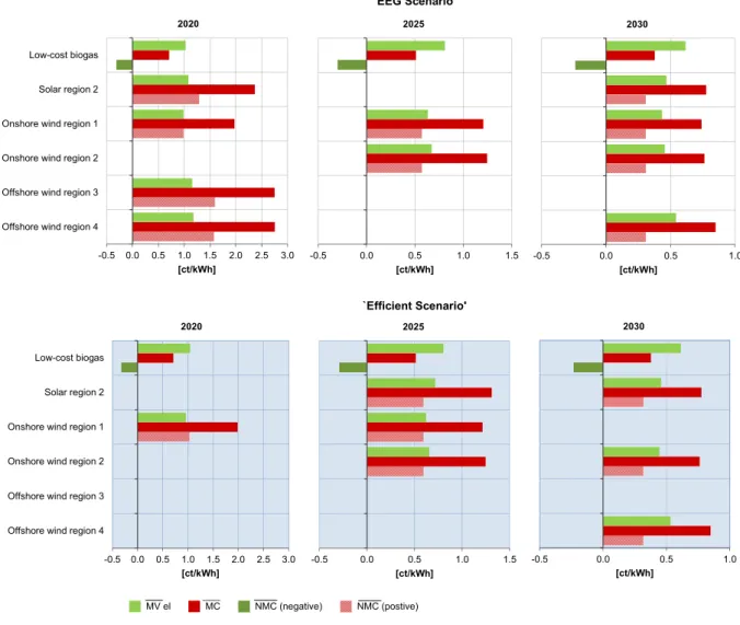
The high economic attractiveness of onshore wind power in comparison to solar power and offshore wind power up to 2020 also becomes evident when comparing the net marginal costs per kWh (N M C). Figure 4 illustrates theN M C of all renewable energy capacities built in 2020, 2025 and 2030 in the ‘EEG Scenario’ and the ‘Efficient Scenario’. We note that the scenarios differ only with regard to the RES-E targets for 2020, which are either technology- and region-specific (‘EEG Scenario’) or technology- and region-neutral (‘Efficient Scenario’). For the years 2025 and 2030, however, both scenarios assume the same technology-and region-neutral RES-E target of 40 % technology-and 48 % respectively (see Table 5).

In the ‘EEG Scenario’, N M C are not equalized across RES-E technologies and regions in 2020, which implies that the cost-efficient renewable energy mix is not achieved. As can be seen, all technologies differ with regard to both theirM C – which depend on the technology’s capital costs and full load hours – and theirM Vel _{– which depends on the unit’s revenue from selling electricity at the wholesale market. As such,} theM Vel _{is driven by the unit’s electricity generation profile or, more specifically, by the correlation between}

(21)

the unit’s hourly production factor profile and the wholesale price profile (i.e., the unit’s ‘price matching’ or ‘residual-load matching’ capability), see also J¨agemann (2014).

`Efficient Scenario' `EEG Scenario'

-0.5 0.0 0.5 1.0 1.5 2.0 2.5 3.0 Offshore wind region 4

Offshore wind region 3 Onshore wind region 2 Onshore wind region 1 Solar region 2 Low-cost biogas [ct/kWh] 2020 -0.5 0.0 0.5 1.0 1.5 [ct/kWh] 2025 -0.5 0.0 0.5 1.0 [ct/kWh] 2030 MV el MC NMC (negative) NMC (postive) -0.5 0.0 0.5 1.0 1.5 2.0 2.5 3.0

Offshore wind region 4 Offshore wind region 3 Onshore wind region 2 Onshore wind region 1 Solar region 2 Low-cost biogas [ct/kWh] 2020 -0.5 0.0 0.5 1.0 1.5 [ct/kWh] 2025 -0.5 0.0 0.5 1.0 [ct/kWh] 2030

Figure 4: M C,M Vel_and_{N M C}_{of RES-E technologies built in 2020, 2025 and 2030 (discounted with 5 %)}

Offshore wind power (in the North Sea (region 3) and Baltic Sea (region 4)) exhibits by far the high-est M C (2.75 ect2010/kWh), followed by solar power (2.37 ect2010/kWh in southern Germany (region 2)), onshore wind power (1.97 ect2010/kWh in northern Germany (region 1)) and low-cost biogas power plants (0.71ect2010/kWh). However, offshore wind power is also characterized by the highestM Vel (1.15 ect2010/kWh in the North Sea and 1.18ect2010/kWh in the Baltic Sea), followed by solar power in south-ern Germany and onshore wind power in northsouth-ern Germany (1.08 ect2010/kWh and 0.98 ect2010/kWh, respectively). Dispatchable (low-cost) biogas power plants exhibit a M Vel _{of 1.03}e_{ct2010/kWh. Overall,} it can be seen that the difference in theM C between technologies (and regions) is more pronounced than

(22)

the difference in the M Vel _{between technologies (and regions) in 2020. This effect, however, diminishes} over time since wind and solar power capacities are assumed to realize investment cost reductions, which are relatively higher for the less mature technologies (solar power and offshore wind power) than for onshore wind power which is a comparatively mature technology (see also Table A.12 of the Appendix).25

In sum, offshore wind power capacities (built to achieve commitment with the offshore wind power target by 2020) are associated with the highest N M C (1.60 ect2010/kWh in the North Sea and 1.57 ect2010/kWh in the Baltic Sea), which arises from the comparatively high capital costs of offshore wind turbines which include the costs of the onshore grid connection (see Table A.12 of the Appendix). Solar power capacities (built in order to achieve the solar power target by 2020) exhibit the second highestN M C (1.28ect2010/kWh in southern Germany), followed by onshore wind power (0.99ect2010/kWh in northern Germany). Hence, the N M C of onshore wind power capacties (built to achieve commitment with the onshore wind power target for northern Germany by 2020) are 38 % lower than theN M C of offshore wind power units and 23 % lower than the N M C of solar power units. Interestingly, these differences in the N M C in the ‘EEG Scenario’ by 2020 are primarily driven by a comparatively wide divergence of theM C between the technologies (rather than by a wide divergence of theM Vel_).

In contrast to wind and solar power technologies, which face no space potential constraints in the model, biomass (low-cost biogas and biosolid) generation is restricted by a fuel potential constraint. As a consequence, low-cost biogas generators are able to earn (windfall) profits (i.e., negative N M C of -0.32 ect2010/kWh). As explained in Section 3.1.4, space potential constraints for wind and solar power are explicitly disregarded in the model in order to prevent distortions of the economic calculus. However, if we would have accounted for space potential constraints, also wind and solar power generators would be able to earn (windfall) profits in those regions where the space potential constraint is binding. As such, binding space potential constraints for wind and solar power would prevent an equalization ofN M C across technologies and regions. More specifically, those technologies which are characterized by binding space potential constraints would be able to earn windfall profts, i.e., theirM Vel _{would exceed their}_{M C}_.

In the ‘Efficient Scenario’, commitment with the technology- and region-neutral RES-E target for 2020 is achieved with onshore wind power capacity expansions in northern Germany. TheN M C amount to 1.03 ect2010/kWh. The difference in theN M C of onshore wind power in northern Germany between the ‘EEG Scenario’ (0.99 ect2010/kWh) and the ‘Efficient Scenario’ (1.03ect2010/kWh) by 2020 is due to the fact that the onshore wind power penetration in northern Germany is higher in the ‘Efficient Scenario’ (74 GW

25_{Between 2020 and 2050, solar power and offshore wind power investment costs are assumed to decrease by 31 % and 38 %,}

(23)

or 113 TWh) than in the ‘EEG Scenario’ (50 GW or 76 TWh), which implies that theM Vel _{of an additional} onshore wind power unit in northern Germany is lower in the ‘Efficient Scenario’ than in the ‘EEG Scenario’. This result reflects the finding of the numerical ‘ceteris paribus’ example of J¨agemann (2014), i.e., theM Vel and thus also theM Vel _{of wind power decrease as penetration increases.}

As can be seen in comparing the development ofM Vel _{over time in Figure 4, the}_{M V}el _{of wind and solar} power capacities decreases as penetration increases. This is also in line with the results of the numerical ‘ceteris paribus’ example of J¨agemann (2014). However, there are several differences between the numerical ‘ceteris paribus’ example of J¨agemann (2014) and this scenario analysis, which are shortly described. First, in contrast to the numerical ‘ceteris paribus’ example which uses the revenue from selling electricity on the wholesale market within one year (8760 hours) as a proxy for the M Vel _{of wind and solar power} units, theM Vel _{derived using the electricity system optimization model corresponds to the accumulated} and discounted revenue per kWh from selling electricity on the wholesale market during all hours and years of the unit’s technical lifetime (20 years). Second, the M Vel _{determined with the electricity system} optimization model accounts for an optimal adaptation of the electricity system over time as wind and solar power penetration increases. Third, the scenario analysis examined with the electricity system optimization model also accounts for endogenous curtailment of wind and solar power generation, which also differentiates our scenario analysis from that of Lamont (2008).

As illustrated in Table 7, the actual full load hours (FLH) vary across the years in both scenarios.26 In contrast to the potential FLH shown in Table 1, the actual FLH account for wind and solar power curtailment.

Interestingly, while onshore wind power investments up to 2020 are only located in northern Germany (region 1), onshore wind turbines built from 2020 onwards are primarily deployed in southern Germany (region 2), although southern Germany (region 2) is associated with lower (potential) full load hours (FLH) and thus higherM C.27 This illustrates the benefit of regional diversification. The significant expansion of onshore wind power in northern Germany in 2020 causes the M Vel _{of an additional onshore wind power} unit in northern Germany to decrease.28 As a consequence, the comparative cost advantage of onshore wind power in northern Germany over onshore wind power in southern Germany – which was originally driven by higher potential FLH and thus lower M C – diminishes. In fact, at some penetration level of onshore wind power in northern Germany, onshore wind power in southern Germany begins to have a comparative

26_{The amount of wind and solar power curtailment in GWh is shown in Table A.17 of the Appendix.} 27_{See Table 1 and Figure 3.}

(24)

Table 7: Actual annual full load hours of wind and solar power plants [h]

2020 2025 2030 2035 2040 2045 2050

‘EEG Scenario’

Onshore wind power region 1 1,528 1,510 1,484 1,478 1,479 1,519 1,491

Offshore wind power region 3 3,420 3,418 3,409 3,249 3,268 3,420

Offshore wind power region 4 3,349 3,349 3,344 3,345 3,342 3,349 3,348

Solar power region 1 992 991 990 962 964

Solar power region 2 1,084 1,084 1,084 1,084 1,084 1,084 1,084

‘Efficient Scenario’

Offshore wind power region 3 3,418 3,338 3,243 3,149 3,420

Offshore wind power region 4 3,349 3,234 3,344 3,341 3,343 3,349 3,347

Solar power region 1 992 988 980 943 957

Solar power region 2 1,084 1,084 1,084 1,084 1,084 1,084 1,084

cost advantage over onshore wind power in northern Germany. Hence, investments in onshore wind power turbines in southern Germany become efficient, although southern Germany exhibits lower potential FLH and thus higher M C than onshore wind power turbines in northern Germany.29 _{This is due to the fact} that the production factor profile of onshore wind turbines in southern Germany is characterized by a higher price-matching (or residual-load matching) capability than the production factor profile of onshore wind turbines in northern Germany – given the comparatively large penetration of onshore wind power in northern Germany and the associated short-term merit-order effect. As a consequence, theM Vel_{of onshore} wind turbines in southern Germany exceeds theM Vel_{of onshore wind turbines in northern Germany, which} compensates for the higher M C in southern Germany. A second factor which deteriorates the economic attractiveness of additional onshore wind power capacities in northern Germany (as penetration increases) is the increasing curtailment of onshore wind power in northern Germany, which reduces the actual FLH (see Table 7). As a consequence, the difference in the (actual) FLH between onshore wind power in northern and southern Germany diminishes. Moreover, theM C of onshore wind power in northern Germany increases.

In addition to onshore wind power, solar power is also expanded in southern Germany (region 2) under the technology- and region-neutral RES-E target by 2025 despite comparatively highM C (see Figure 3). This reflects the benefit of technological diversification in reaching politically implemented RES-E targets. Overall, onshore wind and solar power capacity expansions in 2025 take place up to the point at which the

29_{The potential FLH of onshore wind power plants in southern Germany are assumed to be more than 5 % lower than the}

(25)

N M C are equalized (see Figure 4), which is in line with the economic theory discussed in Section 2. The same holds true for the year 2030, in which theN M C are equalized across solar power, onshore wind power and offshore wind power units.

As a consequence of the technology- and region-specific RES-E targets for 2020 – which prevent the equalization of theN M C across renewable energy technologies and regions (see Figure 4) – excess costs of 6.6 Bne2010 occur. These are defined by the difference in accumulated discounted system costs between the ‘EEG Scenario’ and the ‘Efficient Scenario’.

The comparison of N M C between technologies and regions in 2020 shows that excess costs are driven by the technology-specific offshore wind and solar power targets for 2020 (of 22 and 56 TWh, respectively). Although the onshore wind power penetration is much higher in 2020 than the offshore wind and solar power penetration in the ‘EEG Scenario’ (in terms of TWh),N M C of onshore wind power is significantly lower than theN M C of offshore wind and solar power (see Figure 4). This illustrates the low economic attractiveness of offshore wind and solar power in comparison to onshore wind power up to 2020.

Figure 5 shows the interdependence between the wind and solar power penetration (i.e., the annual wind and solar power generation) and the annual correlation (between the wind and solar power generation profile and the wholesale price profile) for both scenarios. Overall, the annual correlation tends to decrease as the annual wind and solar power generation increases, which is in line with the results derived in J¨agemann (2014). This can, for example, be seen in the ‘Efficient Scenario’: Between 2015 and 2020, onshore wind power in northern Germany (region 1) is significantly expanded, which leads to a drop in the correlation (between the onshore wind power production factor profile in northern Germany (region 1) and the wholesale price profile). The same effect can be observed for solar power in southern Germany (region 2) between 2020 and 2025.

However, Figure 5 also illustrates the importance of cross-technological effects. For example, between 2020 and 2025, the correlation of onshore wind power in northern Germany (region 1) increases, although the penetration of onshore wind power in northern Germany slightly increases (from 74 GW in 2020 to 85 GW in 2025). This is due to the significant increase in solar power generation in southern Germany (region 2) which is negatively correlated with the onshore wind production factor profile in northern Germany (region 1). This is shown in Table 8.

(26)

-1.0 -0.8 -0.6 -0.4 -0.2 0.0 0.2 0 50 100 150 200 250 300 350 400 450 500 2015 2020 2025 2030 C o rr el at io n G en er at io n [T W h ] 'Efficient Scenario' -1.0 -0.8 -0.6 -0.4 -0.2 0.0 0.2 0 50 100 150 200 250 300 350 400 450 500 2015 2020 2025 2030 C o rr el at io n G en er at io n [T W h ] `EEG Scenario' Solar region 1 Solar region 2

Onshore wind region 1

Offshore wind region 3

Solar region 1

Solar region 2

Figure 5: Annual generation [TWh] and annual correlation between the wind/solar power generation profile and the wholesale price profile

Although the correlation between the onshore wind generation profile in northern Germany (region 1) and the wholesale price profile increases between the years 2020 and 2025, this does not mean that the onshore wind power units that were built in 2020 in northern Germany (region 1) are more profitable in 2025 than in 2020 – profitable in the sense that the revenue per MW from selling electricity on the wholesale market in 2025 exceeds the revenue in 2020. In contrast, the additional onshore wind and solar power in southern Germany (region 2) has a downward effect on the wholesale price in 2025, which lowers the annual revenue of onshore wind power turbines in northern Germany (region 1) that were built in 2020 (see Figure 6).

(27)

0 20 40 60 80 100 2020 2025 2030 2035 2040 T h o u sa n d € /M W

Onshore wind reg 1

Figure 6: Development of the annual revenue from selling electricity on the wholesale market of an onshore wind power turbine built in region 1 in 2020 in the ‘Efficient Scenario’ [thousande/MW] (not discounted)

Overall, the revenue earned from selling electricity on the wholesale market significantly varies across the years. The comparatively low revenue of onshore wind power turbines in northern Germany (region 1) in 2035 is due to the offshore wind power expansion in the Baltic Sea (region 4) by 2035, which exhibits a high positive correlation with onshore wind power in northern Germany of 0.5 (see Table 8). However, the increase in the revenue of onshore wind power in northern Germany by 2040 can be explained by a decrease in the onshore wind power penetration in northern and southern Germany. Betwen 2035 and 2040, more than 13 GW of onshore wind power capacities are decommissioned (9 GW in northern Germany and 4 GW in southern Germany), which are not replaced. Moreover, electricity generation from flexible gas-fired power plants increases. The increase in the annual revenue of wind and solar power plants in the longer run can also be seen in Figures A.8 and A.9 of the Appendix, which show the annual revenue of onshore wind, offshore wind and solar power plants that were built in 2025 and 2030. Hence, the optimal adaptation of the dispatchable power plant mix to a system with a higher share of flexible gas-fired (peak-load) power plants and a lower share of lignite-fired (base-load) power plants in Germany (see Figure A.7 of the Appendix) benefits wind and solar power generators in the long-run.

(28)

Table 8: Correlations between production factor profiles of wind and solar power technologies

Solar Solar Onshore wind Onshore wind Offshore wind region 1 region 2 region 1 region 2 region 3 Solar 0.8 region 2 Onshore wind -0.2 -0.1 region 1 Onshore wind -0.2 -0.2 0.5 region 2 Offshore wind -0.3 -0.2 0.6 0.4 region 3 Offshore wind -0.2 -0.2 0.5 0.4 0.6 region 4

In summary, the presented scenario results derived with the electricity system optimization model confirm the theoretical results derived in J¨agemann (2014) and Section 2 and illustrate the economic inefficiency associated with Germany’s technology- and region-specific RES-E targets for 2020. Due to the significantly higherN M C of offshore wind and solar power units compared to onshore wind power units in Germany up to 2020, the technology- and region-specific RES-E targets are associated with excess costs of more than 6.6 Bne2010 (accumulated and discounted).

However, the quantified excess costs of 6.6 Bne2010should be interpreted as a lower bound estimate for the overall inefficiency associated with Germany’s technology- and region-specific RES-E targets for 2020. This is due to the fact that power transfers between the regions within Germany, i.e., from northern to southern Germany and vice versa, face no transmission constraints.

More specifically, while power exchange between Germany and neighboring countries is limited by ex-ogenously defined interconnection capacities, a copper-plate with no congestions is assumed for Germany. However, as soon as transmission capacity bottlenecks between two regions occur, the value of power supply (at a specific point in time) differs between the regions. As such, the marginal value (M Vel) of wind and solar power capacities between two regions may not only vary because of differences in the production factor profiles but also due to transmission capacity bottlenecks. The applied model, however, fails to account for the latter effect.

As such, the large expansion of onshore wind power in northern Germany up to 2020 (realized under the technology- and region-neutral RES-E target in the ‘Efficient Scenario’) may not be optimal (i.e., too large) when accounting for transmission capacity bottlenecks from northern to southern Germany, which already exist today and which are expected to increase as wind power supply in northern Germany rises. More

(29)

specifically, onshore wind capacities are expected to become efficient in southern Germany already by 2020 when accounting for transmission capacity bottlenecks from northern to southern Germany, substituting part of the investments in northern Germany. Hence, we argue that the economic inefficiency associated with the region-specific onshore wind power target for northern Germany is underestimated with our model, which implies that the overall excess costs of 6.6 Bne2010 (accumulated and discounted) represent a lower bound estimate.

Moreover, the model is deterministic and not stochastic in its nature. Hence, no uncertainty about the hourly or yearly electricity generation of wind and solar technologies is incorporated. In stochastic models, the uncertainty of wind and solar power generation can be modeled by weighting different scenarios (which vary with regard to the wind and solar power production factor profiles) by their specific probability of occurence (Nagl et al. (2013)). As a means to reduce risk, the renewable energy mix determined by a stochastic model is expected to be more divers (both with regard to technologies and regions) than the renewable energy mix determined by a deterministic model (given a technology- and region-neutral RES-E target). However, unlike the impact of disregarding transmission capacity bottlenecks on the level of excess costs, the consequences of abstracting from uncertainty is not straight forward. Hence, it cannot be said a priori in which direction the excess costs of technology- and region-specific RES-E targets would change (in comparison to the present analysis) if a stochastic rather than a deterministic model would have been applied.

4. Conclusion

It has been shown that comparing the economic attractiveness of renewable energy technologies on the basis of marginal costs per kWh (M C) is incorrect, as doing so neglects the marginal value per kWh (M Vel₎ of the respective technology. Instead, thenet marginal costs per kWh (N M C) should serve as the reference when discussing the economic attractiveness of renewable energy technologies. Renewable energy support schemes that fail to incentivize investors to account for differences in theM Vel _{prevent an equalization of} N M C across technologies and regions in the equilibrium and thus are associated with excess costs. For the case of Germany and its technology- and region-specific wind and solar power targets for 2020, excess costs amount to more than 6.6 Bne2010 (accumulated and discounted). These are driven by the comparatively highN M C of offshore wind and solar power in comparison to onshore wind power in Germany up to 2020. However, given the fact that we abstract from transmission capacity bottlenecks within Germany in the model, the quantified excess costs should be interpreted as a lower bound estimate.

(30)

Future research could address the following issues: First, the model could be extended to acount for both transmission capacity limitations within Germany and stochastic wind and solar power generation. Second, the technical granularity of wind and solar power systems could be increased to account for differences in the production factor profiles of wind and solar power units due to an alternative sizing of the wind power turbine or due to an alternative orientation of the PV system. This would allow us to analyze, for example, at which point in time (or at which penetration level) theN M C of PV systems that are tilted to the east or the west have lower N M C than PV systems that are tilted to the south. Third, an alternative model could be applied which maximizes investor’s profits rather than minimizing total system costs. Fourth, as pointed out by Mitchell et al. (2006) and Klessmann et al. (2008), there is some trade-off associated with exposing renewable energy investors to market risk as it increases the project’s capital costs, which may, in turn, deteriorate the (dynamic) efficiency of the support scheme. This is an important aspect if the goal is to bring new technologies into the market and gain experience. Meanwhile, however, renewables account for a comparatively large share of total electricity supply in many countries (e.g., 25 % in Germany in 2013 (Statista (2014))). Hence, efficiency gains due to the consideration of the market price signal in the generator’s investment decisions are likely to balance potential efficiency losses due to higher risk premiums and higher required support payments. This could also be an interesting opportunity for further research.

(31)

References

Agora Energiewende, 2013. Studie zum kostenoptimalen Ausbau der Erneuerbaren Energien. Hintergrunddokument zu Koste-nannahmen der Erneuerbaren. Tech. rep.

BMU, 2014. Eckpunkte f¨ur die Reform des EEG. Tech. rep., Federal Ministry for the Environment, Nature Conservation, Building and Nuclear Safety.

CDU/CSU/SPD, 2013. Deutschlands Zukunft gestalten. Koalitionsvertrag zwischen CDU, CSU und SPD. 18. Legislaturperiode. Tech. rep.

URLhttps://www.cdu.de/sites/default/files/media/dokumente/koalitionsvertrag.pdf

Deutsche Bank, 2012. The German Feed-in Tariff: Recent Policy Changes. Tech. rep., Deutsche Bank. URLhttps://www.db.com/cr/en/docs/German_FIT_Update_2012.pdf

ENSTO-E, 2013. Hourly load values for all countries for a specific month. URLhttps://www.entsoe.eu/data/data-portal/consumption/

ENTSO-E, 2012. 10-Year Network Development Plan.

ENTSO-E, February 2014. Monthly consumption of all countries for a specific year (2012).

URLhttps://www.entsoe.eu/db-query/consumption/monthly-consumption-of-all-countries-for-a-specific-year/

EU Council, October 2009. Brussels European Council 29/30 OCTOBER 2009 - Presidency Conclusions. Council of the European Union.

EuroWind, 2011. Database for hourly wind speeds and solar radiation from 2006-2010 (not public).

EWI, 2010. European RES-E policy analysis - a model based analysis of RES-E deployment and its impact on the conventional power markt. M. F¨ursch and C. Golling and M. Nicolosi and R. Wissen and D. Lindenberger (Institute of Energy Economics at the University of Cologne).

EWI, 2011. Roadmap 2050 - a closer look. Cost-efficient RES-E penetration and the role of grid extensions. M. Fürsch, S. Hagspiel, C. Jägemann, S. Nagl and D. Lindenberger. Institute of Energy Economics at the University of Cologne. Frontier Economics, 2012. Die Zukunft des EEG - Handlungsoptionen und Reformansätze. Bericht für die ENBW Energie

Baden-W¨urtemberg AG. Tech. rep., Frontier Economics.

Fürsch, M., Hagspiel, S., Jägemann, C., Nagl, S., Lindenberger, D., Tröster, E., 2013. The role of grid extensions in a cost-efficient transformation of the European electricity system until 2050. Applied Energy 104, 642–652.

IEA, 2010a. Technology roadmap - concentrating solar power. International Energy Agency. URLwww.iea.org/papers/2010/

IEA, 2010b. World Energy Outlook 2010. International Energy Agency. IEA, 2011. World Energy Outlook 2011. International Energy Agency.

ISE, 2013. Stromgestehungskosten für Erneuerbare Energien. Tech. rep., Fraunhofer-Institut für solare Energiesysteme. ISE, 2014. Stromerzeugung aus Solar- und Windenergie im Jahr 2013. Tech. rep., Fraunhofer-Institut für solare Energiesysteme

ISE.

J¨agemann, C., 2014. An illustrative note on the system price effect of wind and solar power - The German case. Institute of Energy Economics at the University of Cologne Working Paper No 14/10.

J¨agemann, C., F¨ursch, M., Hagspiel, S., Nagl, S., 2013a. Decarbonizing Europe’s power sector by 2050 - Analyzing the economic implications of alternative decarbonization pathways. Energy Economics 40, 622 – 636.

J¨agemann, C., Hagspiel, S., Lindenberger, D., 2013b. The economic inefficiency of grid parity: The case of German photovoltaic. Institute of Energy Economics at the University of Cologne Working Paper No 13/19.

Joskow, P. L., 2011. Comparing the costs of intermittent and dispatchable electricity generating technologies. American Eco-nomic Review 100(3), 238–241.

Klessmann, C., Nabe, C., Burges, K., 2008. Pros and cons of exposing renewables to electricity market risks - A comparison of the market integration approaches in Germany, Spain, and the UK. Energy Policy 36, 3646 – 3661.

Lamont, A. D., 2008. Assessing the long-term system value of intermittent electric generation technologies. Energy Economics 30, 1208 – 1231.

Mitchell, C., Bauknecht, D., Connor, P. M., 2006. Effectiveness through risk reduction: a comparison of the renewable obligation in England and Wales and the feed-in system in Germany. Energy Policy 34, 297 – 305.

Nagl, S., Fürsch, M., Jägemann, C., Bettzüge, M., 2011. The economic value of storage in renewable power systems - the case of thermal energy storage in concentrating solar plants. Institute of Energy Economics at the University of Cologne Working Paper No 11/08.

Nagl, S., F¨ursch, M., Lindenberger, D., 2013. The costs of electricity systems with a high share of fluctuating renewables - a stochastic investment and dispatch optimization model for Europe. The Energy Journal 34, 151–179.

PROGNOS/EWI/GWS, 2010. Energieszenarien für ein Energiekonzept der Bundesregierung. Schlesinger and P.Hofer and A. Kemmler and A. Kirchner and S. Strassburg (all Prognos AG); D. Lindenberger and M. Fürsch and S. Nagl and M. Paulus and J. Richter and J. Trüby (all Institute of Energy Economics at the University of Cologne); C. Lutz and O. Khorushun and U. Lehr and I. Thobe (all GWS mbH).

Richter, J., 2011. DIMENSION - A Dispatch and Investment Model for European Electricity Markets (Working Paper No. 11/03) Institute of Energy Economics at the University of Cologne.

URLhttp://www.ewi.uni-koeln.de/publikationen/working-paper/

Statista, January 2014. Anteil erneuerbarer Energien an der Bruttostromerzeugung in Deutschland in den Jahren 1990 bis 2013. http://de.statista.com/statistik/daten/studie/1807/umfrage/erneuerbare-energien-anteil-der-energiebereitstellung-seit-1991/.